Additional file 1: A transposable elements annotation pipeline and expression analysis reveal potentially active elements in the microalga Tisochrysis lutea Jérémy Berthelier1*, Nathalie Casse2, Nicolas Daccord3, Véronique Jamilloux4, Bruno Saint-Jean1, Grégory Carrier1 1: IFREMER, Physiology and Biotechnology of Algae Laboratory, rue de l’Ile d’Yeu, 44311 Nantes, France. 2: Mer Molécules Santé, EA 2160 IUML, FR 3473 CNRS, Le Mans University, Le Mans, France 3: Institut de Recherche en Horticulture et Semences, INRA of Angers, France 4: Research Unit in Genomics-Info, INRA of Versailles, Versaille, France
*
Corresponding author:
[email protected]
Table of Contents Table S1: Bibliography of tools related to TE detection. ......................................................................... 2 Figure S1: Illustration of the “Russian doll” strategy .............................................................................. 3 Figure S2: Comparison of the detection step of PiRATE ........................................................................ 4 Figure S3: Evaluation of the classification step of PiRATE....................................................................... 5 Figure S4: Genome composition of Tisochrysis lutea.............................................................................. 5 Method S1: Annotation of the potential autonomous TEs ..................................................................... 6 Table S2: Rules established to annotate potentially autonomous TEs ................................................... 6 Method S2: Annotation of TEs and repeated elements in the genome of Tisochrysis lutea. ................. 7 Table S3: Rules established to annotate the TE content in the Tisochrysis lutea genome ..................... 7 Method S3: Contribution of each TE detection approach, depending on the input data. ..................... 8
Table S1: Bibliography of tools related to TE detection. The “*” indicates the 12 tools used in the detection step of PiRATE. Name
Website
Author(s)
Similarity-based tools RepeatMasker*
www.repeatmasker.org/
Censor
http://www.girinst.org/censor/download.php
Smit and Hubley, 1997 Kohany et al., 2006
Windowmasker
ftp.ncbi.nlm.nih.gov/pub/agarwala/windowmasker
Morgulis et al., 2006
Transposon-PSI
transposonpsi.sourceforge.net/
Haas, 2007
TeClass
http://www.compgen.uni-muenster.de/teclass/index.hbi?
Abrusan et al., 2009
RepClass
https://sourceforge.net/projects/repclass/
Feschotte et al.,2009
TARGeT
http://target.iplantcollaborative.org
Han et al., 2009
TESeeker
http://repository.library.nd.edu/view/27/teseeker
Kennedy et al., 2011
PASTEClassifier
https://urgi.versailles.inra.fr/Tools/PASTEClassifier
Hoede et al., 2014
TE-HMMER*
http://www.seanoe.org/data/00406/51795/
Berthelier et al., 2017
Structural-based tools TRANSPO
http://alggen.lsi.upc.es/recerca/search/transpo/transpo.html
Santiago et al., 2002
TSDfinder
http://www.ncbi.nlm.nih.gov/CBBresearch/Landsman/TSDfinder/
LTR_STRUC
http://www.mcdonaldlab.biology.gatech.edu/ltr_struc.htm
MAK
http://nar.oxfordjournals.org/content/31/13/3659.long
Szak et al., 2002 McCarthy and McDonald, 2003 Yang and Hall, 2003
LTR_MINER
http://genomebiology.com/content/supplementary/gb-2004-5-10-r79-s5.pl
LTR_par
http://www.eecs.wsu.edu/~ananth/software.htm
LTR_FINDER
http://tlife.fudan.edu.cn/ltr_finder/
LTRharvest*
http://www.zbh.uni-hamburg.de/?id=206
LTRdigest
http://www.zbh.uni-hamburg.de/?id=207
MUST
http://www.healthinformaticslab.org/supp/
HelSearch*
http://omictools.com/helsearch-tool
MGEScan-LTR MGEScannonLTR*
http://darwin.informatics.indiana.edu/cgi-bin/evolution/daphnia_ltr.pl
Chen et al., 2009 Lixing and Bennetzen, 2009 H. Tang, 2009
http://darwin.informatics.indiana.edu/cgi-bin/evolution/nonltr/nonltr.pl
H. Tang, 2009
Pereira, 2004 Kalyanaraman and Aluru, 2006 Xu and Wang, 2007 Ellinghaus et al., 2008 Steinbiss et al., 2009
MITE-Hunter*
http://target.iplantcollaborative.org/mite_hunter.html
Sine-Finder*
http://www.jstor.org/stable/41434686?seq=1#page_scan_tab_contents
Han and Wessler, 2010 Wenke et al., 2011
RSPB
http://pmite.hzau.edu.cn/MITE/tools/
Lu et al., 2012
MITE-Digger
http://omictools.com/mite-digger-tool
Yang, 2013
TIRfinder
https://sourceforge.net/projects/tirfinder/
Gambin et al., 2013
HelitronScanner
http://omictools.com/helitronscanner-tool
Xiong et al., 2014
detectMite
https://sourceforge.net/projects/detectmite/
SINE_scan
https://github.com/maohlzj/SINE_Scan
MUSTv2
http://www.healthinformaticslab.org/supp/resources.php
congtig et al., 2016 Mao and Wang, 2016 Ge et al., 2017
Repetitiveness-based tools REPuter
https://bibiserv2.cebitec.uni-bielefeld.de/reputer
RepeatFinder
http://cbcb.umd.edu/software/RepeatFinder/
Kurtz and Schleiermacher, 1999 Volfovsky et al., 2001
RECON
http://selab.janelia.org/recon.html
RepeatScout*
http://www.repeatscout.bioprojects.org/
Bao and Eddy, 2002 Quesneville et al., 2003 Edgar and Myers, 2005 Price et al., 2005
GROUPER
https://urgi.versailles.inra.fr/Tools/REPET
PILER
http://www.drive5.com/piler/
Repseek
http://wwwabi.snv.jussieu.fr/public/RepSeek/
Achaz et al., 2006
Pclouds
http://www.evolutionarygenomics.com/ProgramsData/PClouds/PClouds.html
Gu et al., 2008
Tallymer
http://www.zbh.uni-hamburg.de/?id=211
Kurtz et al., 2009
TEdenovo*
http://urgi.versailles.inra.fr/Tools/REPET
RepeatModeler
http://www.repeatmasker.org/RepeatModeler.html
Flutre et al., 2011 Smit and Hubley, 2014
Build repeated elements ReAS
ftp://ftp.genomics.org.cn/pub/ReAS/software/
Li et al., 2005
RepeatExplorer*
http://galaxy.umbr.cas.cz:8080/
Novák et al., 2013
RepARK*
https://github.com/PhKoch/RepARK
Koch et al., 2014
Tedna
https://urgi.versailles.inra.fr/Tools/Tedna
Zytnicki, 2014
dnaPipeTE*
https://lbbe.univ-lyon1.fr/-dnaPipeTE-
Transposome
https://github.com/sestaton/Transposome
Goubert et al., 2015 Staton and Burke, 2015
REPdenovo
https://github.com/Reedwarbler/REPdenovo
Chu et al., 2016
Figure S1: Illustration of the “Russian doll” strategy employed for the implementation of the libraries used to annotate the potentially autonomous TEs, total TE content and repeated element content of Tisochrysis lutea.
100%
% of TE families with PiRATE % of TE families with TEdenovo 91% 88%
80%
84% 84% 79%
73% 73% 71% 67%
60% 40% 20% 0%
35% 33%
32% 23% 18%
20% 20%
% of TE families with PiRATE % of TE families with TEdenovo
b Percentage of TE families
Percentage of TE families
a
100% 80%
96%
94% 94% 92% 81% 80% 81% 75%
79% 62%
60% 40%
47%
60% 60% 52%
27% 27%
20% 0%
Figure S2: Comparison of the detection step of PiRATE and TEdenovo by calculating the percentage of detected TE families for each TE order of Arabidopsis thaliana with: a) a complete length (coverage score ≥ 70%), b) a complete and a partial length (coverage score ≥ 40%). The x-axis indicates the number of TE families for each order; “n-a” means nonautonomous.
100%
98% 87%
Percentage of TE families
100%
91%
80%
72%
60%
54%
50%
40%
33%
20%
27% 21%
19%
17%
13%
7%
7% 1% 1%
2%
0%
0% 0%
0%
LTR (148) LINE (15) SINE (6)
Classification :
TIR (43)
Correct
n-a TIR (48)
Incorect
Helitron (3)
n-a Helitron (29)
noCAT
Figure S3: Evaluation of the classification step of PiRATE. Percentage of detected families that were correctly classified, incorrectly classified or classified as uncategorized for each TE order of Arabidopsis thaliana. The classification step of PiRATE was able to correctly classify 75% of the detected TE families in A. thaliania. The x-axis indicates the number of TE families for each order; “n-a” means non-autonomous.
Transposable elements
20.84
Uncategorized repeated…
17.79
Simple repeats
5.97
Protein-coding genes
38.49
Non-characterized
16.91
0
10
20
30
40
Proportion of the genome (%)
50
Figure S4: Genome composition of Tisochrysis lutea. Proportion of the protein-coding genes, transposable elements, simple repeats, uncategorized repeated elements and uncharacterized sequences.
Method S1: Annotation of the potential autonomous TEs in the genome of Tisochrysis lutea. Using the annotation file obtained with TEannot from the “potential autonomous TEs” library, we established several rules to select potential autonomous TEs depending on the superfamily. First, we established a minimum length depending on the TE order. For example, a minimum length of 4000 bp for the annotated LTR/Copia elements. We also established a “length threshold” value by dividing the “reference TE length” by the “annotate TE length”. If this threshold value is 1, a given annotate sequence and its referent sequence have the same length. We choose a minimum and a maximum “length threshold” value for each TE order. We selected the annotated sequences with the highest and lowest threshold value and checked for the presence of conserved domain(s) with Pfam or Blastx. If no domain(s) were found, the value of the threshold was decreased or increased respectively until annotated sequences bearing conserved domain(s) were detected. In addition, we established a minimum percentage of identity for the TIR elements. With a manual check, the most suitable value was 90%. The overview of the applied rules is described in Table S2. Annotated sequences had to meet the required minimum length, minimum % of identity and length thresholds in order not to be excluded. Table S2: Rules established to annotate potentially autonomous TEs in the genome of Tisochrysis lutea. Class I TEs Minimum length (bp) Minimum % of identity Minimum length threshold Maximum length threshold
Class II TEs
LTR/Copia 4000
LTR/Gypsy 4000
LINE/L1 2500
TIR/hAT 1300
TIR/Mariner 1000
TIR/PiggyBac 1000
TIR/Harbinger 1000
60 (default)
60
60
90
90
90
90
/
0.97
0.78
0.98
0.995
0.997
0.93
/
1.84
1.2
1.03
1.005
1.003
1.36
Method S2: Annotation of TEs and repeated elements in the genome of Tisochrysis lutea. From the annotations file obtained with TEannot from the “total TE library”, we also established several rules to select the potentially autonomous TEs and non-autonomous TEs. We used the same method as that used in Method S1. We established a minimum length of 200 bp to be able to annotate potential TE fossils. We established minimum and a maximum “length threshold” values of 0.5 and 1.5, respectively. We also chose a minimum percentage of identity of 90% for the TIR elements. Annotated sequences had to meet the minimum length, minimum % of identity and length thresholds in order not to be excluded. The overview of the applied rules is given in Table S3. Finally, to measure the proportion of the uncategorized repeated elements of the T. lutea genome, we used the annotations file obtained with TEannot from the “repeated elements library”. We established a minimum length of 200 bp. The proportion of every annotated repeated element in the genome of T. lutea was obtained. We subtracted this proportion from the “total TEs” proportion to obtain an estimation of the uncategorized repeats.
Table S3: Rules established to annotate the TE content in the Tisochrysis lutea genome Class I TEs Minimum length (bp) Minimum % of identity Minimum length threshold Maximum length threshold
Class II TEs
LTR/Copia 200
LTR/Gypsy 200
LINE/L1 200
TRIM 200
LARD 200
SINE 200
TIR/hAT 200
TIR/Mariner 200
TIR/PiggyBac 200
TIR/Harbinger 200
MITE 200
60
60
60
60
60
60
90
90
90
90
90
0.5
0.5
0.5
0.5
0.5
0.5
0.5
0.5
0.5
0.5
0.5
1.5
1.5
1.5
1.5
1.5
1.5
1.5
1.5
1.5
1.5
1.5
Method S3: Contribution of each TE detection approach, depending on the input data. The detection step (Fig. 1) of PiRATE was launched with raw Tisochrysis lutea Illumina data and either the previous draft version of the T. lutea genome or the new T. lutea genome. For both these cases the detected sequences were compared with PASTEC to the 240 reference sequences representing the 174 potentially autonomous TE families that we found in the T. lutea genome (Results and Discussion, 2.4.1). For both cases, we selected each detected sequence matching with a T. lutea TE family. For each detected TE family, we selected the detected sequences with the highest percentage of coverage. We normalized the percentage of coverage of the detected sequences obtained from the draft genome assembly and raw Illumina data with the percentages of coverage of the corresponding detected sequences obtained with the new genome and raw Illumina data. We counted the number of TE families that were detected from the draft genome assembly and the raw Illumina data (having a normalized percentage of coverage of at least 40%). We estimated the contribution of each TE detection approach, depending on the input data. For each detection approach, we counted the number of TE families of T. lutea detected with the largest length (highest percentage of coverage compares to reference TE sequences) and divided this number by the total of TE families detected. This provided an estimation of the contribution of each TE detection approach depending on the input data (Main manuscript Fig. 3).