processing pipeline. DTI data were corrected for Eddy current distortion and head movement with the FSL diffusion imaging toolbox 2. b0 images from the ...
Additional information on image processing and rich-club analyses
Imaging parameters and image processing MRI data were acquired with a 3T MRI scanner (Skyra, Siemens Medical Systems, Erlangen, Germany). The MRI protocol included the following sequences: 3D magnetization prepared rapid acquisition gradient-echo (MPRAGE) T1 weighted sequence (TR/TE = 1900ms/2.46ms; TI=900ms; 192 slices, voxel size 0.9×0.9×0.9 mm, no gap, matrix=256x256, FOV = 240mm), a T2 sequence (TR/TE = 2800ms/90ms; 43 slices, voxel size 0.5×0.5×3.0 mm, no gap, matrix=256x256, FOV = 240mm), a 3D fluid attenuated inversion recovery (FLAIR) sequence (TR/TE = 4700ms/392ms; TI=1800 ms; 192 slices, voxel size 0.8×0.8×0.9 mm, no gap, matrix=256x256, FOV = 240mm) and diffusion tensor imaging (DTI, single-shell, 20 directions with non-collinear diffusion gradients (b = 1000 s/mm2) and one nondiffusion-weighted (b = 0 s/mm2), voxel size 1.9×1.9×2.0 mm, FOV 240x240 mm, matrix 128 x 128, all volumes averaged over three acquisitions, TR/TE = 5500ms/83ms; 35 slices, no gap). Images were processed with the functional imaging software library (FSL, version 5.0, www.fmrib.ox.ac.uk). 3D-sequences were reoriented to standard space and field bias was corrected for T1 and T2 weighted images using the maps from FSL-FAST. T1 and FLAIR images were registered to T2-weighted images for lesion mapping. T1hypointense and T2-hyperintense lesions were outlined on T2 and registered T1 images with a seed-based semiautomatic algorithm using the software Analyze 11.0 (AnalyzeDirect, www.analyzedirect.com). Brain tissue volume, normalised for subject head size, was estimated with SIENAX 1. To avoid segmentation errors, lesion filling was performed by filling marked lesion areas on T1 images with mean intensity values from the lesions’ surrounding parenchyma. Normalized brain volumes (NBV)
as well as normalized grey matter (NGM) and white matter (NWM) volumes were extracted with a modified SIENAX script. Instead of the integrated automated brain extraction tool (BET), we ran BET separately in advance and manually corrected brain masks if needed. Individual T1- and T2-lesion volumes were normalized according to the normalization factor from SIENAX. In addition, we used Freesurfer software (Version 5.2.0) for cortical reconstruction and volumetric segmentation (http://surfer.nmr.mgh.harvard.edu/). Again, brain masks and white / grey matter segmentation errors were manually corrected in all cases. For each individual subject, the cortical surface was parcellated into 86 distinct regions (i.e, 43 cortical and subcortical grey matter regions per hemisphere). Their corresponding subcortical white matter regions were used for probabilistic tractography using the FSL processing pipeline DTI data were corrected for Eddy current distortion and head movement with the FSL diffusion imaging toolbox 2. b0 images from the DTI-sequences were registered linearly to T1 images and inverse registration matrices were used to transfer structural masks from FreeSurfer into DTI-space. Further processing of the DTI images included the fitting of a diffusion tensor model at each voxel with dtifit. To run probabailistic tractography, data were preprocessed with BEDPOSTX of FSL, which builds up distributions on diffusion parameters at each voxel and allows to model crossing fibres (including the number of crossing fibres) within each voxel of the brain 2
. We used the 86 FreeSurfer region masks as seed regions and defined no target
masks, but an exclusion mask for fractional anisotropy (FA) values below 0.15. Tracking was performed with 5000 seeds per voxel, a curvature threshold of 0.2 and a step length of 0.5. We used the same 86 FreeSurfer region masks to extract the number of streamlines reaching a region from every other of the 86 regions.
Reconstruction of brain networks Networks are mathematically defined as a graph G=(V,E) with a number of nodes or vertices (V) and connections or edges (E) between the nodes. There is an on-going debate about the best method defining connections between two brain regions i and j and how to reconstruct representative and reliable networks 3–5. Here, FreeSurfer regions were taken as vertices and the number of streamlines between two nodes i and j as connection. Based on these data, two kinds of networks G or their corresponding connectivity matrices M were defined. First, binary networks (0=unconnected, 1=connected) were constructed (Gbin). A connection between i and j was labelled as present if any stream from the seed region entered the target region. This approach disregards the strength of connections between regions and might lead to a completely connected network. To avoid completely connected networks, connections below a certain threshold (e.g. 80% of maximum raw connection strength) were excluded. Currently, there is no consensus about the optimal cut-off for such thresholds 6. We, therefore, investigated the effect of thresholds from 2.5% to 97.5% in steps of 2.5% in patients and healthy controls to identify a meaningful cut-off. We arbitrarily used the small world index (SWI) as global read out for thresholding. The small-world measure combines clustering and average path length (APL) compared to random networks.7 Small world features of a network may be assumed if clustering is high and APL low. Networks with a SWI above one are generally considered to have small world properties, while a range between one and three is sometimes seen as borderline value 7. The small-world measure is considered to be a rather unspecific but robust network feature. We hypothesized that an increase of the variance of the small-world measure might therefore indicate a major bias through thresholding of raw networks. At each threshold we defined Gbin and constructed 100 random networks (Grand) with
the same degree distribution to calculated SWI = clustering(Gbin)/clustering(Grand) / APL(Gbin)/APL(Grand). We aimed to define the best cut-off for further analyse based on these results. In contrast to binary networks, weighted networks hold as well information about the connection strength between two brain regions. Every edge has a value or weight, which represents the strength of the connection. For this purpose, our second network definition included the average total number of streams reaching i from j and j from i as edge weight (Graw). So far, it is unknown to which extent a normalization of weights, for instance by correcting for seed and target ROI volumes, might bias the data 3,4,6. Due to these uncertainties and as proposed by van den Heuvel (2011), we focused our research mainly on Graw networks. Apart from individual networks, we used mean Graw values to define mean binary and weighted connectomes for patients and controls.
Rich club Van de Heuvel & Sporns (2011) identified eight cortical regions as rich-club hubs in healthy controls which we used as a priori defined rich-club: superior frontal, precuneus, superior parietal and insular cortex in both hemispheres. First, we were interested if node-specific measures in PPMS patients and HC represent the predefined rich-club by means of high strength, degree and betweenness in rich-club nodes. In addition, we implemented a formal test of the rich-club organisation of a graph. A rich-club organisation in weighted networks can be assumed if prominent nodes (based on degree or strength) also share the strongest connections in the network, such as the ratio of weights from prominent nodes and weights from the strongest connections in the network is one 8. Results need to be compared to benchmark
values from random networks. A significant rich-club organisation may be indicated if the rich-club measure is above the 95%-Confidence interval of for example 1,000 random networks. We investigated if Gbin and Graw showed a rich-club effect based on the strength (Graw) of nodes as well as based on the degree (Gbin). In addition to considering the predefined rich-club, we applied our own rich-club analyses and ranked nodes based on strength (raw and thresholded connectome) and degree (only thresholded connectome) in each individual connectome. Nodes with the highest median rank scores were assumed to represent rich-club hubs. Based on these data, we used alternative rich-club definitions to be compared to the a priori set defined in previous publications 3,9. First, we used the overall top six, eight, ten and twelve (RC 6, RC 8, RC 10 and RC 12) connected nodes (ordered by the median ranks of nodes’ strength) as cohort specific rich-clubs. Second, we controlled for individual variance of the rich-club organisation. We defined for each individual connectome the eight top ranked nodes as individual rich-club (RC ind 8). To allow variable sizes of individual rich-club definitions, a further definition included all nodes with strength of one SD above the mean strength as rich-club (RC ind SD). For all definitions we computed the connectivity within the rich-club, between richclub nodes and peripheral nodes (so called feeder connections) and between peripheral nodes. In addition to the absolute values, we also used relative values. Rich-club, feeder and peripheral connectivity were each divided by the total connectivity of the individual network. The latter approach was chosen to account for the presumed generalised loss of connectivity in PPMS patients. The measures were then compared by their ability to distinguish between PPMS patients and HC, and their association with clinical outcomes and global MRI volumes.
Impact of alternative rich-club definitions and thresholding of weighted networks Apart from considering pre-defined rich-club nodes, we investigated alternative definitions of the rich-club 25. Individually defined rich-club definitions also consider the variability of individual connectomes and the different number of rich-club nodes (i.e. six, eight, 10 or 12) that might influence the specificity for MS on a group level. However, these alternative definitions did not show more pronounced differences between patients and control connectomes, nor were they more closely associated with disability measures. These data support the idea, that the originally described rich-club represents a fundamental organisational feature of the human connectome.6 This network feature was originally tested in binary networks and extended to weighted networks.22 Using weighted networks has important advantages for structural connectomics analyses. Binary networks are generated by thresholding connection weights in different ways and it is currently unclear how such approaches bias the results 35. Moreover, an arbitrary group-wise threshold might artificially increase the contrast between individuals with similar values if the threshold lies exactly between them. Individual cut-offs may also affect the data in the opposite way, as they might reduce the contrast between participants if, for example the top 20% of connections in a healthy control and a severely affected MS patients are regarded similar.
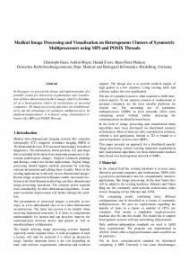
Supplemental Figure 1 – Small-world index of binary networks at different thresholds
●
6 ●
●
● ●
Cohort
SWI
4
HC PPMS
● ●
● ●
●
●
●
2
● ●
●
●
●
● ●
●
● ●
● ●
● ●
● ● ●
● ●
● ●
● ● ●
●
●
● ●
● ● ●
●
●
● ●
●
● ●
● ●
● ●
●
●
● ●
● ●
● ●
● ●
● ●
● ●
● ●
●
● ● ● ● ● ● ● ● ● ● ●
●
● ●
●
● ● ● ●
● ●
●
●
● ●
0
2.5% 5% 7.5% 10% 12.5% 15% 17.5% 20% 22.5% 25% 27.5% 30% 32.5% 35% 37.5% 40% 42.5% 45% 47.5% 50% 52.5% 55% 57.5% 60% 62.5% 65% 67.5% 70% 72.5% 75% 77.5% 80% 82.5% 85% 87.5% 90% 92.5% 95% 97.5%
Threshold
Boxplots for SWI = Small World Index. Computed for binary networks based on thresholds from 2.5% to 97.5% of raw weighted networks. HC = Healthy controls, PPMS = Primary progressive MS.
Supplemental Figure 2 - Node-specific graph metrics: Strength
Boxplots ordered by median values of nodes of Graw. Top: healthy controls, Bottom: PPMS
Supplemental Figure 3 - Node-specific graph metrics: Degree
Boxplots ordered by median values of nodes of Gbin. Top: healthy controls, Bottom: PPMS
Supplemental Figure 4 – Rich-club effect in mean connectomes
Weighted rich club organisation compared to benchmark values from 1,000 comparable random networks. Dots represent the ratio between the mean connectome and random networks. Yellow area represents 95%-CI from random networks, dots outside the area (red) can be considered significant. Top: strength of nodes in the mean connectome Graw. Middle: strength of nodes in the thresholded mean connectome Gbin. Bottom: degree of nodes in the mean thresholded connectome.
Supplemental Table: Comparison of different rich-club definitions
-0.08 (0.265) -0.20 (0.047)*
0.15 (0.101)
PPMS vs HC -0.06 (0.291) -0.26 (0.014)* 0.013*
Feeder
-0.04 (0.359)
-0.05 (0.344)
0.16 (0.092)
-0.1 (0.194)
-0.13 (0.141)
Periphery
0.03 (0.410)
0.09 (0.225)
-0.2 (0.049)*
0.12 (0.154)
0.22 (0.031)*
Six Top nodes Rich-club Feeder
0.01 (0.527)
-0.09 (0.225)
-0.08 (0.738)
0.13 (0.864)
-0.05 (0.326)
-0.16 (0.093)
-0.14 (0.115)
0.29 (0.009)*
-0.14 (0.109) -0.23 (0.026)*
Periphery
0.12 (0.158)
0.11 (0.175)
-0.21 (0.044)*
0.08 (0.257)
-0.07 (0.283)
-0.12 (0.153)
0.12 (0.156)
-0.12 (0.154) -0.28 (0.009)*
Feeder
-0.03 (0.389)
-0.06 (0.323)
0.18 (0.068)
-0.1 (0.194)
-0.21 (0.037)*
Periphery
0.07 (0.292)
0.07 (0.272)
-0.2 (0.047)*
0.13 (0.125)
0.25 (0.015)*
-0.04 (0.369)
-0.11 (0.175)
0.2 (0.05)*
Feeder
-0.02 (0.431)
-0.02 (0.447)
0.07 (0.279)
-0.1 (0.201)
-0.14 (0.123)
Periphery
0.06 (0.32)
0.07 (0.282)
-0.12 (0.156)
0.13 (0.125)
0.22 (0.029)*
-0.02 (0.442)
-0.12 (0.168)
0.04 (0.365)
0 (0.51)
-0.1 (0.195)
Feeder
-0.04 (0.369)
-0.11 (0.183)
-0.02 (0.574)
0.04 (0.623)
0.01 (0.527)
Periphery
0.03 (0.4)
0.11 (0.191)
-0.02 (0.437)
-0.05 (0.653)
0.08 (0.252)
EDSS Rich-club
A priori
Eight Top nodes
Ten Top nodes
Twelve Top nodes
Individual Eight Top nodes
SDMT
NHPTdom
NHPTndom
0.474
0.21 (0.035)*
Rich-club
0.254
Rich-club
0.022* -0.09 (0.216) -0.26 (0.014)*
Rich-club
0.539
Rich-club
0.235 0 (0.495)
-0.02 (0.435)
-0.02 (0.553)
0.01 (0.542)
-0.01 (0.473)
-0.01 (0.473)
-0.05 (0.344)
-0.08 (0.738)
0.02 (0.552)
-0.15 (0.098)
Periphery -0.02 (0.569) Rich-club
0.07 (0.272)
0.01 (0.532)
0.01 (0.469)
0.16 (0.084)
Feeder Individual Standard deviation
T25FW
0.997
0.2 (0.947)
0.11 (0.809)
-0.34 (0.998)
0.2 (0.962)
0.32 (0.997)
Feeder
-0.08 (0.248)
0.07 (0.718)
-0.29 (0.991)
0.15 (0.9)
0.07 (0.73)
Periphery
-0.1 (0.793)
-0.07 (0.728)
0.37 (0.999)
-0.21 (0.964)
-0.29 (0.994)
Associations between different rich-club definitions and clinical outcomes were estimated with Kendall’s tau. pvalues in brackets. Asterisk indicates p-values below 0.05. EDSS = Expanded disability status scale, T25FW = Timed 25 Foot Walk, SDMT = Symbol Digit Modality Test, NHPT = Nine Hole Peg Test, PPMS = Primary progressive MS, HC = Healthy controls.
1.
Smith SM, Zhang Y, Jenkinson M, et al. Accurate, robust, and automated longitudinal and cross-sectional brain change analysis. Neuroimage. 2002;17(1):479-489. doi:10.1006/nimg.2002.1040.
2.
Behrens TEJ, Berg HJ, Jbabdi S, Rushworth MFS, Woolrich MW. Probabilistic diffusion tractography with multiple fibre orientations: What can we gain? Neuroimage. 2007;34(1):144-155. doi:10.1016/j.neuroimage.2006.09.018.
3.
van den Heuvel MP, Sporns O. Rich-Club Organization of the Human Connectome. J Neurosci. 2011;31(44):15775-15786. doi:10.1523/JNEUROSCI.3539-11.2011.
4.
Griffa A, Baumann PS, Thiran J-P, Hagmann P. Structural connectomics in brain diseases. Neuroimage. 2013;80:515-526. doi:10.1016/j.neuroimage.2013.04.056.
5.
Welton T, Kent DA, Auer DP, Dineen RA. Reproducibility of Graph-Theoretic Brain Network Metrics: A Systematic Review. Brain Connect. 2015;5(4):193202. doi:10.1089/brain.2014.0313.
6.
Janssen RJ, Hinne M, Heskes T, van Gerven M a J. Quantifying uncertainty in brain network measures using Bayesian connectomics. Front Comput Neurosci. 2014;8(October):126. doi:10.3389/fncom.2014.00126.
7.
Humphries MD, Gurney K. Network “ Small-World-Ness ”: A Quantitative Method for Determining Canonical Network Equivalence. PLoS One. 2008;3(4):e0002051. doi:10.1371/journal.pone.0002051.
8.
Opsahl T, Colizza V, Panzarasa P, Ramasco JJ. Prominence and control: The weighted rich-club effect. Phys Rev Lett. 2008;101(16):1-4. doi:10.1103/PhysRevLett.101.168702.
9.
Collin G, Kahn RS, De Reus M a., Cahn W, Van Den Heuvel MP. Impaired rich club connectivity in unaffected siblings of schizophrenia patients. Schizophr Bull. 2014;40(2):438-448. doi:10.1093/schbul/sbt162.