International Journal of Future Computer and Communication, Vol. 4, No. 5, October 2015
Addressing Churn Prediction Problem with Meta-Heuristic, Machine Learning, Neural Network and Data Mining Techniques: A Case Study of a Telecommunication Company Abbas Keramati and Ruholla Jafari Marandi
Not so long ago data mining techniques have been being employed to grapple with the challenging and exacting customer churn problems in telecommunication service field [2]. Due to the mentioned heat of the competition in telecommunication market, these data mining techniques are mainly employed to tackle with the churn prediction issues which are receiving an unprecedented attention in the telecommunication industry and research (Luo et al. 2007). They are mostly applied, prevalently using the customer log-files or questionnaires, to come up with knowledge that it could discriminate those customers who are likely to churn. Although most of these data mining techniques use essentially different ways to achieve approximately same result, mentioned knowledge is totally worth-spending and beneficial for any today telecommunication company. Applying data mining techniques itself is a time consuming and so expensive. Data gathering, Data cleaning, and Data preprocessing in Iran rather immature telecommunication company also can be painstaking. Furthermore, the knowledge from data mining process is going to be used by company decision makers to make decisions - which should concerned as alterative and penetrative decisions and are about the most sensitive and attention-requiring matter in any telecommunication company, that is, Customers. Therefore, the more accurate and reliable knowledge is extracted by applying data mining techniques, the more proper and appropriate decision can be made by decision maker. Making appropriate decision about such a vulnerable matter needs tremendously certainty which can be achieved by a reliable knowledge. Incidentally, improper decision based on falsified, bias or flawed knowledge may bring about an unprecedentedly devastating situation where no one can make restitution. Contemplating previous researches, studies were concerned about churn determinants. They analyzed well-known churn determinates and verified them by using customer behaviors in telecommunication. Some attributes, including customer satisfaction, switching costs, customer demographics, tendency to change behavior, and service usage, have been commonly among churn determinants [3]. The rest of this paper is organized as follows: Section II gives an overview of other telecommunication business churn prediction. Section III describe the six technique describes in details. Section IV is devoted to show our experiences and the results of each classifier. Finally, Section V is for the conclusion and future trend.
Abstract—In order to survive in today telecommunication market it is essential to have the ability of distinguishing customers who are probable to switch into a competitor. Customer churn prediction is a means to address the complication and has become an important issue in Telecommunication business. In such competitive market a reliable means to predict customer future’s action would be regarded as priceless. To end, this paper has employed Meta-heuristic, Machine learning, Neural Network and data mining techniques including Genetic Algorithm, Particle Swarm Optimization, Support Vector Machine, Artificial Neural Networks, Decision Tree, and K-Nearest Neighbors so as to solve churn prediction problem. Using the data of an Iranian mobile company not only these techniques were experienced and were compared to each other, but also we drawn a parallel between some different prominent data mining software. However, the result indicates that this paper ANN performed the best with near 90 percent precision and recall. Index Terms—Telecommunication, churn prediction, data mining, meta-heuristics, ANN, KNN, SVM, decision tree, GA, PSO.
I. INTRODUCTION The mobile phone users during past years have outstandingly multiplied. Statistical report for the end of 2010 indicated that the number of mobile phone users in Iran has surpassed 70 million, more than 90% of the country population. Therefore, telecommunication market is on the point of being saturated. Mobile phone penetration rates for certain city have gone above 100%, which means there are more subscriptions than inhabitants. As a result, heat of the Competition in today telecommunication market is distinguishably high. Proposed products and service offerings are becoming more and more similar and replaceable. The fact that customers, in most of the cases, are able to self-centrically prefer a service provider better brings about the eroding of customer loyalty. Then, Iran telecom operators in near future need to start giving a great amount of attention to customer churn prediction and customer retention strategies otherwise they won‟t survive. Furthermore, it has been repeatedly shown that taking customer retention strategy is profitable for a company [1]. Manuscript received April 12, 2015; revised September 21, 2015. Abbas Keramati is with University of Tehran, Iran (e-mail:
[email protected]). Ruholla Jafari Marandi is with the Department of Industrial and Systems Engineering, Mississippi State University, United States.
doi: 10.18178/ijfcc.2015.4.5.415
350
International Journal of Future Computer and Communication, Vol. 4, No. 5, October 2015
II. LITERATURE REVIEW
customer churn prediction. Le et al. [7] focused on building an accurate and concise predictive model for the purpose of churn prediction utilizing a partial least squares (PLS)-based methodology on highly correlated data sets among variables. They presented not only a prediction model to accurately predict customers' churning behavior but also a simple but implementable churn marketing program. Their proposed methodology allows a marketing manager to maintain an optimal (at least a near optimal) level of churners effectively and efficiently through their marketing programs. In this research PLS is employed as the prediction modeling method. Briefly, in other studies, Kim and Yoon [8] identified the determinants of subscriber churn and customer loyalty in the Korean mobile telephony market. Owczarczuk [9] tested the usefulness of the popular data mining models to predict the clients churn of the Polish cellular telecommunication company. Author dealt with prepaid clients who are far more likely to churn, less stable and much less we known about them. The results of his research showed that linear models, especially logistic regression, are a very responsive choice to mode churn of the prepaid clients. Coussement and Poel [10] developed a DSS for churn prediction. It tries to integrate free-formatted, textual information from customer emails with information derived from the marketing database. They investigated the beneficial effect of adding the voice of customers through call center emails – i.e. textual information – to a churn-prediction system that only uses traditional marketing information. Their findings proved having unstructured, textual information added into a conventional churn-prediction model will result in a significant increase in the prediction performance. Sweeney and Swait [11] investigated the important additional role of the brand in managing the churn of current customers of relational services. Their research leaded to the enhanced understanding that the brand has a significant role to play in managing long-term customer relationships, and details how the usual tools of customer relationship management, satisfaction and service quality, relate to brand credibility. Their results from samples of retail bank and long distance telephone company customers indicated that brand credibility serves a defensive role. One can see that data mining techniques, such as Decision Tree, Neural Network, Support vector machine, Bayesian Belief Networks, and Regression, have been prevalently employed in telecommunication customer churn prediction studies. Nevertheless, just a few of them have gone through the process of tuning these techniques parameters in order to compare them to each other. In this paper we have experience, tuned, and compare six prominent classification techniques namely Genetic Algorithm, Particle Swarm Optimization algorithm, Decision Tree, Artificial Neural Network, K-Nearest Neighbor and support Vector Machine. Apart from that we used ANOVA to compare and differentiate mentioned techniques. We also have compared the performance of some of the well-known data mining software such as R, Weak and MATLAB.
An Accurate and reliable prediction of churn customer is important to develop appropriate retention strategies. Huang et al. [2] proposed a method based on ordinal regression to predict time of churn and tenure of customer in mobile telecommunication industry. They treated Customer tenure as an ordinal outcome variable and take advantage of ordinal regression to make a model out of it. Their results showed ordinal regression could be an alternative technique for survival analysis about the prediction of mobile customers‟ churn time. This paper has been the first study, its authors claimed, to use ordinal regression as a potential technique for modeling customer tenure. Zhang et al. [3] investigated the effects of interpersonal influence on the accuracy of customer churn predictions and proposed a novel prediction model that is based on interpersonal influence and that combines the propagation process and customers‟ personalized characters. The comparison between results of traditional attributes-based models, network attributes-based models and combined attributes models proved that incorporating network attributes into predicting models can greatly improve prediction accuracy. Hung et al. [4] intended to illustrate how to apply IT technology in order facilitate telecom churn management. Their main goal, unlike to the most of other churn analysis research, was not to predict customer‟s churning attitude so as to decide what measures should be taken about the retention. However Authors opted for decision tree, neural network and K-means cluster among data mining techniques to come up with a churn predictive model. They had categorized their churn attributes into three segments according to their billing amount (to assess „customer value‟), tenure month (to appraise „customer loyalty‟), and payment behaviors (to engage „customer credit risks‟). Normally in churn analysis research the effective churn deterministic variables are chosen by running a regression model or other means, however, they simply used expertise‟s outlook in order to discern effective churn deterministic variables. Task of using association rules is to reduce a large amount of information to a small and more understandable set of statistically supported statements [5]. Few studies have considered or illustrated the pre-processing step during data mining whose aim is to filter out unrepresentative data or information. The aim of Tsai and Chen [6] was to examine whether association rules can be adapted in the data pre-processing stage to reduce a large amount of information to a small and more understandable data variables in order to improve the prediction performance of neural networks and decision trees. They, after discussing some preprocessing steps, presented the important processes of developing MOD customer churn prediction models by data mining techniques. Their study contains the pre-processing stage for selecting important variables by association rules and also it was consisted of the model construction stage by neural networks (NN) and decision trees (DT). Their experimental results showed that using association rules allows the DT and NN models to provide better prediction performances over a chosen validation dataset. Authors also investigated the combination of the data reduction and model development steps using data mining techniques for the problem of MOD
III. SOFT COMPUTING TECHNIQUES A. Genetic Algorithm 351
International Journal of Future Computer and Communication, Vol. 4, No. 5, October 2015
resulted in their popularity between data mining practitioner. They are wonderful means to predict objects categories (classes), taking into account the values of predictor attributes. The decision tree‟s very suggestive visualization and flexibility make it practically attractive. As an experimental exploratory technique, especially when other techniques have failed, decision trees may prosperously be employed, being picked rather than other classifications models. Decision tree is one of the alleviation for all problems which has been caused in the mass storage era. It has gained popularity because of its conceptual transparency. Decision trees have been found useful in building knowledge-based experts systems [14].
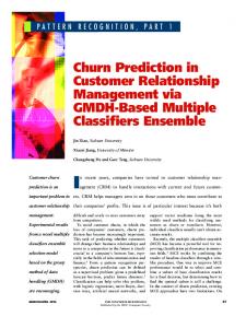
Genetic Algorithm (GA) is a progressive and highly adaptive meta-heuristic algorithm which was invented by Holland and his colleagues in the 1965 [12]. During these few decades researchers has proven to be highly absorbed into using the methodology. Just like any other recognized and highly in used algorithm it has gone through modification and alteration. We can introduce GA essence by the chromosome concept, its initialization, crossover, and mutation operators. GA is a highly adaptive algorithm; one is able to inspire the spirit of his or her considered problem into the procedure of the algorithm by simply defining its chromosome and fitness function. Though there has been a load of efforts and research for the sake of promoting GA operators, the role of defining eligible and qualified chromosome has an impacting influence on the performance of GA. GA chromosome has the most adaptable essence among the other GA concepts, moreover, it can be claimed that it is the superiority point of GA in comparison with the other approaches. Binary chromosome is the simplest kind to define and to be treated by GA operators (Mutation, crossover). The genetic algorithm flowchart is represented in Fig. 1.
D. Artificial Neural Network Artificial neural network (ANN) is an information processing mechanism which is inspired from biological nervous systems. ANN comprises some interconnected elements, or neurons, working together as one soul to solve specific problems. The structure of an ANN is determined by both the inter-neuron connections‟ arrangement and the nature of these connections. The way of training or adjusting the strengths of aforementioned connections so as to achieve a desired overall behavior is known as its learning algorithm [15]. ANNs are well-known for their well-established empirical modeling power. Their most outstanding feature is their ability to learn automatically themselves from an available data in order to provide a means for predictions. They also are able to somehow impose blind (hidden) insights into the hidden relationships [16]. ANNs can be categorized into two different groups considering their structures: Feed-Forwards and Recurrents. A Feed-Forward network‟s neurons are grouped into input, hidden and output layers. Feed-Forwards networks can be recognized by unidirectional arrows which flow from input layer through the output, not connecting neurons in a same layer but connecting them from previous layer just to the next one [15]. A simple Feed-Forward network with one hidden layer is presented in Fig. 3.
B. Particle Swarm Optimization Particle swarm optimization (PSO) is a progressive and evolutionary computation algorithm introduced by [13]. The algorithm has been widely in use over these few decades. Although their earlier algorithm has gone through some alteration and modification by other researcher or themselves, its essence has remained intact and the algorithm has been outstandingly in use. The algorithm has some similarity to other evolutionary algorithms, it is among population-based search algorithm. Among others, its initialization is entirely randomized. Its unparalleled difference is, however, each individual, called particle, efficiently keeps and uses its own-achieved best answer (pbest) during the competition. We have depicted the procedure of PSO algorithm by means of flowchart in Fig. 2. There are two equation used in this figure. The equations and their definition are available as follow:
E. Support Vector Machine SVM was first introduced by Vapnik. The basic version of classifier would deal with two-class problems in which the training data divided into two classes using a hyperplane which is defined by a number of support vectors. It was based on the Structural Risk Minimization (SRM) principle stated in computational learning theory. The basic idea behind supervised learning methods is to learn from observations. SVM endows us with a binary classifier by actually finding optimal separated hyperplanes through nonlinear mapping of the input vectors into a high-dimensional feature space. Based on support vectors, SVM constructs linear models to estimate the decision function by taking the advantage of the nonlinear class boundaries. In case the training data is linearly separable, SVM results in the optimal hyperplane with maximum distance between the hyperplane and those training sample which are closest to the hyperplane. These samples with minimum distance to the hyperplane are called support vectors. SVM only uses support vectors so as to find the hyperplane and so all other training samples are irrelevant.
Vid C0 Vid C1 r ( Pbid X id ) C2 r (Gbd X id ) (1)
X id X id Vid
(2)
Definition of variables in equations 1 and 2 are as follow: X: the position of population i: index for each particle d: index for each dimension v: velocity r: a randomized number with uniformly distribution [U(0,1)] . Pb: the position of pbest Gb: the position of gbest C0, C1, and C2: constants to be specified by practitioner. C. Decision Tree This One of the most popular and prevalently in-used classification techniques in the data mining process is decision trees. Their exceptional flexibility and understandability are their greatest advantage which has 352
International Journal of Future Computer and Communication, Vol. 4, No. 5, October 2015
the label will define their classes. The simplest case is when the class labels are binary but still it is applicable on arbitrary class numbers.
When the data is not linearly separable SVM uses nonlinear machines to find a hyperplane based on the minimum training error criterion [17]. Specify: Chromosome encoding Structure / chromosome decoding function / fitness function / N of population / N of Iterations / keeping, crossover, mutation, new percentages/ mutation rate / stoppage criteria
Specify: Number of population Fitness function Stoppage criteria C1 C2 C3
Initialize population by randomly filled chromosome
Initialize population: Specify some random numbers for each particle’s position and some others for their velocities and set the p-best for each of them as the same position
Decode each chromosome and in population and calculate the fitness values
Sort the population with regard to their fitness function
Compute Fitness: Calculate the fitness value of each particle with regard to its position
Send as many as pel*Population of best chromosome into next generation
Update pbest: If the current value for each individual is better than its pbest update its pbest position and value instead of current position
Choose pairs of chromosome to undergo the crossover and send the results into next generation
Update gbest: Update gbest position and value with the most eligible particle’s position and value
Choose chromosomes to undergo the mutation and send the results into next generation
YES
Update position and velocity for each particle using the two updating equation
Is number of chromosome adequate in next generation?
NO
Is stoppage criteria met?
Compensate for the shortage by new random chromosome
NO
Yes Is stoppage criteria met?
Report gbest and the answer YES
Fig. 2. PSO flowchart.
Report gbest and the answer
Fig. 1. GA flowchart.
F. K-Nearest Neighbor Among various classification techniques, most of them rely on many assumptions made over data but in practical cases only few of them are applicable. Beyond such methods another type of learning algorithms named non-parametric learning has been introduced. These types of algorithms make no assumption on the data and therefore they are applicable on many real world problems. K-Nearest Neighbors (KNN) is one the most applicable and useful non-parametric learning algorithms. KNN may be known as a lazy algorithm, that is, all training data is used at testing phase. In fact there is no training phase and all data points are used directly in test phase, so these all points need to be used when it is to be tested [18]. KNN uses the distance between records so as to use it for classification. In order to measure the distance between the points, KNN assumes that these points are scalar or multidimensional vectors in feature space. Euclidean distance is one the most commonly used measuring methods used in KNN. All data points are vectors of feature space and
Fig. 3. Feed-Forward Network with one hidden layer.
IV. TUNING AND EXPERIENCES A. The Dataset We used the dataset which was randomly selected from an operator call-center‟s database over a 12-month period. The dataset contains 3150 customer data such as number of Call Failure, number of Complains, Subscription Length, Charge 353
International Journal of Future Computer and Communication, Vol. 4, No. 5, October 2015
Amount, Seconds of Use, Frequency of use, Frequency of SMS, Distinct Calls Number, Age Group, Type of Service, Status, and Churn. Obviously the class attribute is Churn [12]-[20]. Looking into data, we saw there were 495 records with the class label churned and the rest, i.e. 2645, were non-churned. For the sake of keeping our experiments in proper randomization environment, for each single block we randomly select 70% of dataset for training set and the rest for
the validation process, with respect the proportion of 2 distinct classes. In another word, our every single experiment was done by a training set with 347 records labeled Churned and 1858 non-churned ones (totally 2645 records). Also all of this paper validation process has been performed by 148 churned and 347 not-churned classes (totally 495). Using the mentioned process, we prepared 3 blocks in order to run and compare experiments.
Fig. 4. A part of GA chromosome.
It goes without saying that since the fitness function is cost the algorithm job is to come up with the best variable which can minimize the error. After delineating the fitness function for the PSO algorithm there are some other issues to be decided for before using. First, one should clearly specify the number of variable and the range they are allowed to alter. For this case, since there are 11 predictor in the equation model and each of them needs two variable one for its α and the other for its β and there is one α0 we need 25 variable all together. We assigned them freely to roam between -25 and 25. The number of population which were used was 25. So as to tune the other factors of algorithm we experienced and saw its demeanor. At the end, we specified 40, 1, 0.2 and 0.2 respectively for number of iterations, C0, C1 and C2. The most imposing feature of a GA is its chromosome structure. Upon decoding of a GA‟s chromosome, one can extract the variable to calculate the algorithm fitness function. Therefore, the introduction and the decoding methodology of our chromosome is presented in this part. Fig. 4 how a part of the chromosome structure and at the same time represent the decoding function. One can see that the first row is for specification of αs, as well as second row which is for βs. The chromosome is to be continued from left side with the same structure up until the part related to α11 and β11. The decoding procedure for each part of the chromosome is represented in the Fig. 4. After the representation of chromosome structure, the crossover and mutation operators need to be described. For crossover, after being parted, the two rows undergo the traditional single break crossover and then reunited together again. Also, for Mutation, the neurons are to be changed from zero to one or vice versa if they are indicated by the random selection of mutation operator. The number of these random selection is decided by a mutation rate which is one of the factor can influence the algorithm behavior. Moreover, the algorithm needs a procedure to select pairs of chromosomes for crossover and chromosomes for mutation. The procedure used in this study was the simplest one: random selection between the chromosomes in the current generation.
B. Evaluation Measures In terms of binary classification there are known measures to check the accuracy or performance of a classifier. They range from as simple as accuracy or misclassification measures to precision and recall which give more insightful take about the performance of classifier. Obviously there is not a better or more eligible classifier for all the cases and a data mining practitioner normally choose one of them insightfully. In another word Understanding them will make it easy to grasp the meaning of the various measures. In this paper we have used the three measures namely, Recall, Precision, and F-Score. It is noteworthy to say that F-Score is actually a combination of the other two. C. The Dataset GA and PSO are two optimization algorithm so they do not have the capability of predicting and classifying innate in them. Therefore, for one to be able to use them for such purposes it is vital to inspire matter to the process. One of the part that PSO and GA can be affected so as to be adapted to be used as classifier is their fitness function. If we are able to define a fitness function by which the algorithm can improve a model parameter we can actually claim that we have been able to make the optimizer algorithm a classifier. In light of incorporating such model in the two algorithm, we opted for the following equation as a predictor for Churn analysis.
churn 0 11 2 2 3 3 4 4 5 5 6 6 7 7 8 8 9 9 10 10 1111
(3)
In this equation, Ps are the representation of the model predictors. As we saw at the Dataset section we had eleven predictors and one class. The class column is the one we are striving to predict and here our case is predicting whether one person would churn or not. αs and βs are the variable to be specified by the algorithm. The process we used was the manipulation of the algorithms fitness function. We defined it the error of the model if it were the predictor for the train data. 354
International Journal of Future Computer and Communication, Vol. 4, No. 5, October 2015
neurons was 0.845.
However, exactly the same as PSO we experienced Genetic Algorithm and tuned it by trial and error. We finally decided that Genetic algorithm with the represented equation model and the chromosome and the operators can run sufficiently by respectively 25, 100, 0.15, 0.6, 0.15 ,0.1 and 0.3 for number of population, number of iterations, keeping percentage, crossover percentage, mutation percentage, new chromosome percentage and mutation rate. TABLE I: ANOVA TABLE FOR DT 1 2 RE PE RE PR MATLAB 0.83 0.80 0.82 0.77 R (Part) 0.40 0.97 0.75 .78 R (rparty) 0.78 0.75 0.77 0.73 WEKA (AD.Tree) 0.61 0.73 0.36 0.92 WEKA (BF.Tree) 0.79 0.86 0.75 0.84 WEKA (FT) 0.78 0.86 0.83 0.79 WEKA (J48) 0.83 0.80 0.85 0.77 WEKA (LADTree) 0.69 0.70 0.66 0.76 WEKA (LMT) 0.81 0.88 0.84 0.81 WEKA (NBTree) 0.77 0.83 0.81 0.77 WEKA (Random 0.79 0.90 0.83 0.90 Forest) WEKA (Random 0.75 0.79 0.82 0.82 Tree) WEKA (REPTree) 0.78 0.81 0.78 0.71 WEKA (Simple 0.85 0.85 0.75 0.87 Cart) Experiments
F. SVM As it mentioned before SVM has several parameters to be decided on. So as to decide we applied cross-validation tuning for SVM parameters. The best F-Score achieved by SVM was 0.8383. The summery table for the final result of different kernel on test data is Table IV. Our experience proved that the best tuning of parameter for this paper classification problem is applying Polynomial kernel with order of 4.
3 RE 0.82 0.51 0.77 0.41 0.77 0.75 0.71 0.69 0.78 0.67
PR 0.83 0.93 0.73 0.82 0.86 0.86 0.90 0.79 0.89 0.93
0.81
0.94
0.79
0.85
0.81
0.84
0.83
0.88
Kernel Type RBF MLP Polynomial
G. KNN The other data mining technique has been applied to this paper dataset is KNN. It is among those techniques which desperately needs beforehand tuning. The tuning parameters of KNN model using cross-validation is presented in Table IV. This table reports the F-Scores calculated using the number of neighbors and method of distance calculation. The results showed that using cosine distance method along with 1 neighbor has led to the best F-Score gained by KNN.
D. DT We constructed the following completed block design ANOVA, Table I, first to examine the responsiveness of decision trees handling churn prediction problem, and then to compare the some software performances. It goes without saying that the difference between the software in terms of Decision Tree algorithm is the source of difference. There are three values for each cell in the ANOVA table which are respectively, from the left, the value of recall (RE) and precision (PR) measure for each decision tree run.
1 Euclidean City Block Cosine Correlation Euclidean City Block Cosine Correlation
0.747
0.824
0.841
0.83
0.843
0.829
8
0.841
0.783
0.857
0.828
0.877
0.847
9
0.85
0.83
0.758
0.854
0.825
0.87
10
0.817
0.845
0.828
0.852
0.828
0.857
11
0.798
0.795
0.841
0.871
0.852
0.775
12
0.814
0.86
0.783
0.858
0.836
0.86
TABLE IV: KNN TUNING 2 3
0.5119 0.5544 0.7343 0.7178 6 0.3695 0.4219 0.7119 0.7148
0.5119 0.5544 0.7343 0.7178 7 0.3592 0.4351 0.7079 0.6920
0.4170 0.4981 0.7168 0.7247 8 0.3362 0.4309 0.7113 0.7067
4
5
0.4170 0.4747 0.7189 0.7128 9 0.2819 0.3821 0.7317 0.7298
0.3968 0.4615 0.7007 0.7083 10 0.2489 0.3739 0.7234 0.7298
H. Comparison Except for decision tree, other techniques‟ demeanors were observed and consequently were tuned to be adapted to the spirit of churn prediction problem in their best ways. This paper‟s aim is to compare and contrasts the performances and the demeanors of all the introduced soft computing methodology. Table IV shows a complete block design table in which all of the introduced soft computing techniques results (F-Scores) for the aforementioned blocks are presented. Except for block 3 and 5 in which respectively SVM and GA has slightly outperformed ANN, it has been ANN that has had the best results. Table V and Table VI are respectively summery and the ANOVA complete block design analysis result for the techniques. The ANOVA results, Table VII, as it could be predicted, have rejected the hypothesis that the performances of different techniques approaching Churn prediction are similar (p-value