ADJOINT RADIOSITY BASED ALGORITHMS FOR RETRIEVING TARGET REFLECTANCES IN URBAN AREA SHADOWS Christoph Bore1a, Kenneth Ewalda, Mark Manzardo, Charles Wamsleya and John Jacobsonb a
Ball Aerospace & Technologies Corp., Fairborn, OH 45324, USA b NASIC, Wright Patterson AFB, OH 45433, USA
[email protected] KEY WORDS: Atmospheric correction, reflectance retrieval, shadowing, urban, LIDAR, illumination, radiosity ABSTRACT: Current hyperspectral target finding algorithms require the matching of spectral reflectance signatures to measured radiance spectra. Before spectral matching, the measured sensor radiances are converted to apparent surface reflectance by a step called “atmospheric correction”. Several atmospheric correction methods (ACM) exist such as FLAASH, ACORN, 6S, MODFULL, ATCOR and others. They all assume that the surface material is fully illuminated by the sun and sky. Many ACMs include adjacency scattering effects and some also attempt to account for scattering contributions from nearby surfaces. Thus current ACM’s make finding desired target signatures possible as long as the targets are out in the open and illuminated by the sun. Targets in shadow, however, are much more difficult to find. For example a target in the shadow of a building is illuminated by an unknown mixture of skylight (clear sky and clouds) and scattered light from surrounding areas, which may be illuminated or shaded. To handle this more difficult case we proposed to use the adjoint radiosity method. In this paper we will show simulations of complex urban scenes and how illumination changes the appearance of objects. We discuss a method to retrieve the illumination in complex environments to improve estimates of the background and target reflectances. There are two major benefits of this research. First, we improve the matching of target signatures in complex environments, e.g. in urban and under vegetation. Second, change detection will be easier since given a 3-D representation of the environment we are able to create re-lighted views of a scene to correct for different illumination conditions.
1. INTRODUCTION It is commonly assumed that the retrieval of surface reflectance values involves only correction of the atmospheric terms, the transmission and path radiance. Radiative transfer based atmospheric correction algorithms such as ATREM [6], FLAASH [1], 6S [11], ATCOR [10], HATCH [9] and ACORN [2] also take the sky’s spherical albedo into account and may remove the atmospheric adjacency effect. In a typical radiance model this (6S) takes the following form:
Lm =
E0
π
cos θ s
τ s (θ s ) {ρτ direct (θv )+ < ρ > τ diff (θv )} + Lp 1− < ρ > s
(1)
where: Lm is the measured radiance, ρ is the Lambertian surface reflectance, s is the spherical albedo of atmosphere, is the adjacency filtered reflectance, E0 is the solar irradiance, τs is the transmission from sun to surface, τ=τdirect+τdiff, where τdirect is the direct and τdiff is the diffuse transmission from ground to sensor, and Lp is the path radiance. The surface reflectance is then obtained by:
ρ=
Lm − L p ρ ac where ρ ac = π . 1 + ρ ac s E0 cos θ sτ s (θ v )τ (θ v )
The current radiance models used to solve for surface reflectance assume that: • • • •
The surface is illuminated only by sun and skylight and its contribution is constant over the surface. No clouds are allowed, since they would add additional illumination terms and make the illumination dependent on the pixel position. The scattering from adjacent 3-D surfaces such as trees and buildings is neglected. The surface normal is vertical, e.g. this requires a “flat Earth”.
To demonstrate the importance of considering the illumination from the environment we put together an elaborate MATLAB tool based simulation. The following assumptions were made: • •
The atmosphere is modelled using MODTRANTM. The observer is above the atmosphere at 99km. The sun zenith angle is 30 deg. The model atmosphere is chosen to be mid-latitude summer with rural aerosols and 23 km visibility. The scene modelled consists of a vertical wall with 50% reflectance oriented such that it is in shade and the horizontal surface also has a reflectance of 50%. The irradiance on the wall is approximated by the sum of the sky radiance integrated over a halfhemisphere and the radiance from the horizontal surface and no multiple scattering between the wall and the surface is considered.
Fractional contribution to total radiance
The radiance at the sensor for a point on the horizontal surface in the shadow of the wall is the sum of: • The path radiance Lpath, i.e. the scattered solar radiance within the atmosphere reaching the sensor. • The reflected down-welling sky radiance Ldown, i.e. the radiance from the half-hemisphere reflected from the horizontal surface and reaching the sensor. • The reflected radiance Lenvironment from nearby surfaces reaching the sensor, i.e. the shaded wall which receives light from the sky and from the illuminated horizontal surface. • The atmospheric adjacency radiance Ladjacency which consists of radiance scattered into the line of sight from nearby surfaces and radiance from light scattered by the surrounding horizontal surface and reflected by the atmosphere and then again by the horizontal surface.
Ladjce ncy
Lenviro nment
Ldown Lpath
Figure 1 The fractional contribution for a pixel in shade near a vertical wall from the path radiance Lpath (light blue), reflected downwelling sky radiance Ldown (dark blue), scattering from the environment (vertical wall) Lenvironment (gray) and atmospheric adjacency Ladjacency (green). In Figure 1 the fractional contribution of each of the above terms is shown as a function of wavelength. Notice that the fractional contribution of the environmental radiance Lenvironment grows from about 20% in the visible to up to 80% in the SWIR. Thus for shaded pixels, the current model based atmospheric correction algorithms are commonly considered unusable. And therefore new algorithms are necessary which take non-ideal illumination conditions for surfaces in shade and also for scenes with partial cloud cover. In a complex 3-D scene the irradiance is different for each visible point in the scene since it depends not only on the direct solar illumination and sky radiance but also the multiple scattered radiances from nearby surfaces. An interesting case occurs in the near infrared (NIR) where shadows can be brightened under vegetation by the high transmission of NIR light through leaves and in urban scenes by bright clouds. In the second section of this paper we describe the fundamentals of the adjoint radiosity method. In the third section of this paper, we will show the effect of illumination in a very simplified urban environment. 2. FUNDAMENTALS OF THE ADJOINT RADIOSITY METHOD Computer graphics originally was developed to synthesize images from given reflectances, geometric models and realistic illumination. One of the most successful methods to be used for this purpose is the radiosity method introduced in 1984 to computer graphics [8] after being used for decades in thermal engineering. It is now used in every advanced rendering package and even in computer games. Since current highly realistic scenes easily contain hundreds of thousands and sometimes up to several hundred million polygons, there are many shortcuts used which limit the quantitative applicability of the radiosity results. Currently most radiosity implementations just create pretty pictures, consider only diffuse reflection and no transparent surfaces. The progressive radiosity method shoots energy only from brightest surfaces and can take a long time to converge. More recent approaches like photon mapping and Monte Carlo raytracing can introduce noisy artifacts. However the lack of accuracy and the algorithmic shortcuts limit the applicability of the radiosity method to remote sensing problems where transmissive surfaces exist for vegetation and many surfaces are bright. Some of resulting shortcomings are listed in the primary author’s papers ([3][4][5]) that have used the radiosity method to calculate scattering in vegetation canopies, terrain and atmospheres. These papers also contain reviews of the radiosity model as adapted to remote sensing and should be consulted by readers interested in more details.
In recent years the computer graphics community has realized also that it might be possible to reverse this process, i.e. to estimate the scene illumination given an image, geometry and surface reflectance properties [12]. If this can be done, it is a very useful technique to improve the “believability” of digital special effects in movies, e.g. insertion of computer generated objects. This new area is sometimes called inverse rendering, inverse global illumination and/or adjoint radiosity. Note, that the inverse rendering approach is very similar to what is usually attempted in remote sensing, i.e. estimating illumination and surface reflectances from a measured radiance image. For the method to work well, however, it is necessary to obtain accurate 3-D geometry information about the imaged scene. The adjoint radiosity method is still a research topic in computer graphics where the need often arises to embed computer generated objects, with a realistic re-lighted illumination field, into existing images and movies or embed a relighted human into a lighted computer generated environment. The human vision system can detect when the wrong illumination field is used. The current approach uses light probes which consist of spheres which are placed where the computer generated object is to be placed. Diffuse scattering spheres capture the low-frequency content of the illumination field. Mirrored surface spheres are used to capture distant and bright light sources. Multiple filming is required to create the necessary frames, e.g. a scene without a light probe, a scene with a diffuse ball and a mirror ball. Due to the cost of all these special steps, researchers have started to develop methods to infer the illumination directly from the film frames themselves. The traditional forward computer graphics rendering approach assumes a 3-D environment geometry, a reflectance model for each surface and an illumination field to generate highly realistic images. In remote sensing, however, we have the “image” as measured by a sensor and can obtain information about the geometry from digital elevation models (DEM’s) and/or Light Detection And Ranging (LIDAR) data. Under perfectly clear and uniform conditions we can model the illumination from the sky using radiative transfer. The big problem is how to determine the surface reflectance from the measured data in shaded pixels and under partly cloudy conditions. Figure 2 shows how we envision the process of retrieving reflectances from measured radiances after performing an illumination correction using the adjoint radiosity approach. The advantage of the adjoint radiosity approach is that after the atmospheric correction, the illumination can be determined on a pixel-bypixel basis for each point using the 3-D information.
HSI Sensor
DN
Calibration
Sun Lm(x,y,λ)
Atmosphere
Atmospheric Correction Lsky(θ,φ,λ) 3-D model
Lsurf(x,y,λ) Illumination Correction
ρ(x,y,λ) Figure 2 Concept of reflectance retrieval after performing an illumination correction using the adjoint radiosity method. 3. ILLUMINATION SHADED STREET CANYON MODEL In this section we will present a simple 2-D radiosity model of a corner which represents a typical geometric situation found in an urban setting. We will compute the radiosity of surfaces in shade and in direct sunlight for different geometries and illumination angles. In a previous paper [6] we presented a simulation of a city under a realistic sky illumination scenario, described a fast method to compute the hemispherical sky views from any point on a digital elevation model (DEM) using a shadow volume technique and set up the shaded street corner radiosity problem similar to our other models, e.g. the single and n-layer canopy models which are described in [3] and [4]. The model is a 2-D model and the geometry is shown in Figure 3.
θsun
(a) θsun
(b)
B3
A
C
B1
3
1
H
B3b
B1
3
1
S3
D
B
B2a
B2b 2
B2b
H
B3a
2
S2=tan(θsun
W
W
Figure 3 Geometry of the street canyon radiosity model. The walls (1) and (3) have height of 1 and the horizontal surface (2) has a width w. There are two possible illumination cases (a) the sun casts a shadow of wall 1 on the horizontal surface 2 and (b) the wall casts a shadow on the vertical surface 3. Rather than defining a separate source for sun and sky light which would make the analytical model too complex, we calculate the first interaction of the sources with the surfaces and label them with surface averaged irradiances Ei. Once the length averaged radiosities are obtained, they can be split up into radiosities in the sunlit and shaded part. For the surface averaged radiosities {Bi, i=1,2,3} can be written as:
B1 = ρ1 [ E1 + F21 B2 + F31 B3 ] = ρ1 [ E1 + aB2 + cB3 ]
B2 = ρ 2 [ E2 + F12 B1 + F32 B3 ] = ρ 2 [ E2 + bB1 + bB3 ] .
(2)
B3 = ρ3 [ E3 + F13 B1 + F23 B3 ] = ρ3 E3 + cB1 + aB2 ] The total irradiance E0 is split into a direct term with a fraction (1-fsky) coming from sun with an angle θs relative to nadir and a diffuse term with a fraction fsky which is assumed to be not dependent on incidence angle. The solution of (2) is obtained by solving the following matrix equation:
− a ρ1 −c ρ1 B1 1 T −b ρ 1 −b ρ 2 B2 = ρ 2 −c ρ3 −a ρ3 1 B3 I − ρT F B = F ⋅ B = ρT ⋅ E 0
E1 E 2 E3 .
(2)
The irradiance on surface 1 is only due to sky light which is assumed to be a fraction fsky of the total irradiance E0 multiplied by the view factor Fsky,1. The irradiance on surfaces 2 and 3 is equal to the solar irradiance averaged over the total width W (if illuminated) and the fraction of sky illumination multiplied with the view factors Fsky,2 or Fsky,3 from the sky to surface:
E1 = E0 f sky Fsky ,1
( ) (1 − f ) sin θ
E2 = E0 fillum 2 1 − f sky cos θ s + E0 f sky Fsky ,2
E3 = E0 fillum3
sky
s
(4)
+ E0 f sky Fsky ,3
The fractions of sun illuminating surfaces 2 and 3 are given as:
W H ,else 1 − tan θ ,else s W H tan θ s f illum 2 (θ s ) = and f illum 3 (θ s ) = 0, if θ > tan −1 W 1,if θ < tan −1 W s s H H
(5)
The view factor Fij is the fraction of light from surface i which arrives at surface j and for this 2-D case can be computed using Hottel’s crossed string method (see [4]). Hottel found that the view factor between two non-intersecting line segments AB and CD (e.g. see Figure 3 (a)) is given by the sum of the lengths of the crossed strings minus the non-crossed strings divided by the length of segment AB:
FAB →CD =
AD + BC − AC − BD 2 AB
The view factors can be derived as a function of the horizontal plane width W and wall height H with the following equations and simplifications and expressing the terms a, b and d as a function of c:
a = F21 = F23 = Fsky ,1 = Fsky ,3 = b = F12 = F32 =
H +W − H 2 +W 2 2W
=
H (1 − c) 2W
H +W − H +W 2 1− c = 2H 2
H 2 +W 2 −W c = F31 = F13 == H d = Fsky ,2 = F2, sky =
(6)
H 2 + W 2 − H H (c − 1) = +1 W W
Using (2)-(6) we can solve for the average surface leaving radiosities B1, B2 and B3 using at least three approaches. The first approach is to invert the view factor matrix F and find the solution as: T −1 B = ρ F E
(7)
The second is to solve the radiosity equations analytically which can be done using a symbolic mathematics program such as Xmaxima. The third is to iteratively solve the radiosity equations (2) starting with [B1, B2, B3] 1=[E1, E2, E3] using the Gauss-Seidel method. At each iteration an additional multiple reflection takes place and the iteration is stopped when the differences of the radiosity values between iterations reaches a small value. This method is practical when a large number of radiosities need to be solved and a matrix inversion becomes too computationally exorbitant. Note also that in practice the view factor matrix for a 3-D problem is very sparse which makes storage and solution much more tractable. If a surface is partially sunlit, then the solution needs to be split between the illuminated and shaded surface. The radiosity in the shade is given by the sum of the reflected sky radiance and the reflected radiance from other surfaces. If surface 2 is partially sunlit, we compute the radiosity B2a in the shaded part of surface 2 which is given by the reflected diffuse sky illumination and the multiple scattered light from the surrounding surfaces which we call B2multi. The term B2multi is computed as the difference between the radiosity B2 and the surface averaged irradiance which includes sun and sky light. If surface 2 is partially sunlit, then the radiosity B2b in the sun-lit part is the sum of the reflected solar and diffuse sky irradiance and the multiple scattered radiosity B2multi:
B2 multi = B2 − ρ 2 E2
B2 a = ρ 2 E 0 f sky Fsky ,2 + B2 multi
(8)
B2b = ρ 2 E0 (1- f sky ) cos θ sun + ρ 2 E 0 f sky Fsky ,2 + B2 multi , if f illum 2 > 0 And similarly for surface 3 if it is partially sunlit, then the radiosity in the shade is B3a and in the sunlit part is B3b is given by:
B3multi = B3 − ρ3 E3
B3a = ρ3 E 0 f sky Fsky ,3 + B3multi , if f illum 3 > 0
(9)
B3b = ρ3 E0 (1- f sky )sin θ sun + ρ3 E 0 fsky Fsky ,3 + B3multi The above approach was introduced in [3] has the advantage that only three surfaces and three equations are necessary and can treat all illumination cases which are dependent on the sun zenith angle and canyon dimensions. The current computer graphics radiosity implementations actually use the shadows cast by point light sources onto the polygons to sub-divide the polygons further and thus create illumination dependent solutions. Numerical comparisons of solutions for a model with three surfaces instead of two for a model with two opposing square plates where the lower plate is partially shaded have shown that this can be done with little loss in accuracy. Since the geometry and approach is similar (surface 2 is not used), we assume that this also holds true for the street canyon model. In Figure 4 we show a visualization of the computed radiosities for the two cases shown in Figure 3. The geometry of the street canyon (W=1 and H=1) is shown using the thickest lines. The slanted dash-dot line shows the shadow line cast from the left wall (surface 1) onto the horizontal surface 2. In this case the sun zenith was 30 and 60 degrees. The numerical value of the radiosities is printed and also visualized as rectangles which are plotted to the left and right of surfaces 1 and 3 and below surface 2. The model
calculations assumed E0=1. The broken lines inside the rectangles show the multiple scattered terms B2multi and B3multi. The diamond symbols indicate the “truth”.
Figure 4 Visualization of the inverted “street canyon” radiosity model with randomly selected reflectances and sky fraction for the case (a) and (b) of Figure 3. The question is: can we determine the reflectances from the radiosities alone? The answer is yes, given only the radiosities, the reflectances in the street canyon radiosity model can be inverted using an optimization method which minimizes a suitable error function. Preliminary results show that if all surfaces are visible (e.g. using two different views), the reflectances of all surfaces and the sky fraction can be inverted from the radiosities, e.g. [B1, B2a, B2b, B3b] or [B1, B2b, B3a, B3b]. In case only the left/right vertical surface 1/3 and the horizontal surface 2 are visible, then with the sky fraction assumed to be known, the reflectances can be retrieved from the radiosities [B1, B2a, B2b,] or [B2b, B3a, B3b] or [B2a,B2b,B3b]. If the sky fraction is also left as a free parameter then only the reflectances of the visible surfaces can be retrieved and the invisible vertical wall’s reflectance and sky fraction will have a small error. 4. CONCLUSIONS The adjoint radiosity method has a number of potential applications which will be explored in the future. The main application we try to use it for is the reflectance retrieval of objects in shade, e.g. in the shade from a building, under a cloud or under vegetation. There is a potential for the adjoint radiosity method to retrieve aerosol parameters from shadows. Under hazy conditions, the shadows tend to be brighter than under clear conditions. For scene simulation purposes the retrieval of the illumination field using the adjoint radiosity method allows the embedding of computer generated targets to test target detection methods for many scenarios. A very interesting application is change detection where imagery taken under certain illumination conditions could be re-lighted for other views and illumination conditions to eliminate false “changes” caused by shadows. More research is needed to develop an adjoint radiosity method which is able to retrieve reflectances, and validation experiments are needed to test the assumptions. REFERENCES [1]
Adler-Golden, S. M., Matthew, M. W., Bernstein, L. S., Levine, R. Y., Berk, A., Richtsmeier, S. ,C., Acharya, P. K., Anderson, G. P., Felde, G., Gardner, J., Hike, M., Jeong, L. S., Pukall, B., Mello, J., Ratkowski, A., and Burke, H. -H., ”Atmospheric correction for short-wave spectral imagery based on MODTRAN4,” SPIE Proc. Imaging Spectrometry, 3753:61-69, 1999. [2] Analytical Imaging and Geophysics LLC (AIG), “ACORN User's Guide, Stand Alone Version,” Analytical Imaging and Geophysics LLC, 64 p., 2001. [3] Borel, C.C., Siegfried A.W. Gerstl and Bill J. Powers, ``The Radiosity Method in Optical Remote Sensing of Structured 3-D Surfaces", Remote Sensing of the Environment, Vol. 36, p.13-44, 1991. [4] Borel, C.C. and Siegfried A.W. Gerstl, ``Non-linear spectral mixing models for vegetative and soil surfaces," Remote Sens. of the Environment, 47:403-416, 1994. [5] Borel, C.C. and Siegfried A.W. Gerstl, ``Radiosity Based Model for Terrain Effects on Multi-Angular Views," Proc. IGARSS'94, August 1994. [6] C.C. Borel, K. Ewald, C. Wamsley and J. Jacobson, Adjoint radiosity based algorithms for retrieving target reflectances in urban area shadows, Proc. 30th Review of Atmospheric Transmission Models, Lexington, MA, 10-12 June 2008. [7] Gao, B.-C., K.B. Heidebrecht, and A.F.H. Goetz ,“Derivation of scaled surface reflectance from AVIRIS data”, Remote Sens. Environ., 44: pp. 165-178, 1993. [8] Goral, C. M., Torrance, K. E., Greenberg, D. P. and Battaile, B., "Modeling the Interaction of Light Between Diffuse Surfaces", Computer Graphics, vol. 18, no. 3, pp 213-222, 1984. [9] Qu., Z., Kindel, B.C.; Goetz, A.F.H, “The High Accuracy Atmospheric Correction for Hyperspectral Data (HATCH) model,”, Geoscience and Remote Sensing, IEEE Transactions on, Volume 41, Issue 6, pp. 1223–1231, 2003. [10] R. Richter, "Atmospheric correction of satellite data with haze removal including a haze/clear transition region," Computers & Geosciences 22:675-681, 1996. [11] Vermote, E.F., Tanre, D., Deuzé, J.L., Herman, M., and Morcrette, J.J., Second simulation of the satellite signal in the solar spectrum, 6S: An overview., IEEE Trans. Geosc. Remote Sens. 35(3):675-686, 1997. [12] Y. Yu, P.E. Debevec, J. Malik, and T. Hawkins, “Inverse global illumination: Recovering reflectance models of real scenes from photographs,” SIGGRAPH '99, pp.215-224, 1999.