Bernard Haasdonk, Alaa Halawani and Hans Burkhardt. Computer Science Department. Albert-Ludwigs-University Freiburg. 79110 Freiburg, Germany.
Adjustable Invariant Features by Partial Haar-Integration Bernard Haasdonk, Alaa Halawani and Hans Burkhardt Computer Science Department Albert-Ludwigs-University Freiburg 79110 Freiburg, Germany haasdonk,halawani,burkhardt � @informatik.uni-freiburg.de Abstract A very common type of a-priori knowledge in pattern analysis problems is invariance of the input data with respect to transformation groups, e.g. geometric transformations of image data like shifting, scaling etc. For enabling most general analysis techniques, this knowledge should be incorporated in the feature-extraction stage. In the present work a method for this, called Haar-integration, is generalized to make it applicable to more general transformation sets, namely subsets of transformation groups. The resulting features are no longer precisely invariant, but their variability can be adjusted and quantified. Experimental results demonstrate the increased separability by these features and considerably improved recognition performance on a character recognition task.
1. Introduction In pattern analysis one encounters a variety of arbitrary structured or unstructured objects. The analysis target also can consist of very different tasks like classification, regression, clustering, retrieval etc. In such settings the most advantageous and general representation of objects is a vectorvalued representation, for which a multitude of vector space analysis methods is readily available. The step of producing such vector-valued representations, called feature-extraction stage, is the crucial step for determining which (problem dependent) a-priori knowledge is captured for the subsequent processing stages. A very common type of a-priori knowledge is the presence of data variability, which keeps the inherent ”meaning” (e.g. class number, regression value) unchanged. If these transformations can be represented by mathematical groups of transformations it is very common to construct invariant features as object representation. There are different principled ways for generating invariants, e.g. group-integration, normalization etc. [3]. Numerous work on developing and
using such invariant features can be found in the literature. Suk and Flusser [13] derived statistical features that are invariant under the group of affine transformations and blurring by combining moments. In [1] Al-Jarrah and Halawani have constructed similarity-invariant features and used them to recognize the hand postures of the alphabets in the arabic sign language. Translation, rotation and scale invariance is achieved by adequate normalization. Kadyrov and Petrou [5] introduced the trace transform which is a generalization of the radon transform. By appropriate choice of operations one can get invariant representation to groups of transformations like similarities. However, such variability often cannot be described by global transformation groups or this is not desired. For instance, in optical character recognition small rotations of a letter are acceptable, but large rotations change class memberships like Z � N, M � W, 6 � 9 etc. Similarly, too large horizontal stretching can convert a slightly bent I to L, C or J. The focus of this paper is to extend a groupintegration framework called Haar-integral invariants to these cases where invariance/robustness with respect to subsets of transformation groups is wanted. In the literature such robust or ”slowly changing” features are called quasiinvariants [2]. The next section will formalize the Haar-integration and partial Haar-integration features including an analysis of their adjustable robustness. We performed experiments on artificial data to investigate the basic properties and on a real world data set to evaluate the applicability. The results of this are presented in Section 3 followed by concluding remarks.
2. Features by Haar-Integration We assume � to be a group of transformations � operating on patterns � from some pattern space � . Let ��� �� be a subset of the group which is endowed with a measure � such that ������ ������ . These are the transformations � under which invariance is to be achieved. If for a function �
PSfrag replacements
����
(ii)
���
� �
PSfrag replacements (i)
�����
�� �
���
� �����
�������
� �����
���
���
(i)
� �
� ��� �
(ii)
Figure 1. Motivation of the partial integration.
on � the following integral exists, this denotes the average of ��� ��� over the transformations in � � :
�!
� �"�$# �
%
� � ��� � �"� ��'&
(1)
For the case of � � � � , this � integral is called Haarintegral. The resulting feature � �"� is invariant (if �� is uniform) and well investigated. Theoretical results include existence of the integral and existence of complete sets of invariants if � is a finite or a compact group [10]. Using simple functions � , the resulting features can be computed efficiently. Successful application of these features has been obtained in texture-classification [8], image retrieval systems (SIMBA, MICHELscope) [11], and pollen-recognition tasks [7]. The pattern-types used in these applications are 2D or 3D datasets with gray, color or multispectral components. The transformation groups in these cases mainly consist of euclidean motions. As illustrated by examples in the introduction, practical situations occur in which global invariance is not wanted, but only adjustable robustness against local transformations of the patterns. These cases can be solved by allowing ��� to be a subset of a transformation group with an appropriate measure �� . This results in partial Haar-integration in Eqn. (1). Figure 1 illustrates the idea by plotting a common orbit of 3 patterns with respect to some group. The goal of separating large distorted patterns, i.e. �)( from �)* or ��+ , while capturing the closeness of �,* and ��+ cannot be detected by traditional Haar-invariants. These can be interpreted as evaluating a function � in each of the orbit’s points and integrating this along the curve, cf. Fig. 1 (i). By this we obviously obtain identical values for the three patterns. However, if we only use a subset of transformations, the integration is restricted to a part of the orbit depending on the pattern �,- , see Fig. 1 (ii). With suitable choice of subset � � and func-
tion � , the results of the integration are expected to be very similar for �)* and ��+ but completely different from the result for � ( . The reason for this is simply that the integration regions � � � * and � � � + have a high overlap, but do not intersect with � ��� ( . By the procedure of partial Haar-integration strict invariance is no longer obtained, instead the invariance properties can be steered by the size of � � . The variation of the features depending on the size of � � and � can easily be quantified for certain cases. If we reasonably assume � to be . # �10�243 �65�7984: � as the maximal posbounded we can set �/ sible variation of � . We assume that � can be parametrized A such by real valued parameters ;1# �= *)? &@&@& ? =�A4�CBEDGF H that it basically ”behaves” like the additive group of real A vectors �IF H ?KJ � by � ;ML � ;ON � � ;OPQ;�N (which is particularly satisfied, if ;SR� � ; is a group homomorphism from �IF H A ?KJ � to � ). Such groups comprise rotations around a fixed axis, cyclic or non cyclic translations in arbitrary dimensions, scalings with positive factors, etc. In the following we denote with T$- bounded intervals of length U T$-KU . With these notations one easily obtains the following estimate for the difference of features for ”close” patterns. Proposition 1 (Estimate of Feature Variation). Let � � be a subset of � parametrized by a ”box” of parameters, � � �WV � ; U ;ED/TX*ZY[&@&\&�Y]T A'^ with the naturally induced normalized measure
� �
_
�
- U T`- U
a= * &@&@& b=�Ac&
(2)
Let �dD � be a pattern and � ; be an arbitrary transformation in � � with = -Oe U T - U . Then we have
f� f
� � ; �"�g5
�
iA f � �"� f e �[ . h �X5 �X5 -9jk*ml
U =�-�U & U T - UInmo
(3)
Proof. The integration ranges of the left hand terms can be expressed as 2 boxes which are shifted by ; . Both integrals coincide on the boxes’ overlap, the maximal error of � . can only appear in the remaining part of the boxes. The (normalized) volume of this area is exactly the term in brackets in (3). This estimate is an optimal upper bound as examples with equality can be constructed. Beside prediction of maximum feature difference, this estimate can be used to determine the parameters T - necessary for guaranteeing certain error levels of the resulting features. Another application can be to ensure that two patterns are definitely not ”small” transformations of each other if their features differ. The extent of these small transformation can be calculated.
B
integration with τ in [−8 8], τ in [−8 8]
D
C
1
Sfrag replacements PSfrag replacements PSfrag replacements PSfrag replacements
C D
A B
A B C
D
integration with τ in [−7 7], τ in [−8 8]
y
A B C D
0.8 feature values
A
0.6 0.4
0
For illustration and� � experiments we used grey-value im+ � age data �M# F H ? ��� transformed under certain subsets of euclidean motions ����� � � � via � � ���@��� ?�� � � �b����� ?�� � � * where ����� ?�� � �CB # ����� � ��� 5���� ?�� 5����,�CB and � � is the rotation matrix. The corresponding feature computation is performed by Equation (1) setting ��� as the subset defined by the cartesian product of 3 intervals T � ? T � ? T � . � � # �"! � � � � � � U ��� � ? � � ?$# � B D�T � Y�T � Y�T �&% , choosing � as the induced measure (2) and integrating with respect to the 3 parameters. For integration we used the simple function ��� �"� �(' �b���c* ?�� *�� � ����+ ?�� +@� ? (4)
0.6 0.4
0
−5 0 5 shift of images in x direction
depending solely on two image values at evaluation points ����- ?�� - � B . Integration is performed by a numerical integration scheme.
3.1. Toy Data We want to illustrate the basic properties of increased separability and the adjustable invariance properties on some artificial toy data. In this example we interpret an image as a continuous periodic function �b��� ?�� � bilinearly interpolated from the pixel values. We ignore the rotation and by this end up with merely cyclical � - and � -translations. Figure 2 illustrates the 4 sample images of size ��) Y � ) . The last image indicates the 2 evaluation locations of � � ' �b� � ? �"� �b��) ?+* � by small rectangles. The area that is covered by the upper evaluation point during integration is � � striped (e.g. the range � � D 5 * ?+* � ? � � D 5-, ? ,.� ). The task is to discriminate between these images, allowing slight but no large � -translations. In Figure 3 we plotted the (partial) integration feature of each toy-image after applying � -translations of varying extent. The subsequent plots depict the corresponding results � while the � � -integration range is decreased from 5-, ? ,/� to � � � � � 510 ? 0 � ? 5 * ?$* � and 5 ? � . Obviously integrating over the whole group � of cyclical translations is identical to integrating � � ? � � in 5-, ? ,.� and
x
A B C D
0.6 0.4 0.2
−5 0 5 shift of images in x direction integration with τ in [0 0], τ in [−8 8]
y
0.8
0
A B C D
0.2
x
1
y
A B C D
0.8 feature values
3. Experiments
y
0.8
integration with τ in [−5 5], τ in [−8 8] 1
x
1
0.2
Figure 2. Illustration of toy data, evaluationpoints and integration range.
feature values
B C D
x
feature values
A
0.6 0.4 0.2
−5 0 5 shift of images in x direction
0
−5 0 5 shift of images in x direction
Figure 3. Illustration of toy results for decreasing � -shift integration range.
results in completely invariant features, which can not separate pattern A from B (upper left plot). For small decreases of the � � -range the features change slightly and get� more discriminative (upper right plot). In case of � � D 5 * ?$* � (lower left diagram), the single feature is able to discriminate between all patterns and their 2435� -translated versions, which solves the initial task. So we have an increased separability compared to the features from the complete group integration. Of course � � fur� ther reduction of the � � -integration range to � � D 5 ? � (lower right plot) leads to features, which do no longer capture any information of this � -shift. So the integration range indeed can be used to adjust the invariance properties of the features. In the first 3 plots the correct predictions of the variationestimate of Prop. 1 can be illustrated. The curves interpolate linearly between features obtained by subsequent � -shifts of size 1. This corresponds (using the notation from Prop. 1) to � = * � � and = + � between two images, the � -integration � -integration range U T + U � � ) is constant for all plots. The � range decreases from U T * U�� ��) to ��6 and � . With the max� . � � the imum � � variation � � � 3 predictions of the estimate (3) are & )�3 * ? & 0 ��6 and & � . These indeed are tight upper bounds on the feature-differences, as the maximum slopes � � � � ��979 in the plots are ? & )7,�8 and & 0 .
3.2. Classification of USPS Data To address real-world applicability, we tested our approach on classifying the raw US-Postal-Service (USPS)
Method SVM, no invariance [9] SVM, VSV-method [9] TD + kernel densities [6] Human Performance [12]
Error rate [%] 4.0 3.2 2.4 2.5
Table 1. Selection of USPS results.
Figure 4. Examples of USPS digits.
Figure 5. Example of a random feature parameter set defining 64 functions of type (4) used for integration.
digit dataset. Table 1 lists some reference results from literature. The difficulty of the set is indicated by large human recognition error, the best known machine solution implies tangent distance with kernel densities. The data consists of 7291 training and 2007 test images of � )/Y � ) grey-value images of handwritten digits. Figure 4 shows some example images. The data is particularly suited for our purpose, as only small (non cyclic) translations and rotations � � are reasonable. We mapped the image intensity values to ? � � such that the background is represented by 0. We interpret the images as continuous func+ tions on F H by padding out-of-image pixels with zero and performing bilinear interpolation. As feature representation we extracted 64 partial Haarintegration features implying functions of the form (4), which is a fair reduction in data dimensionality by factor 4. The parameters that define such a feature-vector are the 64 pairs of evaluation points and the 64 triplets of integration intervals T � ? T � ? T � . We chose the integration intervals to be identical for all components of a feature vector. We fixed the midpoints of T � and T � � as the image center and chose the the midpoint of T � as . This realizes the motivation of modelling slight translations and rotations around the image center. The 3 interval-widths were roughly optimized, details will follow. We demonstrate the ease of getting good results by circumventing the step of producing optimal features. For this the majority of parameters, namely the 64 pairs of evaluation points, were chosen randomly. Figure 5 shows such a random parameter choice. In order to prove that the good results are not accidental, we present the outcome of the experiments for 5 such � � random feature parameter sets � ? &@&@& ? * . As an objective and comparable quantitative quality measure for the features we chose the test-error of a support-vector-machine (SVM) with a gaussian kernel. These have proven to produce good if not very good results on a variety of features and applications. We used the
widespread implementation libsvm [4] for training and test-� � ing an SVM for each pair of parameters �� ?�� � in a � � Y � � ��� � �7� � ��� � � V & 3 ? & � ? & *a? & � ? &�&@& ? 3 ^ Y logarithmic grid � � �7� �7� �7�7��� ^ . Here � denotes the widthV 3 ?+* ? � ? 3 ? &@&\& ? 3 parameter in the gaussian kernel and � the constant that penalizes misclassifications. For every choice of features in this section, the ��� ?�� � grid was shifted such that the maximum recognition performance was mostly obtained for parameters strictly inside this parameter grid. By this we prevented obtaining suboptimal results due to wrong positioning of this grid. This identical procedure of parameter optimization for the different feature choices enables to compare the resulting recognition accuracies. To start the experiments we determined some baseresults in Table 2 for later comparison. First the Haarintegration was performed for complete translations with and without complete rotation and for the trivial subgroup � � � V id ^ , such that no integration but merely an evaluation of each �,- is performed. The latter is denoted ”no integration”. As the image-function has compact support implying ��� � �"� being 0 for large � � ? ��� , it is sufficient to restrict the translation-integration region to some sufficiently large rectangle. As SVMs are known to perform very well on the simple raw data, we additionally determined the error of an SVM on the 256 dimensional raw data. We start discussing the results bottom up. The ”no integration” features perform consistently worse than the ”raw data SVM”. This indicates that the reduction of feature dimensionality by factor 4 eliminates important information necessary for discrimination. Note that more optimized SVM architectures allow even better raw data results, e.g. ”SVM, no invariance” in Table 1 uses a polynomial kernel. The results of the ��� ? ��� integration indicates that this actually is an example of an application, where the Haarinvariants are suboptimal, as they perform even worse than
Method � �
�
?
� � ?$# integr. � � ? ��� integr. �
�
�
19.5 9.2 6.7
no integr. raw data
Param.
Error rate [%] �
3
19.3 9.0 7.1
�
8
19.1 9.5 6.8 4.7
�
6
20.1 9.4 7.0
�
*
19.7 8.8 7.9
Table 2. Base results for the 5 parameter sets.
P1 P2 P3 P4 P5
Error rate [%]
6.5
3 � �
8 �
6 *
4 3 4 4 3
� *�� � 3 *�� � 3 *�� � 0
*�� � 3 *�� � 6
�
10000 1000 2000 200 500
�
0.005 0.02 0.02 0.2 0.05
Error rate [%] 4.1 3.9 3.5 3.9 3.9
Table 3. Best partial integration results. among those which do not imply any invariance knowledge. So the proposed method definitely captures parts of the wanted invariances. The gain in accuracy between our ”raw data SVM” (Tab. 2) and the partial Haar-integration features (Tab. 3) is comparable with the gain of ”SVM, no invariance” to ”SVM, VSV-method” (Tab. 1), the latter effectively includes invariance knowledge.
7.5
7
�
�
6
4. Conclusion and Perspectives
5.5
5
4.5
4
3.5
0
1
2
3
4
5
6
7
8
9
10
11
Translation integration parameter t
Figure 6. Variation of misclassification rate with changing parameter .
the raw data or the no-integration features. If additionally the rotation is considered in the integral, the recognition accuracy falls drastically, as now e.g. 6 and 9 are no longer discriminated. This is the point, where the partial Haar-integration features come into play. To test these features we restricted the � � and � � integration to range from 2� around the image center, and # to range between 2���*�� � , where ? � are now integer parameters. The change of recognition accuracy by varying with constant � � 3 is illustrated in Figure 6. The considerably improved recognition rate is obvious for slight increases of the translation integration range. However for larger integration ranges the recognition is getting worse. To determine good values ? � , we performed a very � coarse search by varying � � � 3, ? &\&@& ? ��� with constant � taking the best value and optimizing ��� ? &@&\& ? ) . The best results obtained by this are listed in Table 3. The consistent improvement of recognition accuracy compared to the global Haar-integral features from Table 2 is evident � � for all sets of feature-parameters � ? &@&\& ? * . Comparison with Table 1 yields that most results are better than the ”SVM, no invariance” result. This architecture is the best
We have proposed an extension of Haar-integral invariants to more general transformation sets, namely subsets of transformation groups. By varying the integration range, the invariance and herewith the separability properties can be adjusted. We have quantified this adjustability by a tight estimate of the features’ variation. We have demonstrated by the USPS digit classification experiments that there are applications where global group invariance is not adequate, while the features by partial integration perform successfully. Perspectives for the new features are similar to the development of the Haar-invariants: By replacing integration with histogramming with respect to some parameters, the same computation cost yields a more informative histogram instead of a single scalar value. Immense speedup of the integration procedure can be obtained by applying Monte Carlo integration techniques [11]. The approach can be applied to more general object types like large color-images, volume data, non-grid data as wire-frame models etc. Application to more general transformations like subsets of the similarity, affine or projective transformation group seems straightforward and only limited by possible computational complexity problems. It also seems to be promising to extend the possible transformation sets from group-subsets to arbitrary transformation sets assigned with a measure � , like line-thickening, local deformations of objects etc.
Acknowledgement Alaa Halawani would like to thank the German Academic Exchange Service (DAAD) for granting him a scholarship for his PhD studies at the University of Freiburg in Germany.
References [1] O. Al-Jarrah and A. Halawani. Recognition of gestures in arabic sign language using neuro-fuzzy systems. Artificial Intelligence, 133(1-2):117–138, December 2001. [2] T. Binford and T. Levitt. Quasi-invariants: Theory and exploitation. In O. Firschein, editor, DARPA Image Understanding Workshop Proceedings, pages 819–830, Washington DC, 1993. Morgan Kauffman. [3] H. Burkhardt and S. Siggelkow. Invariant features in pattern recognition – fundamentals and applications. In Nonlinear Model-Based Image/Video Processing and Analysis, pages 269–307. John Wiley & Sons, 2001. [4] C.-C. Chang and C.-J. Lin. LIBSVM – a library for support vector machines. Software available at http://www.csie.ntu.edu.tw/˜cjlin/libsvm. [5] A. Kadyrov and M. Petrou. The trace transform and its applications. IEEE Transactions on Pattern Analysis and Machine Intelligence, 23(8):811–828, August 2001. [6] D. Keysers, J. Dahmen, T. Theiner, and H. Ney. Experiments with an extended tangent distance. In Proceedings 15th International Conference on Pattern Recognition, vol. 2, pages 38–42. IEEE Computer Society, 2000. [7] O. Ronneberger, E. Schultz, and H. Burkhardt. Automated pollen recognition using 3d volume images from fluorescence microscopy. Aerobiologia, (18):107–115, 2002. [8] M. Schael. Texture defect detection using invariant textural features. In B. Radig and S. Florczyk, editors, Proc. of the 23rd DAGM - Symposium Mustererkennung, LNCS, 2191, pages 17–24. Springer Verlag, 2001. [9] B. Sch¨olkopf, C. Burges, and V. Vapnik. Incorporating invariances in support vector learning machines. In Artificial Neural Networks — ICANN’96, LNCS, 1112, pages 47–52. Springer, 1996. [10] H. Schulz-Mirbach. Constructing invariant features by averaging techniques. In Proceedings 12th International Conference on Pattern Recognition, vol. 2, pages 387–390. IEEE Computer Society, 1994. [11] S. Siggelkow. Feature-Histograms for Content-Based Image Retrieval. PhD thesis, Albert-Ludwigs-Universit¨at Freiburg, 2002. [12] P. Y. Simard, Y. A. LeCun, and J. S. Denker. Efficient pattern recognition using a new transformation distance. In Advances in Neural Information Processing Systems, 5, pages 50–58. Morgan Kaufmann, San Mateo, CA, 1993. [13] T. Suk and J. Flusser. Combined blur and affine moment invariants and their use in pattern recognition. Pattern Recognition, 36(12):2895–2907, 2003.