Admission Control of the Apache Web Server - Semantic Scholar

Admission Control of the Apache Web Server M. Andersson, M. Kihl, A. Robertsson and B. Wittenmark. Abstract Web sites are exposed to high rates of incoming requests. The servers may become overloaded during temporary traffic peaks when more requests arrive than the server is designed for. An admission control mechanism rejects some requests whenever the arriving traffic is too high and thereby maintains an acceptable load in the system. This paper presents how admission control mechanisms can be designed with a combination of queueing theory and control theory. In this paper we model an Apache web server as a G/G/1-system and then design a PI-controller, commonly used in automatic control, for the server. The controller has been implemented as a module inside the Apache source code. Measurements from the laboratory setup show how robust the implemented controller is, and how it correspond to the results from the theoretical analysis.

I. I NTRODUCTION One problem with web servers is that they are sensitive to overload. The servers may become overloaded during temporary traffic peaks when more requests arrive than the server is designed for. Because overload usually occurs rather seldom, it is not economical to overprovision the servers for these traffic peaks, instead admission control mechanisms can be implemented in the servers. The admission control mechanism rejects some requests whenever the arriving traffic is too high and thereby maintains an acceptable load in the system. Traditionally, server utilization or queue lengths have been the variables mostly used in admission control schemes. For web servers, the main objective of the control scheme is to protect it from overload. As long as the average server utilization or queue length is below a certain level, the response times are low. One well-known controller in automatic control is the PID-controller, which enables a stable control for many types of systems (see, for example Åström, [1]). In order to get the system to behave well it is necessary to decide proper control parameters. Therefore, before designing the PID-controller, the system must be analyzed so that its dynamics during overload are known. This means that the system must be described with a control theoretic method. If the model is linear, it is easily analyzed with linear control theoretic methods. However, a queueing system is both nonlinear and stochastic. The main problem is that nonlinear models are much harder to analyze with control theoretic methods. Very few papers have investigated admission control mechanisms for server systems with control theoretic methods. Abdelzaher ( [2], [3]) modeled the web server as a static gain to find optimal controller parameters for a PI-controller. A scheduling algorithm for an Apache [4] web server was designed using system identification methods and linear control theory by Lu et al [5]. Bhatti [6] developed a queue length control with Maria Kihl and Mikael Andersson are with the Department of Communication System, Lund Institute of Technology, Box 118, SE-221 00 Lund, Sweden, {maria|mike}@telecom.lth.se, Anders Robertsson and Björn Wittenmark are with the Department of Automatic Control, Lund Institute of Technology, Box 118, SE-221 00 Lund, Sweden, {andersro|bjorn}@control.lth.se

priorities. By optimizing a reward function, a static control was found by Carlström [7]. An on-off load control mechanism regulating the admittance of client sessions was developed by Cherkasova [8]. Bhoj [10] used a PI-controller in an admission control mechanism for a web server. However, no analysis is presented on how to design the controller parameters. Papers analyzing queueing systems with control theoretic methods usually describe the system with linear deterministic models. Stidham Jr [11] argues that deterministic models cannot be used when analyzing queueing systems. Until now, no papers have designed admission control mechanisms for server systems using nonlinear control theory. In this paper we implement an admission control mechanism for the Apache web server. Measurements in the laboratory setup show how robust the implemented controller is, and that it corresponds to the results from the theoretical analysis. Section 2 shows how this can be applied on a web server. In section 3, we describe a nonlinear control theoretic model of an admission control mechanism for a web server. We give an analysis of the closed loop system in section 4. The control theoretic model is used to design and implement an admission control mechanism for the Apache web server. The measurements are shown in section 5, section 6 discusses the results and section 7 concludes the work. II. I NVESTIGATED S YSTEM The system we have investigated in this work, is a web server with an admission control mechanism. The web server is Apache, described below. A. Web servers A web server like Apache, contains software that offers access to documents stored on the server. Clients can browse the documents in a web browser. The documents can be for example static Hypertext Markup Language (HTML) files, image files or various script files, such as Common Gateway Interface (CGI), Java scripts or Perl files. The communication between clients and server is based on HTTP [12]. An HTTP transaction consists of three steps: TCP connection setup, HTTP layer processing and network processing. The TCP connection setup is performed through a threeway handshake, where the client and the server exchange TCP SYN, TCP SYN/ACK and TCP ACK messages. Once the connection has been established, a document request can be issued with an HTTP GET message to the server. The server then replies with an HTTP GET REPLY message. Finally, the TCP connection is closed by TCP FIN and TCP ACK messages in both directions. Apache, which is a wellknown web server and widely used, is multi-threaded. This means that a request is handled by its own thread or process throughout the life cycle of the request. B. Admission control Since continuous control is not possible in computer systems, time is divided into control intervals of length h seconds. At the end of interval k, that is when the time is kh, the controller calculates the desired admittance rate for interval [kh, kh + h], denoted u(kh), from the measured average server utilization during the interval, ρ(kh), and the reference value ρref . There are three main parts in our admission control architecture, see Figure 1:

Gate. The Gate module gets notified whenever the web server gets an incoming request. It takes a decision whether to admit the request and then notifies the web server of the

gate

λ

system u

σ

u

controller

monitor x

x ref

Fig. 1.

An admission control mechanism

result. In this paper we use the token bucket algorithm to reject those requests that cannot be admitted. New tokens are generated at a rate of u(kh) tokens per second during time interval [kh, kh + h]. If there is an available token upon the arrival of a request, the request consumes the token and enters the web server. If there are no available tokens, the request is rejected. When a request is rejected, the TCP socket to the client is closed. Rejected requests are assumed to leave the system without retrials. Monitor. The Monitor thread constantly samples the server utilization every control interval. The server utilization is calculated as one minus the fraction of time an idle process has been able to run during the last control interval. The idle process’ priority level is set to the lowest possible, which means that it only runs whenever there is no request requiring CPU work. This way of measuring the load on the CPU results in a quantization effect in server utilization. The reason to this is that the operating system where the admission control mechanism runs has a certain time resolution in function calls regarding process uptimes. This means that the control interval cannot be chosen arbitrary. It has to be long enough not to be affected by the time resolution effects, and short enough so that the controller responds quickly. Controller. The Controller is a PI-controller. The Controller’s output is forwarded to the Gate module. The Controller design is discussed more extensively in section 4. III. C ONTROL T HEORETIC M ODEL We use the discrete-time control theoretic model of web server developed by Kihl et al. [14]. We assume that the system can be modeled as a GI/G/1-system with an admission control mechanism. Kihl et al. showed that the queueing model is a good model for admission control purposes. The input to the system is the actual admittance rate, u ¯, whereas the output is the server utilization, ρ. The model is a flow or liquid model in discrete-time. The model is an averaging model in the sense that we are not considering the specific timing of different events, arrivals, or departures from the queue. We assume that the sampling period, h, is sufficiently long to guarantee that the quantization effects around the sampling times are small. The model is shown in Figure 2. The system consists of an arrival generator, a departure generator, a controller, a queue and a monitor. There are two stochastic traffic generators in the model. The arrival generator feeds the system with new requests. The number of new requests during interval kh is denoted

α(kh). α(kh) is an integrated stochastic process over one sampling period with a distribution obtained from the underlying interarrival time distribution. If, for example, the arrival process is Poisson with mean λ, then α(kh) is Poisson distributed with mean λh. The departure generator decides the maximum number of departures during interval kh, denoted σ max (kh). σmax (kh) is also a stochastic process with a distribution given by the underlying service time distribution. If, for example, the service times are exponentially distributed with mean 1/µ, then σmax (kh) is Poisson distributed with mean µh. It is assumed that α(kh) and σmax (kh) are independent from between sampling instants and uncorrelated to each other. The gate is constructed as a saturation block that limits u(kh) to be  u(kh) < 0  0 u(kh) 0 ≤ u(kh) ≤ α(kh) u ¯(kh) =  α(kh) u(kh) > α(kh) The queue is represented by its state x(kh), which corresponds to the number of requests in the system at the end of interval kh. The difference equation for the queue is given by x(kh + h) = f (x(kh) + u ¯(kh) − σmax (kh)) where the limit function, f (w), equals zero if w 1 + a1 ,

a2 > 1 − a1 },

(4)

see [1]. B. Model with queue limitation Consider the admission control scheme in Figure 3 where we have introduced the states {x1 , x2 , x3 } corresponding to the queue length, the (delayed) utilization ρ and the integrator state in the PI-controller, respectively.

lambda

ρref  −

σ

Gc (z)

1/z

x

ϕ(·) 1/z

ρ(kh)

−1

1/σ

yz

Gz uz

−yz A Fig. 3.

fi

−

u(kh)

φ

B

Decomposition into a linear block (Gz ) and a nonlinear block (φ) under negative feedback.

The state space model will be x1 (kh + h) = ϕ (u + x1 (kh) − σ) 1 x2 (kh + h) = (u + x1 (kh)) σ x3 (kh + h) = Kh/Ti (ρref − x2 (kh)) + x3 (kh)

(5)

where u = K(ρref −x2 )+x3 and ϕ(·) is the saturation function in Figure 3. By introducing the forward shift operator and leaving out the time arguments, we get q x1 = ϕ (K(ρref − x2 ) + x3 + x1 − σ) 1 q x2 = (K(ρref − x2 ) + x3 + x1 ) σ q x3 = Kh/Ti (ρref − x2 ) + x3

(6) (7) (8)

The equilibrium for the system (6–8) satisfies qx = x. From (8) we get x3 = Kh/Ti (ρref − x2 ) + x3

⇒

xo2 = ρref

Inserting this in (6) and (7) we get xo1 = ϕ(xo3 + xo1 − σ) 1 xo2 = ρref = (xo3 + xo1 ) σ ⇒

(9)

xo1 = ϕ (σ(ρref − 1)) As ρref ∈ [0, 1] and using the fact that ϕ(z) = 0, ∀z ≤ 0 we get  o  x1 = 0 xo = ρref  2o x3 = σxo2 = σρref

(10)

ϕ

φ

y

y

σ(1 − ρref ) Fig. 4.

φ(y) = ϕ(y − σ(1 − ρref )) where σ > 0 and ρref ∈ [0, 1].

By introducing the change of variables  x1 = z1  z1 = x1 − 0 z2 = x2 − ρref or x2 = z2 + ρref  z3 = x3 − σρref x3 = z3 + σρref we get q z1 = q x1 − 0 q z2 = q x2 − ρref q z3 = q x3 − σρref

=ϕ (−Kz2 + z3 + z1 − σ) 1 = (−Kz2 + z3 + σρref + z1 ) − ρref σ = − Kh/Ti z2 + z3 + σρref − σρref

Rewriting this as a linear system in negative feedback with the nonlinear function φ : y → ϕ(y − σ(1 − ρref )), we get qz = Az z + Bz uz = Az z + Bz φ(−y) y = Cz z    z1 0 q z2  = 1/σ z3 0

    z1 0 0 1 −K/σ 1/σ z2  + 0 φ(−y) 1 z3 −Kh/Ti 0  

z1 y = −1 K −1 z2  z3

Note that for ρref ∈ [0, 1] the function φ(·) will belong to the same cone as ϕ(·), namely [α, β] = [0, 1], see Figure 4. The incremental variation will also have the same maximal value (=1). The transfer function G z = Guz →yz (z) from cut B to cut A in Figure 3 will be Gz = Cz (zI − Az )−1 Bz −z · (z − 1) = 2 z · (z + (−1 + K/σ) z + K (h − Ti ) /(σTi ))

(11)

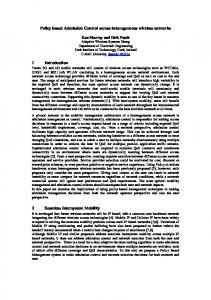
For the forthcoming stability analysis we determine for which control parameters the linear subsystem Gz is stable. The poles of (11) are stable for the area depicted in Figure 5 for the normalized parameters K/σ and h/Ti .

2

a2

1

0

−1

−2 −3

−2

−1

0 a

1

2

3

1

60 40

h/Ti

20 0

−20 −40 −60 −0.4

−0.2

0

0.2

0.4

K/σ

Fig. 5. (Upper:) The internal of the triangle corresponds to the stability area for the characteristic polynomial z · (z 2 + a1 z + a2 ) of Gz . (Lower:) Corresponding stabilizing control parameters {K/σ, h/Ti }.

C. Stability analysis for discrete-time nonlinear system To determine the stability for the nonlinear system in (11) we can use the Tsypkin criterion or the Jury-Lee criterion which are the discrete-time counterparts of the Popov criterion for continuous time systems [16]. Sufficient conditions for stability are that G z has all its poles within the unit circle |z| < 1 and that there exists a (positive) constant η such that 1 ≥ 0 for z = eiω , ω ≥ 0 (12) k where the nonlinearity φ belongs to the cone [0, k = 1]. In the upper left plot of Figure 6 we have the stability triangle for the characteristic polynomial of Eq.(2). By choosing coefficients for the characteristic polynomial (2) in the upper left triangle (A1) we will get controller parameters {K, T i } which also will give a stable transfer function G z . The corresponding poles are plotted in the lower diagram of Figure 6. Figure 6 shows a graphical representation of the Tsypkin condition (12) for this set of control parameters. The dashed non-intersecting line in Figure 6 corresponds to the existence of a positive parameter η satisfying Eq.(12). Thus, absolute stability for the nonlinear system also is guaranteed for this choice of parameters. Remark: The Tsypkin criterion guarantees stability for any cone bounded nonlinearity in [0, 1] and we can thus expect to have some robustness in addition to stability in our case. Re[(1 + η(1 − z −1 ))Gz (z)] +

V. E XPERIMENTS The admission control mechanism was implemented in the Apache web server. Apache is made up of a core package and several modules that handle different operations, such as Common Gateway Interface (CGI) execution, logging, caching etc. A new module was created that contains the admission control mechanisms. The new module was then hooked into the core of Apache, so that it was called every time a request was made to the web server. The module could then either reject or admit the request according to the control mechanism. The admission control mechanism was written in C and tested on a Windows platform. We tested the system by running tests on it and collecting performance

Tsypkin plot

2

Stability region of characteristic polynomial z +a1z+a2

10

2

1

a2

A1 0 5

−2 −6

−4

−2

0 a

2

4

6

1

pole location

Re(1−1/z)G(z)

−1

0

0.5

0

−0.5 −5 −5

−3

−2

−1

0

1

2

3

0

5

10

Re(G(z))

Fig. 6. (Upper left:) The large triangle is the stability area a linear model would predict. However, from this parameter set, nonlinear analysis guarantees only stability for parameters {a1 , a2 } in the upper left triangle (A1 ,
∗
). (Lower left:) Pole location corresponding to {a , a }∈ A1. (Right:) Set of Tsypkin plots which all satisfy 1 2 the frequency condition (12) for Gz = Gz (K, Ti ), where (K, Ti ) correspond to pole locations to the left

metrics such as the server utilization distribution and step responses. We also compared the measurements with simulations. The queueing model was represented by a discrete-event simulation program implemented in C, and the control theoretic models were implemented with the Matlab Simulink package. The traffic generators in the discrete-time model were built as Matlab programs. They generate arrivals and departures according to the given statistical distributions. A. Setup Our measurements used one server computer and one computer representing the clients connected through a 100 Mbits/s Ethernet switch. The server was a PC Pentium III 1700 MHz with 512 MB RAM running Windows 2000 as operating system. The computer representing the clients was a PC Pentium II 400 MHz with 256 MB RAM running RedHat Linux 7.3. Apache 2.0.45 was installed in the server. We used the default configuration of Apache. The client computer was installed with an HTTP load generator, which was a modified version of S-Client [17]. We modified the S-Client code to use Poissonian arrivals instead of the original deterministic ones. The client program was programmed to request dynamically generated HTML files from the server. The CGI script was written in Perl. It generates a number of random numbers, adds them together and returns the summation. The average request rate was set to 100 requests per second in all experiments except for the measurements in Figure 7. In all experiments, the control interval was set to one second. B. Validation of the Model We have validated that the open system, that is without control feedback, is accurate in terms of average server utilization. The average server utilization for varying arrival rates are shown in Figure 7. For a single-server queue, the server utilization is proportional to the arrival rate, and the slope of the server utilization curve is given by the average service time. The measurements in Figure 7 gives an estimation of the average service time in the web server, 1/µ=0.0225.

100

Server utilization

80

60

40

20

0 0

5

10

15

20

25

30

35

40

requests/second

Fig. 7.

Average server utilization for the open system.

C. Controller parameters Control parameters for the PI-controller are chosen from the stability area A1 in Figure 6. In the simulations and experiments below we use {K, T i }={20, 2.8}. The parameter setting is also compared to {K, T i }={20, 0.1}, found outside the stability area. D. Performance metrics An admission control mechanism has two control objectives. First, it should keep the control variable at a reference value, i.e. the error, e = y ref −y, should be as small as possible. Second, it should react rapidly to changes in the system, i.e. the so-called settling time should be short. Therefore, we test the mechanism in two ways. First, we show the steadystate distribution of the control variable, by plottting the estimated distribution function. The distribution function is estimated from measurements during 1000 seconds with the specific parameter setting. Second, we plot the step response during 60 seconds when starting with an empty system. E. Distribution function Figure 8 shows the estimated distribution function for the PI-controller. Both good and bad parameter settings were used. An ideal admission control mechanism would show a distribution function that is zero until the wanted load, and is one thereafter. In this case, the load was kept at 0.8, and the parameter setting, {K, Ti}={20, 2.8}, chosen from results in a controller that behaves very well in this sense. The parameter setting, {K, T i }={20, 0.1}, as can be seen, perform worse. Also, as comparison, results from simulations of the M/D/1 system and the M/M/1 system are given in Figure 8, when using {K, T i}={20, 2.8}. F. Step response Figure 9 shows the behaviour of the web server during the transient period. The measurements were made on an empty system that was exposed to 100 requests per second. The good parameter setting, {K, T i}={20, 2.8}, exhibits a short settling time with a relatively steady server utilization. The bad parameter setting, {K, T i}={20, 0.1} has its poles outside the unit circle and behaves badly, the load oscillates and is never stable. Comparisons to M/D/1 and M/M/1 simulations, also in Figure 9, show that the model is accurate. VI. D ISCUSSION The analysis in Section IV-C gives sufficient conditions and a region for control parameters which guarantee stability of the nonlinear closed loop as well as for the simplified linear model. We are of course not restricted to choose parameters from only this region as the main objective is that the nonlinear system should be stable. However, we can conclude that

1 (20, 2.8) (20, 0.1) 0.8

P(utilisation