Adsorptive characterization of porous solids

- Supplementary Information -

Adsorptive characterization of porous solids: Error analysis guides the way Martijn F. De Lange[1,2], Thijs J.H. Vlugt[2], Jorge Gascon[1] and Freek Kapteijn[1] [1]

Catalysis Engineering, Chemical Engineering Department, Delft University of Technology,

Julianalaan 136, 2628 BL Delft, Netherlands [2]

Process & Energy Laboratory, Delft University of Technology, Leeghwaterstraat 39, 2628

CB Delft, The Netherlands

1

LIST OF SYMBOLS Latin Symbol Description

Unit

Acs C c D E F

Cross-sectional area Dimensionless BET parameter Dimensionless ratio of Kelvin and pore radius Diameter Adsorption energy F-test statistic

m2 m kJ mol-1 -

I K

Intercept Langmuir adsorption equilibrium constant

g mlSTP-1 bar-1

MN2

Molar mass of nitrogen

g mol-1

N n

Number Amount

mol

NA p p

Avogadro's constant Pressure Number of parameters to be estimated

mol-1 bar -

p/po

Relative pressure

-

q R r R(n) R2 res S

Adsorbed amount Universal gas constant Radius Pore aspect ratio Coefficient of determination Residual Specific surface area

mlSTP g-1 J mol-1 K-1 m -

s

Slope

g mlSTP-1

SSE

Error sum of squares

[varies]

SSL SSR T t t V Vp

Lack-of fit sum of squares Sum of squared residuals Temperature Thickness of adsorbed layer Student t-distribution Volume Specific pore volume

[varies] [varies] K m m3 ml g-1

Vl w Z Greek Symbol α α

Liquid molar volume Weight Compressibility factor

m3 mol-1 g -

Description Linear correction factor Confidence level (in Student’s

(a)

m2 g-1

Unit bar-1 2

β ζ ρ

t-distribution) Dimensionless ratio (see Eq. S-15.3) Parameter (either Vp or SBET) Density

σ σ2

Standard deviation or uncertainty Variance

(a,b)

σt ω

Surface tension Statistical weight

dyn cm-1 -

[varies] g ml -1 (c)

Subscript ads

Adsorbed

BET

Brunauer, Emmett and Teller (method)

cell

Sample cell

cold

Cold fraction of the sample cell

d

Dose

D.O.F. Degree(s) of freedom dosed

Dosed

gas

Present in the gas phase

K

Kelvin

l

Linear

m

Monolayer

man

Manifold

nbp

Normal boiling point

p

Pore

res

Residual(s)

sample Sample of (porous) material sat

At saturation

STP

Standard temperature and pressure (d)

warm

Warm fraction of the sample cell

Superscript Liquid phase liq S

Studentized

vap

Vapour phase

Notes: (a)

Same units as the property it is related to

(b)

Standard deviation if based solely on measured values, else uncertainty

(c)

Squared units of the property it is related to

(d)

273.15 K and 1 bar 3

SUPPLEMENTARY MATERIAL

This supplementary information file contains all relevant experimental and theoretical details, additional adsorption measurements and calculations, divided over the following subsections: S-1: Sample mass and cell volume for repeated measurements................................................ 5 S-2: Error propagation in nitrogen physisorption measurements............................................... 5 S-3: Calculation of BJH-pore size distribution and uncertainty therein .................................. 10 S-4: Calculating the confidence interval for BET parameters determined with the linear method ...................................................................................................................................... 13 S-5: Calculated confidence intervals for nitrogen adsorption isotherms ................................. 15 S-6: Breakdown of uncertainties ............................................................................................. 16 S-7: Influence of experimental variables on uncertainty in adsorbed amount and pore volume – theoretical study .................................................................................................................... 24 S-8: Influence of experimental variables on measurements using γ-alumina(2) – experimental study ......................................................................................................................................... 30 S-9: Influence of dosing on uncertainty of nitrogen adsorption isotherms .............................. 42 S-10: Detailed BET area and confidence interval using the linear method ............................ 49 S-11: BET – Comparison of (weighted) direct and linear fitting ............................................. 57 S-12: Residuals ......................................................................................................................... 61 S-13: The two-point BET method ............................................................................................ 65 S-14: Studentized residual plots and predictions for γ-alumina and MIL-101(Cr).................. 66 S-15: Variation of pore volume and BET surface area obtained from different measurements of the same material sample ..................................................................................................... 73 S-16: Weights used for linearization ........................................................................................ 78 S-17: Weighted direct method.................................................................................................. 78 S-18: Lack-of-fit test for repeated isotherm measurements ..................................................... 79 S-19: Recalculating BET and pore volume for MIL-101(Cr) retrieved from various literature sources ...................................................................................................................................... 84 S-20: BJH pore-size distributions based on adsorption branch................................................ 87

4

S-1: Sample mass and cell volume for repeated measurements Sample masses of materials used in the adsorptive investigations and sample cell volumes determined are given in Table S 1. Table S 1: Samples masses and cell volumes used in nitrogen adsorption measurements. Manifold volume is 24.3 ml. Material wsample / g MIL-101(Cr) 0.12 UiO-66 0.13 Sigma-1 0.15 γ-alumina 0.18 NORIT RB2 0.20

Vcell / ml 10.5 11.0 11.1 10.8 10.7

S-2: Error propagation in nitrogen physisorption measurements The variance in a measured nitrogen isotherm is calculated using propagation of uncertainty (see, e.g. Taylor [1]): 2

 y  2      xi  xi  2 y

(S-2.1)

Here y is a variable calculated from i measured variables xi and σy is the uncertainty in this variable y, clearly a function of the uncertainties in xi, σxi. Applying Eq. (S-2.1) consecutively on all calculated variables, will ultimately lead to the uncertainty the adsorbed amount as function of relative pressure. An adsorption measurement in general starts with the determination of the volume of the sample cell, Vcell, which is connected to the dosing manifold. This dosing manifold is a vessel of which the volume, Vman, is accurately determined by the manufacturer. The determination of Vcell is started by pressurizing the manifold with helium and then opening the connection 5

between manifold and sample cell, which is at or near vacuum before connection to manifold is opened. The cell volume can then be calculated via:

Vcell

0  pman  p1man   1  Vman 0  pcell  pcell 

(S-2.2)

Here, pman is the manifold pressure, pcell is the cell pressure, and indices 1 and 0 correspond to after and before opening the connection between manifold and cell, respectively. Error propagation dictates thus that the variance in the cell volume is: 2

 V2

cell

2 2  0  0    pman  p1man  2 pman  p1man 1 2 2   Vman   2 p   V  1  2 p    p1  p 0   Vman (S-2.3) 0   p1  p 0 2 man  cell   pcell  pcell   cell cell  cell 

Here σp is the uncertainty in any of the measured pressures, irrespective of which volume it belongs to. As nitrogen adsorption measurements are performed at the normal boiling point of nitrogen (77.4 K), a part of the sample cell volume will be cooled to this temperature, called the cold volume, Vcold, and a part of this volume will remain at room temperature, Vwarm. To determine both, the sample cell is now pressurized with helium, before the cooling is applied. After cooling, the pressure in the sample cell will have decreased. From this decrease, the warm part of the cell volume, Vwarm, can be quantified by:

Vwarm

0  pcell Twarm  1  p Tcold   cell Twarm   1 T cold 

   Vcell   

(S-2.4)

Here Twarm is the temperature of the manifold, and Tcold is the temperature of liquid nitrogen. Hereby it is assumed that the thermal conditions are the same under helium and nitrogen and that these don’t change during adsorption measurements. 6

The variance in the warm fraction of the cell volume can be calculated via: 2

 V2

warm

0 2  pcell    2   2   1 0 1    pcell   2  Tcold  pcell  pcell  1 2   Vcell  p   Vcell   p   1 Vcell   T2warm   1  T  T p T  T   1  warm   cell  warm cold    pcell 1  warm   Tcold    Tcold      (S-

0 1  Twarm  pcell  pcell  V   2   1 2 cell   Tcold  pcell Twarm  Tcold   2

0  pcell Twarm  1  p Tcold   cell T  warm  1 T cold 

2

    V2  cell  

2.5) Here σTwarm is the uncertainty in the measured temperature in the manifold, and σTcold is uncertainty in the liquid nitrogen temperature. The latter is caused by minor fluctuations in ambient pressure of the surrounding atmosphere as measured periodically by the machine and thus the uncertainty in Tcold is back-calculated via the Antoine equation. In practice this uncertainty is rather similar to σTwarm. The cold volume and variance therein are easily found via subtraction:

Vcold  Vcell  Vwarm

(S-2.6)

V2  V2  V2

(S-2.7)

cold

cell

warm

After these volume determinations, the actual measurement can be commenced. This is effectively commenced by evacuating the sample cell, to remove all the helium present and supplying a given pressure of nitrogen to the manifold. The connection between sample and manifold is opened and the material under investigation will start to adsorb nitrogen. After equilibration, in this analysis it is tacitly assumed that thermodynamic equilibrium is reached, the amount adsorbed for the first measured point is calculated as the difference of the total 7

amount dosed and the amount of nitrogen pressure present in the gas-phase in the sample cell. From the second measured point and onwards this difference is augmented with the amount adsorbed for the previous point(s):

nads  i   ndosed  i   ngas  i   nads  i 1

(S-2.8)

Here nads is the amount adsorbed, ndosed the amount dosed from the manifold and ngas is the amount present in the gas phase, all in moles. The amount present in the gas phase can be calculated via:  V Vcold i  warm  ngas  i   pcell i  RTwarm Z  pcell  RTcold 

   

(S-2.9)

Here Z is the compressibility factor, a correction for non-ideality, defined as: i Z  1   Tcold  pcell

(S-2.10)

Here α is the linear correction factor. The amount dosed can be calculated via: 0 (i )  p1man (i )  ndosed (i )   pman

Vman V  pman (i ) man RTwarm RTwarm

(S-2.11)

For now it is tacitly assumed that a single dose will be sufficient to measure a point on the isotherm. In Appendix S-4 the effect of not adhering to this assumption on uncertainty is shown. The variance in ngas, ndosed and nads respectively can now be calculated:

8

 i pcell  T  Vcold V Vcold 2  ngas  i    warm   i  RTwarm RT Z  p  i cold cell RTcold Z  pcell  



2

i   pi V  pcell   cell warm2   T2warm   i    Z  pcell  RTcold  R Twarm   

2

   V2cold  

2

2  i   2   pcell   2   Vwarm p 2    RTwarm   (S-2.12) 2 i   pcell Vcold   T2  2 i  Z  pcell  R Tcold   cold  



2



2 ndosed

 n2

ads

2 2  p (i)  2  Vman   pman (i )  2 2 man V   Twarm   i     2 p     Vm 2 man   RTwarm   RTwarm   R Twarm  

 i    n2  i    n2  i    n2  i  1 gas

dosed

ads

(S-2.13)

(S-2.14)

Clearly, the variance is of a cumulative nature. Each point is determined in parts by what has been measured the point before, hence propagating the uncertainty of each point into the next. The equipment used actually does not report the amount dosed, so to be able to calculate the uncertainty in the amount dosed, essential in this error analysis, a back-calculation of this quantity is required before proceeding, via:

ndosed  i   nads  i   nads  i 1  ngas  i   ngas  i 1

(S-2.15)

Often the loading is expressed in either mmol g-1 or mlSTP g-1. Hence the uncertainty in sample mass has to be taken account. For the former case:

q i  

nads  i 

(S-2.16)

wsample

Here wsample is the sample mass used. The variance is thus: 2

2  n i   1  2 ads    2  q i      w2sample  i  nads    2 w  w   sample   sample  

(S-2.17)

9

Note that the variance in sample mass is often twice that based on the accuracy of the balance used. This because the sample mass is often determined as difference of the sample holder empty and filled. The uncertainty can obviously be reported in mlSTP g-1 as well, just by multiplication with the molar volume at standard temperature and pressure (1 bar and 0o C). Lastly, one could also introduce the uncertainty in the relative pressure but this turns out to be negligible. Of the measured quantities pressure, temperature and mass, the standard deviation provided by the equipment’s suppliers have been used. The 95% confidence interval is ±1.96·σq. S-3: Calculation of BJH-pore size distribution and uncertainty therein First step in the determination of a BJH pore size distribution is the calculation of pore size, rp, for each relative pressure. This pore size is the sum of the statistical thickness, t, herein calculated using the Harkins-Jura equation [2, 3], and inner capillary radius, rk, determined with the Kelvin equation: rp  r K t

(S-3.1)

    13.99  t     po   log10    0.034   p   

(S-3.2)

r K

2 tVl p  RT ln  o   p

(S-3.3)

Here σt represents surface tension and Vl is the liquid molar volume of nitrogen. According to the propagation of errors [1], the uncertainty in the pore radius can be calculated as function of uncertainty in relative pressure, using: 10

2

        13.99   ln 10    2 2  t2   0.5  p     p  ln o  po       p   0.034  ln  po   0.034 ln 10      p      ln 10        

(S-3.4)

2

 r2

K

      2 2 tVl   p 2    po    p   po  RT ln  p    p        o   

(S-3.5)

 r2   r2   t2 p

(S-3.6)

K

The uncertainty in relative pressure is taken from the uncertainty analysis results of adsorption isotherms, (see Figure 2), wherein it was not depicted because of the small values thereof. Next step is to determine the dimensionless factors for each interval between two measured points, Ri and ci, respectively, via:  rp  R   rK  t 

c

2

(S-3.7)

rK rp

(S-3.8)

Uncertainty herein can be calculated according to: 2

2

  2  2rp2  2rp  R2        r2K   2t   r  t 2  rp   r  t 3   K   K 





(S-3.9)

11

2

2

r  1    K2   r2p     r2K r  r   p   p 2 c

 

(S-3.10)

Uncertainty in the average Kelvin- or pore radius belonging to two adjacent data points and the difference in statistical thickness can be calculated using respectively:



2 r

 

2 r

(i )   r2 (i  1) 

(S-3.11)

22

and

 2t   t2 (i )   t2 (i  1)

(S-3.12)

The pore volume distribution can be calculated by applying following equation starting from a measured point at saturation recursively either down the ad- or desorption branch: n 1    vap. Vp  n   R  n   q  n  STP t n c j S p, j       liq .    nbp j 1  

(S-3.13)

Assuming a cylindrical pore geometry, the specific surface area of each pore increment, Sp,j, can be calculated using:

S p n 

2V p  n 

(S-3.14)

rp

For the pore volume thus, one can derive for the variance: 2

2

vap . vap . n 1   STP  2   STP    n    liq. q  n   t  n   c j S p , j   R  n    liq. R  n    2q  n      j 1  nbp   nbp  (S-3.15) 2   n n 1 1   2   R  n   c j S p , j   2t  n    R  n  t  n    S p2, j c2j  c 2j  S2p , j j 1 j 1   2 V pore





12

Here the variance of the differential volume adsorbed is given by

 2q   q2 (i )   q2 (i  1)

(S-3.16)

The variance in q (in mlSTP g-1) was calculated previously, and depicted in Figure 2. Lastly, the variance in surface area of each pore can be calculated via: 2

 2V  n   2  s2p  n    p 2   r2p    r  r p    p

2

 2   Vp 

(S-3.17)

Often the pore size distribution is visualized with ΔVp/ΔDp. The variance therein can be calculated using:



2 V p D p

 1   D p 

2

2

 2  V p  2    V p   2   Dp D  p   

(S-3.18)

Here the variance in ΔVp and ΔDp can be calculated in the same manner as for Δq (see Eq. S3.16). S-4: Calculating the confidence interval for BET parameters determined with the linear method Recall that the monolayer capacity is calculated from:  1  qm   , I S 

I s C    I 

(S-4.1)

Clearly, the uncertainty in the monolayer capacity and C parameter are a function of both the uncertainty in intercept and slope. As the intercept and slope are determined via least-squares fitting, one can write for the uncertainty in these parameters [1]: 13

I   y

xi2 i 

(S-4.2)

s   y

N 

(S-4.3)

Here xi are the relative pressure of each data point, yi is the left-hand side of Eq. 5 for that same data point and N is the total number of data points included in fitting. As there are two fitted parameters, the degrees of freedom is the total number of data points, N, decreased by two. The uncertainty, σy, in predicted values and the denominator in above equations, and Δ are given, respectively by [1]:

(S-4.4)

    N  x    xi  i  i 

2

2 i

(S-4.5)

As slope and intercept are determined from the same fit, the uncertainties are not expected to be devoid of correlation. Consequence is that in calculation of the uncertainties in BET area and C parameter, the covariance of I and s should be included: 2

2

 B   B   B    B       I2     s2  2      I , s  I   s   I   s  2 B

(S-4.6)

Here B is either the monolayer capacity or the BET C parameter, and σI,S is the covariance of the regression coefficients, given by: 14

 I ,s  

2 y

x

i

(S-4.7)

i



Finally, the uncertainties in the BET parameters can be calculated: 2

 q2

m

 1  2   I ,s   I2   s2   2 4   I  s   I s     2

(S-4.8)

2

s  s  1    2   I2     s2  2 3  I , s I I  I 2 C

(S-4.9)

Confidence interval is now determined using:

Bt



1 , DOF 2

B

(S-4.10)

Here t stands for Student’s t-distribution, α is the confidence level (0.05 for a 95% confidence interval) and DOF stands for the number of degrees of freedom. Again, B stands for either qm or C. Obviously, for the uncertainty in the BET surface area, one can write:

S

BET

  qm

vap .  STP N A ACS

M N2

(S-4.11)

S-5: Calculated confidence intervals for nitrogen adsorption isotherms Figure S 1 shows the confidence interval in the adsorption isotherm calculated using the propagation of uncertainties for the third isotherm measurement of each material.

15

Figure S 1: Absolute error in measured adsorbed N2 amount as function of relative pressure for both ad- and desorption branch of the materials under investigation. For each material the third of three isotherm measurements is depicted. S-6: Breakdown of uncertainties It is insightful to investigate the different contributions to the 95% confidence intervals depicted in Figure 2, especially when one aims to improve the accuracy of adsorption measurements. Starting point is the variance in the isotherm, as given by Eq. S-2.17, from which the fractional contributions to the variance in the adsorption measurements can be calculated. For all measurements the first term in Eq. S-2.17 was found very dominant in the total variance: 2

 n i   1  2  ads     w2 2 sample    nads  i   w  sample    wsample     q2  i   q2  i  2

(S-6.1) 16

So, the variance in amount adsorbed, nads, has a significantly higher contribution to the overall uncertainty than the variance in weighing of the investigated samples. Consequently one can rightfully conclude that sample weighing on a balance with an accuracy of ± 0.1 mg is more than sufficient. Unless of course a much smaller sample is used than in this work (0.1-0.2 g). In that case the right hand side term in Eq. S-6.1 is no longer negligible. This situation however is to be avoided and not taken further into account. The variance in amount adsorbed nads(i) has three contributions per measured point (see Eq. S-2.14) related to the uncertainty in determination of the amount present in the gas phase, ngas(i), the amount dosed, ndosed(i), and the amount adsorbed for the previous measured point, nads(i-1). To conveniently compare the different contributions to the variance in nads(i), the following dimensionless fractions have been defined :

 gas  i  

i   i 

 n2

gas

2 nads

 n2  dosed  i   2 n

dosed

ads

i  i 

 n2  i  1  ads  i  1   1   dosed  i    gas  i   n2  i  ads

(S-6.2)

(S-6.3)

(S-6.4)

ads

These fractions are calculated for the third isotherm measurement of each of the materials, both under simplifying assumption of a single dose per measured point as well as for the most stringently incorporated dosing threshold in this work. Results are depicted in Figure S 2.

17

a)

b)

18

d)

e)

Figure S 2: Fractional contributions to the variance in the amount adsorbed, κ, calculated according to Eq. S-6.2 - S-6.4 for MIL-101(Cr)(a), UiO-66(b), Norit RB2(c), γ-alumina(d) and Sigma-1(e), assuming either a single dose per measured point (left), or using the most stringent dosing threshold (7.10-3 Pa) for dosing (right), as function of the point measured. Dashed line indicates the transition from ad- to desorption.

Clearly for all materials the largest contribution stems from that of the previous data point κads(i-1), which is not surprising because of the cumulative nature of the propagation of uncertainties for adsorption. Furthermore, for low relative pressure, (p/po) < 0.10 - 0.15, (corresponding to the first 10-20 data points, see Figure S 3), κdosed is larger than κgas. At higher relative pressure this relative order is reversed and the gas-phase contribution becomes 19

more dominant. This is easily rationalized, as the gas-phase variance is strongly increasing with pressure (see Eq. S-2.12), whereas the variance in the amount dosed is related to the pressure difference over the manifold Δpman (see Eq. S-2.13 and S-9.5), which is dependent on the adsorption behaviour of the material under investigation (nads(i) - nads(i-1)), which thus does not show a continuous increase as function of pressure. The transition point is shifted to higher pressures for more mesoporous materials (see Figure S 2), as for these materials adsorption uptake continues up to higher relative pressures. Also, if one does not assume a single dose per measured point (see S-9, S.I), this transition pressure is shifted to higher values (see Figure S 2).

Figure S 3: Relative pressure belonging to each measured point. Dashed line indicates the transition from ad- to desorption. Taken from the third measurement of γ-alumina, but the distribution of data points over the relative pressure range is very similar for all conducted measurements. 20

From this analysis, it can be deduced that the variance in amount present in the gas-phase, σ2ngas, should be decreased if one wants to significantly decrease the uncertainty in the full adsorption measurement. If one is particularly interested in the low relative pressure regime, however, the variance in amount dosed should be targeted. The former is investigated further first. The variance in the amount present in the gas-phase, dominantly present in the uncertainty for (p/po) > 0.10 - 0.15, is determined from five separate terms (see Eq. S-2.12), for which the fractional contributions can be calculated:

 i pcell  T  Vcold Vcold  Vwarm    RTwarm RT Z  pi  i cold cell RTcold Z  pcell    gas 1  i    n2gas  i 



2



  2 p 2   

(S-6.5)

2

i  pcell  2   V RTwarm  warm   gas 2  i    n2gas  i 

(S-6.6)

2

 pi V   cell warm2   T2warm  R T   warm   gas 3  i     n2gas  i 

i  pcell  i  Z  pcell  RTcold   gas  4  i    n2gas  i 

(S-6.7)

2

   V2cold  

(S-6.8)

2

i   pcell Vcold    T2 2 i  Z  pcell  R Tcold   cold   gas 5  i     n2gas  i 

(S-6.9)

21

These fr fractions callculated forr all the perrformed meaasurements are depicteed in Figuree S 4 for MIL-1001(Cr) and UiO-66. U Bo oth from Eqq. S-6.5-9 and a Figure S 4 it can bbe seen that the gasphase vvariance contributions are not saample speciific and thu us not deppicted for th he other materialls.

a)

b)

butions to tthe variancee in gas-phaase, as calcuulated from m Eqs. SFigure S 4: Fractional contrib 6.5 - S-66.9, for MIL L-101(Cr)(a a) and UiO--66(b).

d Clearly,, at low relaative pressure ((p/po) < 0.05-0.06)) the first teerm (Eq. S-66.5) is the dominant contribuution to the variance in n amount prresent in th he gas-phasee, above thiis the fourth h term is largest (Eq. S-6.8)). Recall ho owever thatt for p/po < 0.10 - 0.1 15 the variaance in the amount dosed iis larger thhan variancce in the amount gaas phase, and a that thhus decreassing the contribuution of Eq.. S-6.5 is off little use. So, for meaasurements that includee p/po > 0.10 - 0.15, the variance in thhe cold parrt of the ccell volumee, σ2Vcold, should s be ddecreased to t make measureements morre accurate. For meeasurementss where thee region (p/ p/po) < 0.10 0 - 0.15 is essential, one should d aim at decreasiing the varriance in th he amount dosed (Eq q. S-2.13 or o S-9.5 if single dose is not 22

assumed). For all measurements under investigation, the dominant term for all measurements under investigation is the first (for both Eq. S-2.13 and S-9.5), indicating that accurate pressure measurement is key for low relative pressures. Returning to the case where the region (p/po) > 0.10 - 0.15 is of interest, the variance in the cold part of the cell volume should be reduced. As this is a calculated property, it is interesting to find out which measurement should be conducted more accurately. To do so the uncertainty in cold volume is broken down into two contributions (see Eq. S-2.17), of which the relative importance is calculated, based on available measurement data:

 V2  V2

 0.658  0.006

(S-6.10)

 V2  V2

 0.342  0.006

(S-6.11)

warm

cold

cell

cold

This indicates that both volumes contribute to the variance of the cold volume, of which the warm volume is more important. If in turn the variance in the warm volume (Eq. S-2.5) is investigated, it can be found, for the different measurements, that the fifth term is dominant: 0  pcell Twarm  1   pcell Tcold  1  Twarm  Tcold 

 V2

2

    V2  cell    0.973  0.004

(S-6.12)

warm

Clearly, decreasing variance in the cell volume is crucial to increase the accuracy of the adsorption measurement, when (p/po) > 0.1. From Eq. S-2.3 and data from the different measurements the relative contributions to this variance from the pressure sensor and of the manifold volume can be found: 23

2   2   0 1   pman  pman 1    Vman   2 p2  2   p1  p 0 Vman    1 0 cell    pcell  pcell   cell      0.69  0.01

 V2

(S-6.13)

cell

2

0  pman  p1man  2  1   Vman 0  pcell  pcell   0.31  0.01 2

V

(S-6.14)

cell

This indicates that a more accurate calibration of the manifold volume would help decreasing the uncertainty in adsorption experiments, as σ2Vman would be decreased. But, as was also shown for low pressure measurements, it is best to decrease the accuracy of the used pressure sensor. Lastly, as the pressure difference in the cell (pocell - p1cell) is a function of the manifold pressure difference (poman - p1man) and the ratio (Vman/Vcell) (see Eq. S-2.2), one could optimize this ratio also to decrease the uncertainty. Result of this analysis is that this ratio is optimally between 2 and 3 (see S-7, S.I.). S-7: Influence of experimental variables on uncertainty in adsorbed amount and pore volume – theoretical study The effect of the sample amount used during a measurement and the ratio of manifold and cell volume, (Vman/Vcell) on error propagation is investigated by calculating the uncertainty in the pore volume for a Langmuir isotherm, rewritten to incorporate relative pressure: p   K p0 q  qm   1 K p  p0 p0 

     

(S-7.6)

Results are depicted in Figure S 5.

24

Figure S 5: 95% confidence interval for tthe calculatted pore vollume at (p/ppo) = 0.9 as function of sampple mass useed for a Lan ngmuir isottherm (qm = 500 mlSTP g-1, K = 100 bar-1) for different values oof (Vman/Vcelll). Pore vollume and 5% % thereof (b both in mlSTTP g-1) are de depicted as solid s and dashed line, respectively. In nsert showss the same 95% confiidence interrval as fun nction of (Vman/V Vccell) for a sam mple mass of o 0.2 g.

The effe fect of sampple mass is clear. If leess than 0.0 05 gram is used, u the un uncertainty becomes b prohibittively high. The more mass m is useed the betterr, but the deecrease in uuncertainty becomes b less witth increasinng mass. Th his observattion is expllained by Eq. E S-2.17. The uncerrtainty is roughlyy a function of wSample-1, because thhe amount adsorbed a nadds is a linearr function of o wSample as well.. For low vaalues of (V Vman hus large ceell volume, the uncertai ainty is very y high as m /Vcell), th well. Thhis is attribuuted to two reasons. Fiirstly, a larg ge cell volum me increasees uncertain nty in the amountss adsorbed and presentt in the gas pphase (Eq.ss S-2.12, S-2.14). Secoondly, uncerrtainty in the cell volume is increased severely. Iff the cell volume v is much m largerr than the manifold m 25

volume, there is hardly any pressure difference in the cell when the cell volume is calculated by expanding helium (Eq. S-2.2). This small pressure difference increases the uncertainty in the cell volume substantially (Eq. S-2.3). A value for (Vman/Vcell) larger than 3 would increasingly lead to a larger uncertainty. So, to decrease the uncertainty, the sample cell would ideally be about half of the manifold volume (2 ≤ (Vman/Vcell) ≤ 3). Note that for these calculations, the single dose assumption was used. Uncertainties might become higher when using a dosing threshold, depending on material properties. Above results are for one single Langmuir isotherm. The influence of both the equilibrium constant, K, and monolayer capacity, qm, on (relative) uncertainty of the pore volume (e.g. pore volume filling of zeolites can described with a Langmuir-type isotherm) is given in Figure S 6.

26

Rel. 95% conf. Int. / -

a)

qm / mlSTP g-1

K / bar-1

Rel. 95% conf. Int. / -

b)

qm / mlSTP g-1

K / bar-1

Rel. 95% conf. Int. / -

c)

qm / mlSTP g-1

K / bar-1

Figure S 6: Relative confidence interval in pore volume as function of Langmuir parameters monolayer capacity, qm, and equilibrium constant, K, for a sample mass of 0.05 g (a), a mass of 0.5 g (b) and both a mass of 0.5 g and a dosing threshold, Δpmax, of 0.07 bar (c). For all calculations, the ratio (Vman/Vcell) was set to 2.

27

The choice was made to depict the uncertainty normalized by the pore volume, as the pore volume is a function of both K and qm. Clearly, for low values of K and qm, the relative uncertainty is very high. Up to 50% for 0.05 g of material (Figure S 6a). This is because a material with low values of both parameters hardly adsorbs any nitrogen (see Figure S 7).

Figure S 7: Langmuir isotherms, normalized by monolayer capacity, qm, for different values of equilibrium constant, K, as function of relative pressure.

Increasing the amount of material to 0.5 g significantly decreases the relative uncertainty (Figure S 6b), not changing the shape of the surface. Again, this is under the assumption of single dosage. Therefore, for 0.5 g, the relative uncertainty has been recalculated, now encompassing a dosing threshold, Δpmax of 0.07 bar (see Figure S 6c). Again at low K and qm, a high relative uncertainty is seen. A difference, with the previous case is however, the 28

dependency of the uncertainty on K. The uncertainty is higher than under the single dose assumption, at high values of the equilibrium constant. This is due to the fact that a high equilibrium constant mimics the properties of a microporous material (See Figure S 7) and thus requires a significant number of doses for the first measured adsorption point. For the case of 0.05 g sample mass, the difference in uncertainty between single dosing and using a dosing threshold is more or less negligible and thus the threshold case is therefore not depicted. Lastly, in Figure S 8, relative confidence interval in pore volume calculated at (p/po) = 0.9 is given as function of qsat wsample, for easy estimation of uncertainties of performed measurements.

29

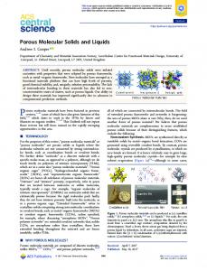
Figure S 8: Relative 95% confidence interval of pore volume Vp depicted as function of total amount adsorbed (qsat wsample). Calculated using the single dose assumption. S-8: Influence of experimental variables on measurements using γ-alumina(2) – experimental study In this work the sample mass and cell volume were deliberately kept constant for the three repeated consecutive measurements (see Figure 2) to investigate the reproducibility of this measurement procedure. It is as important, however, to investigate the effect of sample mass and cell volume on adsorption measurements of one material. A notably different sample of γalumina (000-3p, Akzo Nobel), denoted as γ-alumina(2), was used for this purpose. This because γ-alumina(2) has a larger desorption hysteresis compared to the γ-alumina used in the rest of this work (CK-300) and the variation of cell volume has a notable effect especially on desorption, as will be shown. To reduce effects of possible sample inhomogeneity, the first conducted measurement of each of the five different cells contained the highest sample mass (~ 0.14 g). For the second and third measurements, from this mass ~0.05 g was removed from the previously measured sample. Sample holders with different volumes (four types were available), the smallest one was used also with a supplemented a glass rod to reduce the sample holder’s volume further. This yielded the five cell volumes and different sample masses for the three subsequent measurements in each cell as depicted in Figure S 9.

30

Meas. 3

Meas. 2

Meas. 1

Figure S 9: Sample mass and cell volume calculated during measurements for the three separate measurements (about 0.14, 0.09 and 0.05 g for the 1st, 2nd and 3rd measurement, respectively) and the five different cells used in this study. In the background an image of the different sample cells and the glass filler rod (used in Cell 1()) are shown. Dashed lines connect the cell volume curve with the image. Manifold volume is 24.3 ml.

Measured adsorption isotherms and calculated confidence intervals are depicted in Figure S 10.

31

a)

b)

c)

d)

e)

Figure S 10: Repeated isotherms measurements for -alumina(2) and confidence intervals calculated using error propagation for Cell 1 (a), Cell 2 (b), Cell 3 (c), Cell 4 (d) and Cell 5 (e). First(), second() and third() measurement depicted with closed symbols, 32

confidence intervals given with lines and open symbols. Measurement conditions can be found in Figure S 9. As was expected (see Figure S 5), decreasing sample mass and increasing cell volume both enlarge the confidence interval. More interestingly, the adsorption behavior seems artificially altered. This is especially visible in the desorption branch. When the cell volume is increased, the desorption hysteresis closes at even lower (p/po) than the closing limit for hysteresis loops ((p/po) = 0.42 for N2 at 77 K) [4], or even does not close at all, thus indicating unphysical desorption behavior. This effect is more strongly visible when less sample mass is used (see Figure S 11).

33

a)

b)

c)

d)

e)

Figure S 11: Zoom in on adsorption-desorption hysteresis of -alumina(2) (see Figure S 10) for Cell 1 (a), Cell 2 (b), Cell 3 (c), Cell 4 (d) and Cell 5 (e). Adsorption of first (), second() and third() measurement depicted with closed symbols, desorption with open symbols. Confidence intervals omitted for clarity. 34

This effect can be easily rationalized. Increasing the sample cell, while keeping sample masses fixed, means that the gas-phase volume in contact with the sample increases, while the total amount that will be ad- or desorbed from the sample has not changed. This in turn means that the gas-phase pressure changes less for the same ad- and desorption steps if a larger cell is used. As the stabilization in gas-phase pressure is used as criterion for equilibration of each measured point by all volumetric adsorption equipment, using a larger sample cell volume can lead to satisfying the equilibration criterion further away from actual equilibrium, because of the inherent loss of sensitivity towards pressure variation when a larger cell is used (for the same sample mass). This effect is stronger for a lower sample mass as less molecules are transferred from or to the gas-phase, also leading to a smaller variation in pressure for the same material. In Figure S 12 the measurement time as function of measured points is given for the smallest and largest sample cell.

35

Figure S 12: Cumulative measurement time on -alumina(2) as function of data points for the smallest cell volume used (Cell 1, closed symbols) and largest cell (Cell 5, open symbols) for each of the three measurements. Note that in the first measured point the time required for initialization and characterization of the cell, warm and cold volume is included. Dashed line indicates transition from adsorption to desorption.

From this can be concluded that discrepancy between the smallest and largest cell volume in measurement time becomes significant in the adsorption branch only at high relative pressure, and becomes increasingly large at the first desorption points. This means that especially for measured points where significant amounts are ad- or desorbed (see Figure S 10) a large discrepancy is created by the reduced sensitivity due to a larger cell volume and/or a decreased sample mass, as at these points measurement time is significantly reduced for more pressure-insensitive measurement steps. This is also directly visible from the adsorption isotherms, where resemblance between the different measurements in the low relative 36

pressure adsorption branch is generally better than it is for the higher relative pressure adsorption and the desorption branch (see Figure S 10). Note that this effect is caused by the absolute magnitude of the sample cell volume, as it is the pressure determined in the sample cell which is used for assessing equilibrium. This is notably different from the minimum found in measurement uncertainty, as shown in (S-7, S.I), where an optimal ratio of manifold volume and cell volume was found (2 ≤ (Vman/Vcell) ≤ 3). Since the manifold volume amounts to 24.3 ml this optimal ratio is obtained with sample cell 1. As expected the derived pore volumes have a larger confidence interval for the sample cell with a larger volume and lower sample mass (see Figure S 13).

37

a)

c)

b)

d)

Figure S 13: Pore volume for -alumina(2) calculated at (p/po) = 0.9 as function of wsample (a), Vcell (b) and wsample/Vcell (c) and 95% confidence interval in pore volume as function of wsample/Vcell (d).

Furthermore, the variation in experimentally found pore volume increases with increasing cell volume and decreasing sample mass (see Figure S 13 and Table S 2).

38

Table S 2: Average pore volume for -alumina(2) calculated at (p/po) = 0.9 and standard deviation per measurement (left, averaged results over all cells, per measurement (sample mass)) and per sample cell (right, averaged over all three sample masses per used cell). / ml g-1 σmeas. / ml g-1 Meas. 1 0.47 0.005 Cell 1 Meas. 2 0.48 0.009 Cell 2 Meas. 3 0.50 0.015 Cell 3 Cell 4 Cell 5

/ ml g-1 σmeas. / ml g-1 0.46 0.006 0.47 0.002 0.50 0.008 0.49 0.007 0.50 0.017

This is in line with the increasing confidence interval calculated using error propagation. Seemingly also the absolute value of the pore volume increases slightly with decreasing sample mass and increasing cell volume but this might well be due to the higher uncertainty and variation in the pore volume at these conditions. The adsorption branches below (p/po) < 0.3 are similar for all measurements except for those measured using the largest sample cell (cell 5), Figure S 10. The effect of cell volume on the BET surface is assessed by comparing obtained specific surface areas for the measurements conducted in the smallest sample cell (cell 1) with those of the largest (cell 5), using the fitting strategy as proposed in Table 3. Results given in Table S 3 show a clear difference between the different cell volumes. For the largest cell, the specific surface area increases with decreasing sample mass.

39

Table S 3: BET surface areas and 95% confidence intervals for -alumina(2) obtained for the different measurements using both the smallest (Cell 1) and largest sample cell (Cell 5) with different sample amounts using the proposed recommendations (see Table 3). Cell 1

w / mg

Meas. 1 Meas. 2 Meas. 3

0.132 0.082 0.041

Cell 5

w / mg

Meas. 1 Meas. 2 Meas. 3

0.138 0.089 0.050

ND.O.F. / - p po-1min / - p po-1max / -

SBET / m2 g-1 244.5 244.5 241.9

±0.37 ±0.47 ±0.46

0.05 0.06 0.06

0.20 0.21 0.22

ND.O.F. / - p po-1min / - p po-1max / -

SBET / m2 g-1 254.4 251 273

13 14 15

±0.41 ±1.8 ±4.5

17 27 28

0.06 0.02 0.02

0.25 0.28 0.29

Furthermore, the relative pressure window is widened when sample mass is decreased, indicating that the proposed constraints are becoming less effective. This is in turn caused by an alteration in the shape of the isotherm, deviating more from BET behavior. This is also reflected in the increase in confidence interval. For the smallest cell volume, these effects are absent and similar BET surface areas are obtained with comparable confidence intervals. This cell has the optimal (Vman/Vcell) ratio of ~2. The artificially widened desorption hysteresis caused by decreasing sample mass and increasing sample cell volume has a strong effect on the BJH pore size distribution, when based on the desorption branch (Figure S 14).

40

a)

b)

c)

d)

e)

Figure S 14: BJH-pore size distribution based on the desorption branch for the repeated measurements with -alumina(2) for Cell 1 (a), Cell 2 (b), Cell 3 (c), Cell 4 (d) and Cell 5 (e) for the first(), second() and third() measurement. Measurement conditions can be found in Figure S 9. Confidence interval omitted for clarity. BJH-calculations purposely extended to lower relative pressure than is generally recommended (below (p/po) < 0.42) to show trend in distribution. 41

For small sample volumes (cell 1), the BJH pore size distributions for the three different sample masses used are almost identical, showing smooth curvature. For larger sample cells, the difference between the three different sample masses become increasingly larger and the distributions less smooth. Furthermore, due the artificially increased desorption hysteresis the presence of pores with diameters below 6 nm is erroneously enhanced. This adverse effect can increase the volume for 3.4 ≤ Dp ≤ 6 nm up to 5 times (obtained by comparing results for smallest and largest cell volume). In conclusion, the results obtained with the smallest cell volume show the lowest uncertainty. The pore volume determined from the measurements with different sample masses showed the least variation for this cell and the BET surface area can be determined reproducibly. Also, using this cell volume, no artificially enhanced desorption hysteresis was found for the material under investigation. As the manifold of the adsorption equipment is 24.3 ml, it can be concluded that for this ratio (Vman/Vcell) ~ 2 optimal results are obtained. This corroborates the theoretical error analysis findings that the uncertainty is minimized for this volume ratio (S-7, S.I.).

S-9: Influence of dosing on uncertainty of nitrogen adsorption isotherms In the error analysis of nitrogen physisorption, it was assumed that a single dosage of nitrogen was used for each measured datapoint. Therefore one could write for the amount dosed for each of these datapoints: 0 (i )  p1man (i )  ndosed (i )   pman

Vman V  pman (i ) man RTwarm RTwarm

(S-9.1)

and for the variance in this quantity: 42

2



2 dosed

2

2

 V    2  V 1  2 (S-9.2) (i )   man   2 p2    pman (i ) man   Twarm   pman (i )  V 2 RTwarm  RTwarm  man  RTwarm   

By no longer adhering the single dosage assumption, the equation for the amount of moles dosed becomes slightly more complicated: V ndosed (i )  man RTwarm

Nd (i )

 p k 1

k man

(i )

(S-9.3)

Here, Nd, is the number of doses used to measure point i, and Δpkman is the manifold pressure difference before and after dosing for each dose k used to determine point i. The actual number of doses is, for most commercial equipment, unfortunately not explicitly stated. This complicates the inclusion of multiple doses per point in this error propagation analysis. One could, for example, assume that a fixed number of doses would be required for each data point. This however would not represent well the actual evolution of a physisorption measurement in practice, as the number of doses is obviously strongly dependent on the amount that will be adsorbed by the sample during the measurement of that particular point. Therefore the following is proposed:  Nd (i ) k    pman (i )   N d  ceil  k 1 pmax      

(S-9.4)

Here Δpmax is an arbitrarily chosen maximum manifold pressure difference during dosage and Nd is found by rounding up (ceiling) the quantity calculated on the right-hand side of the equation. Each dose k, except the last, now has that Δpkman is equal to Δpmax. The equation might, at first sight, look recursive as Nd is on both the left- and right-hand side. However the

43

Nd ( i )

summation,

 p k 1

k man

(i) , can be back-calculated if one knows the amount of moles adsorbed

and present in the gas-phase respectively of measurement i, without prior knowledge of the integer value of Nd. The uncertainty in the amount adsorbed becomes only slightly more complicated when including these multiple doses: 2



2 dosed

2

2

   Nd (i ) k  2  Nd (i ) k V V 1  2  (i )   N d man   2 p2     pman (i ) man   Twarm   pman (i )  V 2 RTwarm  RTwarm  RTwarm  man   k 1  k 1 (S-9.5)

Compared with the single dose expression, the uncertainty practically only differs in the Nd (i )

number of doses Nd, in the first term of the right-hand side, as the quantity

 p k 1

k man

(i) is

exactly equal to Δpmax for the single-dose case. Furthermore, for the determination of uncertainty, one only needs the total amount dosed and the number of doses needed for this amount. The distribution of Δpkman for the k different doses is not required. In commercial adsorption equipment, proprietary algorithms are often used to adjust during measurements the quantity (Δpkman ) added per dose to decrease the number of doses needed for a point. This to decrease the uncertainty and measurement time both. The finding that the pressure difference distribution is not a necessary requirement for uncertainty analysis is thus highly beneficial. Furthermore, this makes that the devised approximation of number of doses can be very similar to that of an actual measurement with respect to uncertainty propagation, provided a representative value of Δpmax is chosen. To this end, the uncertainty of the third measured isotherm of each material is calculated, varying the values of Δpmax over a broad range. Results are depicted in Figure S 15. Clear differences can be observed between the different materials. Clearly, due to the high adsorption capacity of the material, the confidence interval of MIL-101(Cr) is affected the 44

most by a more stringent dosing criterion. The increased uncertainty is primarily caused by the first measured point. As the adsorption is already around 300 mlSTP g-1, a large number of doses is required in reality. This is captured by the proposed dosing approximation earlier, as can be seen from Figure S 16. Up to ~60 doses are required to measure this point for the most stringent dosing criterion depicted in Figure S 15.

45

a)

b)

c) d)

e)

Figure S 15: Conffidence inteerval of thee adsorbed N2 amount for MIL-1 01(Cr) (a), UiO-66 (b), NO ORIT RB2 (c), γ-alum mina (d) annd Sigma-1 (e) as fun nction of reestrictive maximum m pressuree differencee of the maanifold duriing dosing of nitrogen n, Δpmax. Foor each matterial the third off three isotheerm measurrements is uused.

46

a)

b)

c)

d)

e)

Figure S 16: Number of doses calculated with posed approximation as function of relative pressure for MIL-101(Cr) (a), UiO-66 (b), NORIT RB2 (c), γ-alumina (d) and Sigma-1 (e) as function of restrictive maximum pressure difference of the manifold during dosing of nitrogen, Δpmax. For each material the third of three isotherm measurements is used. 47

The other points of the isotherms encompass relatively small additional amounts adsorbed, keeping the doses required mostly around one, independent on the stringency of the dosing criterion, making that the evolution of the uncertainty interval is very similar to that obtained from the single dose assumption, from the first points onward. Current estimate is that a dosing criterion between 0.1 and 0.07 bar would yield a dosing distribution in close correspondence with an actual measurement, depending slightly on the intelligence of the dosing strategy applied during the actual measurements. If one would use the proposed approximation with even more stringent criteria, one would find that the uncertainty would scale linearly with Δpmax-1, indicating that all except the first term in Eq. S-9.2 would have become negligible, and only the number of doses would be of relevance, something deemed unlikely. For the other materials, the variation in uncertainty as function of Δpmax is smaller, due to a smaller amount adsorbed. A difference can be seen between microporous materials, e.g. UiO-66, where the influence of varying Δpmax is mainly visible in the first measured point, and mesoporous materials, e.g., γ-alumina, where the difference is more apparent at higher relative pressures. Using 0.07 bar as criterion, the uncertainty in the pore volume of MIL-101(Cr) has become 0.042 cm3 g-1, more than double that of the uncertainty for the single dose assumption (0.017). The recalculated pore volume for 0.07 bar as criterion for all materials is given in Table S 4. Table S 4: Calculated pore volume at (p/po) = 0.9 and its 95% confidence interval for both the single dose assumption and a restrictive maximum dosage of 0.07 bar in the dosing manifold, for the third isotherm of each material. Material pore volume / cm3 g-1 MIL-101(Cr) 1.51 UiO-66 0.43 Sigma-1 0.14 γ-alumina 0.40 NORIT RB2 0.46

95% conf. int. / cm3 g-1 single dose Δpmax 0.07 bar ± 0.017 ± 0.042 ± 0.016 ± 0.028 ± 0.014 ± 0.016 ± 0.011 ± 0.014 ± 0.010 ± 0.026 48

So, replacing the single dose assumption with the restrictive maximum dosage, generally results in a larger increase in uncertainty for materials that have a higher adsorption capacity and thus total pore volume. However, upon comparing the uncertainty of UiO-66, NORIT RB2 and γ-alumina, when Δpmax is 0.07 bar, the uncertainty in pore volume of the latter is roughly half that of the former two while their pore volumes are very similar. This difference is attributed to the difference in the shape of the nitrogen isotherm or pore size distribution of these materials. For NORIT RB2, and even more for UiO-66, a large part of the adsorbed amount is obtained when measuring the first adsorption point. Here a large number of doses would be required, generating a relatively large uncertainty therein. For γ-alumina, the isotherm shape is different. The amount adsorbed is more gradually distributed over the pressure range than is the case for the other two materials. This means that on average for γalumina less doses are needed per point, even when restricting strongly the maximum allowable dose (see Figure S 16). This explains the lower uncertainty for a similar pore volume. S-10: Detailed BET area and confidence interval using the linear method In Figure S 17 - Figure S 21 the obtained BET values and confidence intervals are given for the five materials under investigation, as function of the degrees of freedom for the linear method, according to Eq. S-4.10, and also for the (weighted) direct method, of which the results will be discussed in more detail in S-17 (S.I). These are plotted versus an average relative pressure, which is simply taken by averaging the pressure of the data points used in the fit.

49

a)

c)

b)

d)

e)

Figure S 17: Obttained BET surface arrea and 95% % confiden nce intervall thereof fo or linear, direct aand weighteed direct fiitting, as fuunction of the relativee pressure, averaged over o the pressuree range useed for fitting g, for MIL--101(Cr) wiith 1 degreee of freedom m (a), 3 deegrees of freedom m (b), 7 deggrees of freeedom (c), 1 3 degrees of o freedom (d) and 23 degrees of freedom interval aat low deg (e). For clarity, confidence c grees of frreedom is truncated. For all calculattions, the third adsorptiion measureement was used. u 50

a)

b)

c)

d)

e)

Figure S 18: Obttained BET surface arrea and 95% % confiden nce intervall thereof fo or linear, direct aand weighteed direct fitting fi usingg different degrees off freedom, as function n of the relative pressure, averaged a over the presssure range used u for fitting, for UiO O-66, with 1 degree d of frreedom (b),, 7 degrees of freedom (c), 13 deggrees of freeedom (d) of freeddom (a), 3 degrees and 23 degrees of freedom (ee). For clariity, confiden nce intervall at low deggrees of freeedom is truncateed. For all calculations,, the third addsorption measuremen m nt was used. 51

a)

b)

c)

d)

e)

Figure S 19: Obttained BET surface arrea and 95% % confiden nce intervall thereof fo or linear, direct aand weighteed direct fiitting, as fuunction of the relativee pressure, averaged over o the pressuree range useed for fitting g, for Noritt RB 2, witth 1 degreee of freedom m (a), 3 deegrees of freedom m (b), 7 deggrees of freeedom (c), 1 3 degrees of o freedom (d) and 23 degrees of freedom interval aat low deg (e). For clarity, confidence c grees of frreedom is truncated. For all calculattions, the third adsorptiion measureement was used. u 52

a)

b)

c)

d)

e)

Figure S 20: Obtainned BET surrface area annd 95% confidence interrval thereof for linear, direct d and weightedd direct fittinng, as functio on of the rellative pressu ure, averaged d over the preessure rangee used for fitting, ffor γ-aluminaa, with 1 deg gree of freeddom (a), 3 degrees d of freedom (b), 7 degrees off freedom (c), 13 ddegrees of frreedom (d) and a 23 degreees of freedo om (e). For clarity, c confiddence interv val at low degrees oof freedom is i truncated. For all calcuulations, the third t adsorpttion measureement was ussed.

53

a)

b)

c)

d)

e)

Figure S 21: Obttained BET surface arrea and 95% % confiden nce intervall thereof fo or linear, direct aand weighteed direct fiitting, as fuunction of the relativee pressure, averaged over o the pressuree range useed for fittin ng, for Sigm ma-1, with h 1 degree of freedom m (a), 3 degrees of freedom m (b), 7 deggrees of freeedom (c), 1 3 degrees of o freedom (d) and 23 degrees of freedom interval aat low deg (e). For clarity, confidence c grees of frreedom is truncated. For all calculattions, the third adsorptiion measureement was used. u 54

Figure S 22 shows the linearized BET plot for each of the materials. For clarity, a normalization by dividing each linear plot by its value at (p/po) = 0.3 has been applied, the upper limit of the BET pressure window as recommended by IUPAC [5, 6].

Figure S 22: Normalized linearized BET plot for the third adsorption isotherm of all materials under investigation. Here y is defined as the left-hand side of Eq. 5 and the value for yref is taken at (p/po) = 0.3 (IUPAC upper bound for BET analysis [5, 6]).

Figure S 23 shows the obtained C values belonging to the fits shown in Figure S 17 - Figure S 21. Confidence intervals are omitted for clarity. The uncertainty is extremely large around the transition from positive to negative C values, but negligibly small elsewhere.

55

a)

b)

c)

d)

e)

Figure S 23: Obtained C parameter values from the linear fitting method (closed symbols, for 1,3,7,13 and 23 degrees of freedom) and from direct calculation (dashed line and open squares) over the relative pressure range for MIL-101(Cr) (a), UiO-66 (b), Norit RB 2 (c), γalumina (d) and Sigma-1 (e). For all calculations, the third adsorption measurement was used. Solid line corresponds to C = 0 (added for clarity). 56

In Figure S 24 the BET isotherm is given for different values of the dimensionless C parameter, for comparison.

Figure S 24: BET isotherms, normalized by monolayer capacity, qm, for different values of the dimensionless parameter, C, as function of relative pressure.

S-11: BET – Comparison of (weighted) direct and linear fitting Figure S 25 shows the variability in BET values as function of degrees of freedom for the materials under investigation, for the direct, weighted direct and linear method. Figure S 26 shows the average 95% confidence interval as function of degrees of freedom for the materials under investigation, for the direct, weighted direct and linear method. Both Figure S 25 and Figure S 26 are based upon the results shown in Figure S 17 - Figure S 21.

57

a)

b)

c)

d)

e)

Figure S 25: The ratio of minimum and maximum BET surface area determined from fits varying the window of adjacent data points of the selected degree of freedom over the relative pressure range limited by the upper bound recommended by IUPAC (0 ≤ (p/po) ≤ 0.3) [5, 6], is depicted as function of the used degrees of freedom for MIL-101(Cr) (a), UiO-66 (b), Norit RB 2 (c), γ-alumina (d) and Sigma-1 (e). Results obtained with three different fitting methods: linear, direct and weighted direct. 58

a)

c)

b)

d)

e)

Figure S 26: The average 95% confidence interval determined from fits varying the window of adjacent data points for the selected degree of freedom over the relative pressure range limited by the upper bound recommended by IUPAC (0 ≤ (p/po) ≤ 0.3) [5, 6], is depicted as function of the used degrees of freedom for MIL-101(Cr) (a), UiO-66 (b), Norit RB 2 (c), γalumina (d) and Sigma-1 (e). Results obtained with three different fitting methods: linear, direct and weighted direct. 59

The uncertainties in BET values for the (weighted) direct method are obtained from the fit directly, and for the linear method as previously explained in S-4 (S.I). In Table S 5 areas and uncertainties for maximum degrees of freedom are given for the three materials. Table S 5: BET surface area and absolute confidence interval obtained by the three different fitting methods for the third isotherm measured for each material and the maximum degrees of freedom in the relative pressure range limited by the IUPAC upper bound ((p/po) ≤ 0.3) [5, 6]. Linear Direct Weighted direct 2 -1 2 -1 2 -1 Material SBET / m g 95% conf. int. SBET / m g 95% conf. int. SBET / m g 95% conf. int. MIL-101(Cr) 2820 ± 88 2680 ± 87 2700 ± 90 UiO-66 860 ± 60 950 ± 30 950 ± 35 Sigma-1 270 ± 53 300 ± 10 290 ± 11 γ-alumina 183 ±8 180 ±2 179 ±2 NORIT RB2 930 ± 57 1000 ± 26 1000 ± 29

In Figure S 27 the weights calculated according to the approach of Van Erp and Martens [7] are given.

Figure S 27: Weights used for the third isotherm of each of the materials in the weighted direct fitting procedure, devised by Van Erp and Martens [7]. 60

S-12: Residuals Residuals, for maximum degrees of freedom, are given in Figure S 28. For the linear and weighted method they are recalculated using the obtained values for C and qm. For fits where C < 0 was obtained, residuals were omitted.

61

a)

b)

c)

d)

e)

Figure S 28: Calculated residuals for the three different fitting methods, linear, direct and weighted direct, using the maximum degrees of freedom (29) with in the dataset for MIL101(Cr) (a), UiO-66 (b), Norit RB 2 (c), γ-alumina (d) and Sigma-1 (e). The linear residuals are not depicted for UiO-66, Norit RB2 and Sigma-1 as for these materials the C parameter was negative, giving nonphysical predictions. 62

Clearly visible from the non-random distribution of residuals is the inability of the BETexpression to properly describe the adsorption behaviour of these materials, although the absolute values of these residuals are not exorbitantly large. Figure S 29 contains residuals for one degree of freedom for Sigma-1, for the three different methods used, clearly indicating the poor quality of the weighted direct method at low degrees of freedom.

63

a)

b)

c)

64

Figure S 29: Residuals obtained from fitting Sigma-1 isotherm data over the relative pressure range using one degree of freedom (3 consecutive data points), for the linear (a), direct (b) and weighted direct (c) method. Lines are guides for the eye.

S-13: The two-point BET method The calculated C values according to the two-point BET method proposed in this work, compared to those obtained from previous fitting exercises using the linear method, are given in Figure S 23. One can clearly observe that relative pressure at which C changes from positive to negative is identical for the two-point method and the fitted results. Fitting results adhering to applied filter for both linear and direct method are given, for the microporous materials under investigation, see Figure S 30, showing that adhering to the pressure window provided by the two-point method results in lower uncertainties in BET values.

65

a)

b)

c)

Figure S 30: BET surface area and confidence interval thereof for both direct (red) and linear (black) fitting method, for UiO-66 (a), Norit RB2 (b) and Sigma-1 (c), starting from the first fit available (first 3 data points) and adding an adjacent data point to the fit. Dashed line indicates the sign change of the C parameter, as determined by the proposed filter method. For all calculations, the third adsorption measurement was used. S-14: Studentized residual plots and predictions for γ-alumina and MIL-101(Cr) In Figure S 31 the Studentized residuals and predictions based on the BET model are shown for γ-alumina, for increasing number of excluded data points in the low relative pressure regime of the adsorption isotherm. Corresponding normal probability plots are given in Figure S 32. Note that the Studentized residuals initially do not necessarily decrease in value, as for every time the data point with lowest relative pressure is removed, the distribution changes as

66

the removed point has the highest (Studentized) residual. Figure S 33 contains the surface area and confidence interval thereof as function of these excluded points for γ-alumina.

a)

b)

67

c)

d)

Figure S 31: Measured adsorption isotherm for γ-alumina, after removal of points for which C < 0 at high relative pressures (open symbols), and predictions (solid symbols) based on direct fitting of the BET equation (left), and Studentized residuals (right), for no additional removal of datapoints (a), first data point excluded (b), first three data points excluded (c) and first eight points excluded (d). For all calculations, the third adsorption isotherm measurement was used.

68

a)

b)

c)

d)

Figure S 32: Normal probability plots for γ-alumina, belonging to the different fits in Figure S 31, for no additional removal of datapoints (a), first data point excluded (b), first three data points excluded (c) and first eight points excluded (d).

69

Figure S 33: Surface area of γ-alumina and confidence interval thereof, obtained with the direct method as function as in excluded datapoints from the low pressure regime. In Figure S 34 Studentized residuals and BET predictions are given for MIL-101(Cr), accompanying normal probability plots in Figure S 35.

70

a)

b)

Figure S 34: Measured adsorption data for MIL-101(Cr), after removal of points for which C < 0, depicted in open symbols and predictions based on direct fitting of the BET equation (left), and Studentized residuals (right), for no additional removal of datapoints (a) and eighteen removed data points (b). For all calculations, the third adsorption measurement was used.

71

a)

b)

Figure S 35: Normal probability plots for MIL-101(Cr), belonging to the different fits in Figure S 34, for for no additional removal of datapoints (a) and eighteen removed data points (b).

As the residuals are large over the whole pressure range for MIL-101, because of the poor description obtained by fitting the BET equation to the isotherm of this material, there is no statistical reason to eliminate only the low pressure points. If one were to remove points with high residuals until the residual distribution is more or less random (this would require roughly eighteen points), one obtains BET parameters that are not better characterizing the material than the starting parameters and have an even higher uncertainty (see Table S 6).

Table S 6: BET surface area, C parameter and confidence intervals, obtained using the direct method, without exclusion of data points and for eighteen removed data points (belonging to Figure S 34). case no exclusion 18 points removed

SBET / m2 g-1 95% conf. int. C / 2680 ± 87 113.26 3200 ± 140 23.54

95% conf. int. ± 0.06 ± 0.08

72

S-15: Variation of pore volume and BET surface area obtained from different measurements of the same material sample For each of the three different isotherm measurements one can determine a mean and standard deviation in the derived parameter ζ (which stands either for the pore volume, Vp, or specific surface area, SBET):

 

1 N

 exp 

N

  i 

(S-15.1)

i 1

1 N    i    N  1 i 1



2

(S-15.2)

β is defined as the ratio of the estimated 95% confidence interval (1.96 σζexp) and the average value of ζ:

 exp   1.96 

(S-15.3)

This ratio β is an indicator for the relative magnitude of the variation of either Vp or SBET compared to the absolute value of this variable. For the pore volume, results are depicted in

73

Table S 7.

74

Table S 7: Pore volumes and 95% confidence intervals determined at (p/po) = 0.9 for each of the three measurements on the same sample and 95% confidence intervals therein. 1st 2nd 3rd measurement measurement measurement Material MIL-101(Cr) UiO-66 Sigma-1 γ-alumina Norit RB2

Vp / cm3 g-1 1.49 ± 0.016 0.43 ± 0.016 0.13 ± 0.014 0.39 ± 0.014 0.46 ± 0.010

Vp / cm3 g-1 1.50 ± 0.016 0.43 ± 0.016 0.14 ± 0.014 0.39 ± 0.014 0.46 ± 0.010

Vp / cm3 g-1 1.51 ± 0.017 0.43 ± 0.016 0.14 ± 0.014 0.40 ± 0.011 0.46 ± 0.010

1.96 σVpexp / cm3 g-1 β/% ± 0.017 1.15 ± 0.002 0.39 ± 0.004 2.68 ± 0.004 0.93 ± 0.004 0.94

From this one conclude that the variation in pore volume is small compared to its absolute value (β is small). Also, differences in the confidence intervals per measurement are minor. This indicates that nitrogen adsorption procedure yields reproducible values for the pore volume and related uncertainty. For the BET surface area determination, results for the different measurements on the same sample are given in Table S 8, for the maximum degrees of freedom for the three different fitting methods under investigation.

75

Table S 8: BET surface areas and 95% confidence intervals obtained using the maximum degrees of freedom in the relative pressure range limited by the IUPAC upper bound ((p/po) ≤ 0.3) [5, 6] for the linear, direct and weighted direct method for all three measured isotherms on the same sample. Number of significant digits purposely slightly exaggerated to depict subtle differences between measurements. 1st 2nd 3rd measurement measurement measurement Linear MIL-101(Cr) UiO-66 Sigma-1 γ-alumina Norit RB2 Direct MIL-101(Cr) UiO-66 Sigma-1 γ-alumina Norit RB2 Wgt. Dir. MIL-101(Cr) UiO-66 Sigma-1 γ-alumina Norit RB2

1.96 σSBETexp / m2 g-1 155 5.3 3.9 2.0 8.0

β/% 5.34 0.62 1.47 1.07 0.87

SBET / m g 2675 ±88 953 ±30 299 ±10 180 ±2.1 1002 ±25

1.96 σSBETexp / m2 g-1 178 7.0 3.9 1.4 7.3

β/% 6.41 0.74 1.30 0.77 0.73

SBET / m2 g-1 2703 ±90 950 ±35 294 ±11 179 ±2.1 1004 ±28

1.96 σSBETexp / m2 g-1 161 6.0 3.8 1.5 8.3

β/% 5.74 0.63 1.31 0.81 0.83

SBET / m2 g-1 SBET / m2 g-1 SBET / m2 g-1 2956 ±77 2948 ±78 2815 ±88 858 ±60 858 ±60 863 ±60 269 ±52 268 ±52 265 ±53 184 ±8.5 183 ±8.5 183 ±8.2 932 ±57 924 ±57 928 ±57 2

-1

SBET / m g 2836 ±81 947 ±30 295 ±10 181 ±2.3 998 ±25 SBET / m2 g-1 2846 ±86 945 ±34 291 ±11 181 ±2.3 1000 ±29

2

-1

SBET / m g 2828 ±82 947 ±30 298 ±10 180 ±2.1 994 ±25 SBET / m2 g-1 2843 ±88 946 ±34 294 ±11 179 ±2.1 996 ±28

2

-1

Similar conclusions to the pore volume results can be drawn; Variation in the BET surface area is small compared to its absolute value and differences in the confidence intervals per measurement are minor. This indicates that nitrogen adsorption yields reproducible values for the BET surface area and related uncertainty. Furthermore, when comparing the three different methods, no distinct differences can be observed. This indicates that all methods yield comparable inter-measurement variation in BET surface area for the materials under investigation. 76

When the results using unconstrained fitting strategies (Table S 8) are compared with those obtained with constrained fits for microporous (see Table S 9) and mesoporous (see Table S 10) materials, one can observe that for the constrained case, confidence intervals (either from error propagation or from variation between measurements) are in general smaller compared to the absolute value of the BET surface areas for the different materials, indicating even slightly better reproducibility of BET surface areas from different measurements of the same sample. Table S 9: BET surface areas and 95% confidence intervals obtained for the microporous materials under investigation for both the linear and direct method based on the measurements on the same sample using the proposed filter for selection of the upper relative pressure limit, as proposed for microporous materials. 1st 2nd 3rd measurement measurement measurement 2

-1

2

-1

-1

Linear UiO-66 Sigma-1 Norit RB2

SBET / m g 1061 ±5.6 325 ±1.0 1098 ±5.5

Direct UiO-66 Sigma-1 Norit RB2

1.96 σSBETexp β / SBET / m g SBET / m g SBET / m g / m2 g-1 % 1057 ±6.7 1059 ±6.1 1066 ±5.9 10 0.91 325.0 ±0.3 324.9 ±0.4 321.8 ±0.3 3.5 1.08 1091 ±9.4 1084 ±8.1 1090 ±6.1 6.6 0.61 2

SBET / m g 1061 ±5.8 325 ±1.4 1089 ±4.6

1.96 σSBETexp β / SBET / m g / m2 g-1 % 1069 ±4.9 10 0.90 322 ±1.1 3.6 1.11 1094 ±3.6 8.3 0.76 2

-1

2

-1

2

-1

Table S 10: BET surface areas and 95% confidence intervals obtained for the mesoporous γalumina for the direct method on the three measurements on the same sample using the proposed filter for selection of the lower and upper relative pressure limit. γ -alumina SBET / m2 g-1 ND.O.F. / - p po-1min / - p po-1max / Meas. 1 187.1 ±0.26 16 0.063 0.236 Meas. 2 185.3 ±0.29 16 0.065 0.238 Meas. 3

185.3 ±0.41

16

0.055

1.96 σSBETexp / m2 g-1

β/%

2.0

0.42

0.228

77

S-16: Weights used for linearization Van Erp and Martens [7] have both derived and demonstrated that one can obtain, while using the direct fitting method, results almost identical to the linear fitting method, if the weights, ωl, given in Eq. (S-16.1) are applied to the direct method:   p   po i    l (i )     q 2  1  p    i  po i    

2

(S-16.1)

Or obviously, by applying the inverse weights, ωl -1, while using the linear fitting method, to obtain very similar results to the direct fitting method. From this one can rightfully conclude that the linear method, when compared to the direct fitting method, puts significantly more emphasis on measured points at higher relative pressure. S-17: Weighted direct method The weighted direct fitting method, left out of the discussion mostly, yields fairly similar results as the regular direct method, at high degrees of freedom (see Figure S 25 and Figure S 26), albeit that uncertainty generally is slightly higher (e.g., see Table S 5). The reader is reminded once more that the weights used in the weighted direct method, are not the linearization weights, ωl, mentioned in S-16. At low degrees of freedom, however, the weighted method is found to obtain higher variability and uncertainty in general (Figure S 25 and Figure S 26). This because, when for at least one of the data points the associated weight, depicted in Figure S 27 for all materials under investigation, is very low, the BET values become very different from the unweighted case. Furthermore, because of the resulting poor fitting, seen for example in Figure S 29 for Sigma-1, also the uncertainty of the BET values 78

obtained is very large. This unwanted effect is mitigated when enough degrees of freedom are used. Furthermore, one might have hoped that the weighted method would yield less variability of the BET surface area determined from a single nitrogen isotherm than the unweighted method would. However, as this variability is largest at low degrees of freedom and the weighted method performs rather poorly at low degrees of freedom, there is no incentive to include these weights when fitting. At high degrees of freedom, the results obtained with the direct fitting method without and with weights are very similar, again yielding no clear incentive to include these weights. The weighted method was specifically developed to mitigate the effects of fluctuation of the relative pressure of each of the measured points on the BET parameters. These fluctuations, as can be seen from Figure 2, are for the measurements performed in this study, very minor, hence the variability of BET surface area determined from different isotherms of the same sample is expected to very small in this work. Hence there is again no clear incentive to use the weighted method. However, if one were to perform measurements where the number of measured points and the associated relative pressure are not fixed a priori but are fluctuating based on the number of doses, the weighted method might still have lowest variability of the BET area between different measurements still, as was shown by Van Erp and Martens [7]. Such measurements however, are unavailable with the equipment used in this work. S-18: Lack-of-fit test for repeated isotherm measurements The lack-of-fit test is used to test whether a model is accurate to describe measured experimental data. In this particular case, to verify whether the BET-model is an appropriate representation for the measured adsorption isotherms for the different materials under investigation. The central concept is that the total sum of squared residuals (denoted SSR), obtained from fitting the model to experimental data, is the sum of two contributions: 79

SSR  SSE  SSL

(S-18.1)

The first contribution is the error sum of squared residuals (SSE) and is only based on the error in measurements. The second contribution to SSR arises from the lack-of-fit of the model to describe the experiments (SSL).

The former can be calculated from the

measurements directly, by applying: nexp nrep ( i )

SSE   i 1

 Y   Y   j 1

ij

2

i

(S-18.2)

Here nrep is the number of repeated measurements per separate x-value (here (p/po)) and nexp is the number of different experiments (different x-values). For each ith experiment, an average value for the nrep repeated measurements is calculated, , and from this subsequently the (squared) residuals can be determined. Note that in order to be able to estimate SSE, one requires at least two measured values for the same experimental input (in this work, at least two different values for q for the same (p/po) and the same material). This means that the three repeated isotherm measurements for a material (See Figure 2) are treated as a single experiment to be able to perform a lack-of-fit test. This means that the parameter estimations (fits) performed in this section are by definition based on experimental isotherms of all three measurements simultaneously. Once SSE is determined, SSL can be calculated from Eq. S18.1, as SSR is obtained from the fit directly. When the different contributions to the sum of squared residuals are known, one can calculate the F test-statistics according to:

SSL F

n

exp

SSE

 p

N n 



mean( SSL) mean( SSE )

(S-18.3)

exp

80

Here p is the number of parameters to be estimated in the model and N can be calculated according to: nexp

N   nrep (i )

(S-18.4)

i 1

A model fits sufficiently, when this F-statistic is smaller than a criterion value based on the Fischer distribution:



F  F1   nexp  p  ,  N  nexp  , 1   



(S-18.5)

Here α is the confidence level, set to 0.05, meaning that with 95% certainty the model yields an accurate description of the supplied experimental data, when: F 1 F0.95

(S-18.6)

Firstly, fitting the three measurements of each material simultaneously using the direct method, and both with and without the proposed constraints, yields results as presented in Table S 11. Table S 11: Obtained BET surface area and 95% confidence intervals for combined fitting of three isotherm measurements simultaneously, using the direct method, for the five different materials under investigation (see Figure 2). Performed for the unconstrained case, where the maximum degrees of freedom is used for (p/po) ≤ 0.3 and for the constrained case where the proposed guidelines are used to delimit the relative pressure window. Material MIL-101 UiO-66 Norit RB2 -alumina Sigma-1

Unconstrained SBET / m2 g-1 2320 ±47 950 ±17 1000 ±14 180 ±1.2 297 ±5.6

Constrained SBET / m2 g-1 1061 ±4.1 1088 ±5.3 186 ±1.0 324 ±1.9

81

Obtained surface areas are in line with those previously found for the individual parameter estimations for both the unconstrained and constrained case. Confidence intervals of the estimated surface areas are lowered due to the increase in measured data points. From the repeated measurements one can obtain an estimate for SSE. This is indeed only an estimate, as for the different adsorption measurements the data points are not recorded at exactly equal (p/po) values. This variation in (p/po) values of the different isotherms, which are treated as equal required for the determination of SSE, makes that the obtained values might not be 100% accurate but at least gives a proper indication. From the SSE and the SSR of the parameter estimation the SSL and their mean-values can be calculated.

All required

information for the lack-of-fit test is presented in Table S 12.

82

Table S 12: Lack-of-fit test results for 95% confidence level obtained by fitting the BETequation to the repeated measurements of the five different materials under investigation (see Figure 2) using the direct method. Performed for the unconstrained case, where the maximum degrees of freedom is used for (p/po) ≤ 0.3 and for the constrained case where posed guidelines are used to delimit the relative pressure window. Unconstrained Constrained F(0.95) F/F(0.95) mean(SSE) mean(SSL) F F(0.95) F/F(0.95) Material mean(SSE) mean(SSL) F MIL-101 15.8 90.7 5.74 1.65 3.48 UiO-66 0.95 1031 1089 1.66 658 1.40 1.12 1.18 2.66 0.45 Norit RB2 1.45 685 473 1.65 287 1.83 5.90 4.08 2.46 1.66 γ-alumina 0.040 4.48 112 1.65 68.2 0.035 0.10 2.60 2.07 1.26 Sigma-1 0.27 102 386 1.65 234 0.21 0.06 0.22 2.74 0.08

Clearly, for the unconstrained case, where the maximum degrees of freedom are used, the factor F/Fcrit is exorbitantly high. This means that for this relative pressure range of data points the BET-model is by no means appropriate to describe the adsorption behaviour of the materials under investigation. Note that, as mentioned in S-14, there is no statistical incentive to apply constraints for the case of MIL-101, hence the absence of the constrained results. For all other materials under investigation, Applying the recommendations to delimit the relative pressure range as proposed in this work, decreases substantially the lack-of-fit. For both Norit RB2 and γ-alumina the BET model still might not give a proper description of the experimental data. This might be attributed to a too low estimate of the pure error sum of squares (SSE) compared to the other materials. To have a better appreciation not only the same sample in the same sample tube should be considered repeatedly (which gives an impression of the measurement procedure), but also the sample should be changed, e.g. as is performed in S-8. Doing so, as indicated in Table S 13, indeed shows that the mean(SSE) is enlarged when sample masses and/or cell volumes are varied during repetition of experiments. Further, as described in the materials and methods section, the BET-method is from a theoretical perspective not a priori expected to yield a perfect description. This exercise

83

however, shows once more that the quality of the fit can be substantially increased when using the guidelines proposed in this work. Table S 13: Lack-of-fit test results for 95% confidence level obtained by fitting the BETequation to the repeated measurements for the five different cell volumes using different sample masses of γ-alumina(2) (see Figure S 10) using the direct method. Performed for the unconstrained case, where the maximum degrees of freedom is used for (p/po) ≤ 0.3 and for the constrained case where posed guidelines are used to delimit the relative pressure window. mean(SSE) Cell 1 Cell 2 Cell 3 Cell 4 Cell 5

0.075 0.22 1.20 1.3 7.1

Unconstrained Constrained mean(SSL) F F(0.95) F/F(0.95) mean(SSE) mean(SSL) F F(0.95) F/F(0.95) 2.8 4 5 4.5 9

38 17 4 3.5 1

1.7 2 2 1.7 2

22 10 2 2.1 1

0.084 0.26 0.98 0.91 4.0

0.21 1.54 0.29 0.97 1.36

2.55 6.05 0.30 1.06 0.34

2.18 2.18 2.18 2.18 2.18

S-19: Recalculating BET and pore volume for MIL-101(Cr) retrieved from various literature sources In Figure S 36, the recalculated pore volume is depicted as function of the originally reported pore volume for the literature sources under study [8-36].

84

1.17 2.77 0.14 0.49 0.16

Vp calculated / ml g-1

3.0 2.5 2.0 1.5 1.0 0.5 0.0 0.0

0.5

1.0

1.5

2.0

Vp reported / ml g

2.5

3.0

-1

Figure S 36: Reported versus recalculated pore volume for MIL-101 from various literature sources [8-36]. Clearly, the reported volumes are significantly larger than the recalculated counterparts. Figure S 37 contains the nitrogen adsorption isotherms for these sources, both in- and excluding a rescaling based on the pore volume. The rescaled isotherms overlap properly. In Figure S 38, reported versus recalculated BET surface areas, for the three methods used are given, for the same literature sources under study, showing again an overprediction in general of the literature reported values, albeit less significant than for the case of the pore volume.

85

a)

b)

Figure S 37: Nitrogen adsorption isotherms obtained from literature (a) [8-36] and the same isotherms scaled with their respective recalculated pore volumes a relative pressure of 0.4 (b).

Figure S 38: Reported versus recalculated BET surface area, using three different fitting methods, for MIL-101 [8-36].

86

S-20: BJH pore-size distributions based on adsorption branch In Figure S 39 the pore size distributions according to the BJH-method [37] based on the adsorption branch, including 95% confidence intervals. Calculation details are given in S-3.

87

a)

b)

c)

d)

e)

f)

Figure S 39: BJH pore size distribution including 95% confidence intervals based on adsorption branch of the isotherm for MIL-101(Cr) (a), UiO-66 (b), Norit RB2 (c), γ-alumina (d), Sigma-1 (e) for the third adsorption measurement and H-ZSM-5(f) with artificially created mesopores [38]. BJH-calculations purposely extended to lower relative pressures to show trend in distribution and uncertainty. 88

REFERENCES [1] J.R. Taylor, An introduction to Error Analysis, 2nd ed., University Science Books, 1997. [2] W.D. Harkins, G. Jura, An adsorption method for the determination of the area of a solid without the assumption of a molecular area, and the area occupied by nitrogen molecules on the surfaces of solids [3], The Journal of Chemical Physics, 11 (1943) 431-432. [3] M. Kruk, M. Jaroniec, A. Sayari, Application of large pore MCM-41 molecular sieves to improve pore size analysis using nitrogen adsorption measurements, Langmuir, 13 (1997) 6267-6273. [4] F. Schüth, K.S.W. Sing, J. Weitkamp, Handbook of Porous Solids, Wiley-VCH, 2002. [5] K. Sing, D. Everett, R. Haul, L. Moscou, R. Pierotti, J. Rouquerol, T. Siemieniewska, Reporting physisorption data for gas/solid systems, Pure and Appl Chem, 54 (1982) 2201. [6] R. Pierotti, J. Rouquerol, Reporting physisorption data for gas/solid systems with special reference to the determination of surface area and porosity, Pure Appl Chem, 57 (1985) 603619. [7] T.S. Van Erp, J.A. Martens, A standardization for BET fitting of adsorption isotherms, Microporous and Mesoporous Materials, 145 (2011) 188-193. [8] P. Trens, H. Belarbi, C. Shepherd, P. Gonzalez, N.A. Ramsahye, U.H. Lee, Y.K. Seo, J.S. Chang, Coadsorption of n -hexane and benzene vapors onto the chromium terephthalate-based porous material MIL-101(Cr) an experimental and computational study, Journal of Physical Chemistry C, 116 (2012) 25824-25831. [9] X. Liu, H. Zhou, Y. Zhang, Y. Liu, A. Yuan, Syntheses, characterizations and adsorption properties of MIL-101/graphene oxide composites, Chinese Journal of Chemistry, 30 (2012) 2563-2566. [10] G. Akiyama, R. Matsuda, H. Sato, A. Hori, M. Takata, S. Kitagawa, Effect of functional groups in MIL-101 on water sorption behavior, Microporous and Mesoporous Materials, 157 (2012) 89-93. [11] K. Munusamy, G. Sethia, D.V. Patil, P.B. Somayajulu Rallapalli, R.S. Somani, H.C. Bajaj, Sorption of carbon dioxide, methane, nitrogen and carbon monoxide on MIL-101(Cr): Volumetric measurements and dynamic adsorption studies, Chemical Engineering Journal, 195-196 (2012) 359-368. [12] I. Senkovska, E. Barea, J.A.R. Navarro, S. Kaskel, Adsorptive capturing and storing greenhouse gases such as sulfur hexafluoride and carbon tetrafluoride using metal-organic frameworks, Microporous and Mesoporous Materials, 156 (2012) 115-120. [13] S.N. Kim, S.T. Yang, J. Kim, J.E. Park, W.S. Ahn, Post-synthesis functionalization of MIL-101 using diethylenetriamine: A study on adsorption and catalysis, CrystEngComm, 14 (2012) 4142-4147. [14] M. Anbia, V. Hoseini, Development of MWCNT@MIL-101 hybrid composite with enhanced adsorption capacity for carbon dioxide, Chemical Engineering Journal, 191 (2012) 326-330. [15] M. Anbia, V. Hoseini, Enhancement of CO 2 adsorption on nanoporous chromium terephthalate (MIL-101) by amine modification, Journal of Natural Gas Chemistry, 21 (2012) 339-343. [16] L. Bromberg, Y. Diao, H. Wu, S.A. Speakman, T.A. Hatton, Chromium(III) terephthalate metal organic framework (MIL-101): Hf-free synthesis, structure, polyoxometalate composites, and catalytic properties, Chemistry of Materials, 24 (2012) 1664-1675. 89

[17] H.B.T. Jeazet, C. Staudt, C. Janiak, A method for increasing permeability in O 2/N 2 separation with mixed-matrix membranes made of water-stable MIL-101 and polysulfone, Chemical Communications, 48 (2012) 2140-2142. [18] Z. Saedi, S. Tangestaninejad, M. Moghadam, V. Mirkhani, I. Mohammadpoor-Baltork, MIL-101 metal–organic framework: A highly efficient heterogeneous catalyst for oxidative cleavage of alkenes with H2O2, Catalysis Communications, 17 (2012) 18-22. [19] J. Ehrenmann, S.K. Henninger, C. Janiak, Water Adsorption Characteristics of MIL-101 for Heat-Transformation Applications of MOFs, European Journal of Inorganic Chemistry, 2011 (2011) 471-474. [20] Z. Zhao, X. Li, S. Huang, Q. Xia, Z. Li, Adsorption and Diffusion of Benzene on Chromium-Based Metal Organic Framework MIL-101 Synthesized by Microwave Irradiation, Industrial and Engineering Chemistry Research, 50 (2011) 2254-2261. [21] Z. Zhao, X. Li, Z. Li, Adsorption equilibrium and kinetics of p-xylene on chromiumbased metal organic framework MIL-101, Chemical Engineering Journal, 173 (2011) 150157. [22] Z. Zhang, S. Huang, S. Xian, H. Xi, Z. Li, Adsorption equilibrium and kinetics of CO 2 on chromium terephthalate MIL-101, Energy and Fuels, 25 (2011) 835-842. [23] C.Y. Huang, M. Song, Z.Y. Gu, H.F. Wang, X.P. Yan, Probing the adsorption characteristic of metal-organic framework MIL-101 for volatile organic compounds by quartz crystal microbalance, Environmental Science and Technology, 45 (2011) 4490-4496. [24] J. Shi, Z. Zhao, Q. Xia, Y. Li, Z. Li, Adsorption and diffusion of ethyl acetate on the chromium-based metal-organic framework MIL-101, Journal of Chemical and Engineering Data, 56 (2011) 3419-3425. [25] P.B. Somayajulu Rallapalli, M.C. Raj, D.V. Patil, K.P. Prasanth, R.S. Somani, H.C. Bajaj, Activated carbon MIL-101(Cr): A potential metal-organic framework composite material for hydrogen storage, International Journal of Energy Research. [26] K. Yang, Q. Sun, F. Xue, D. Lin, Adsorption of volatile organic compounds by metalorganic frameworks MIL-101: Influence of molecular size and shape, Journal of Hazardous Materials, 195 (2011) 124-131. [27] D. Jiang, A.D. Burrows, K.J. Edler, Size-controlled synthesis of MIL-101(Cr) nanoparticles with enhanced selectivity for CO 2 over N 2, CrystEngComm, 13 (2011) 69166919. [28] N.A. Khan, J.W. Jun, S.H. Jhung, Effect of water concentration and acidity on the synthesis of porous chromium benzenedicarboxylates, European Journal of Inorganic Chemistry, (2010) 1043-1048. [29] N. Klein, A. Henschel, S. Kaskel, n-Butane adsorption on Cu3(btc)2 and MIL-101, Microporous and Mesoporous Materials, 129 (2010) 238-242. [30] J. Yang, Q. Zhao, J. Li, J. Dong, Synthesis of metal–organic framework MIL-101 in TMAOH-Cr(NO3)3-H2BDC-H2O and its hydrogen-storage behavior, Microporous and Mesoporous Materials, 130 (2010) 174-179. [31] T.K. Trung, N.A. Ramsahye, P. Trens, N. Tanchoux, C. Serre, F. Fajula, G. Férey, Adsorption of C5–C9 hydrocarbons in microporous MOFs MIL-100(Cr) and MIL-101(Cr): A manometric study, Microporous and Mesoporous Materials, 134 (2010) 134-140. [32] P. Küsgens, M. Rose, I. Senkovska, H. Fröde, A. Henschel, S. Siegle, S. Kaskel, Characterization of metal-organic frameworks by water adsorption, Microporous and Mesoporous Materials, 120 (2009) 325-330. [33] J.S. Lee, S.H. Jhung, J.W. Yoon, Y.K. Hwang, J.S. Chang, Adsorption of methane on porous metal carboxylates, Journal of Industrial and Engineering Chemistry, 15 (2009) 674676. 90

[34] S.H. Jhung, J.H. Lee, J.W. Yoon, C. Serre, G. Férey, J.S. Chang, Microwave synthesis of chromium terephthalate MIL-101 and its benzene sorption ability, Advanced Materials, 19 (2007) 121-124. [35] G. Férey, C. Mellot-Draznieks, C. Serre, F. Millange, J. Dutour, S. Surblé, I. Margiolaki, A Chromium Terephthalate-Based Solid with Unusually Large Pore Volumes and Surface Area, Science, 309 (2005) 2040-2042. [36] X.X. Huang, L.G. Qiu, W. Zhang, Y.P. Yuan, X. Jiang, A.J. Xie, Y.H. Shen, J.F. Zhu, Hierarchically mesostructured MIL-101 metal-organic frameworks: Supramolecular templatedirected synthesis and accelerated adsorption kinetics for dye removal, CrystEngComm, 14 (2012) 1613-1617. [37] E.P. Barrett, L.G. Joyner, P.P. Halenda, The Determination of Pore Volume and Area Distributions in Porous Substances. I. Computations from Nitrogen Isotherms, Journal of the American Chemical Society, 73 (1951) 373-380. [38] S. Sartipi, K. Parashar, M. Makkee, J. Gascon, F. Kapteijn, Breaking the Fischer– Tropsch synthesis selectivity: direct conversion of syngas to gasoline over hierarchical Co/HZSM-5 catalysts, Catalysis Science & Technology, 3 (2013) 572-575.

91