(PILs) of the photospheric magnetic field and occur within so called âfilament .... thin clouds in the Earth's atmosphere that locally dimmed the solar disk ...
Advanced Automated Solar Filament Detection and Characterization Code: Description, Performance, and Results Pietro N. Bernasconi, David M. Rust, Daniel Hakim Johns Hopkins University / Applied Physics Laboratory 11100 Johns Hopkins Road, Laurel MD 20723, USA Abstract. We present a code for automated detection, classification, and tracking of solar filaments in full-disk Hα images that can contribute to Living With a Star science investigations and space weather forecasting. The program can reliably identify filaments; determine their chirality and other relevant parameters like filament area, length, and average orientation with respect to the equator. It is also capable of tracking the day-by-day evolution of filaments while they travel across the visible disk. The code was tested by analyzing daily Hα images taken at the Big Bear Solar Observatory from mid 2000 until beginning of 2005. It identified and established the chirality of thousands of filaments without human intervention. We compared the results with a list of filament proprieties manually compiled by Pevtsov et al. (2003) over the same period of time. The computer list matches Pevtsov’s list with a 72% accuracy. The code results confirm the hemispheric chirality rule stating that dextral filaments predominate in the north and sinistral ones predominate in the south. The main difference between the two lists is that the code finds significantly more filaments without an identifiable chirality. This may be due to a tendency of human operators to be biased, thereby assigning a chirality in less clear cases, while the code is totally unbiased. We also have found evidence that filaments obeying the chirality rule tend to be larger and last longer than the ones that do not follow the hemispherical rule. Filaments adhering to the hemispheric rule also tend to be more tilted toward the equator between latitudes 10° and 30°, than the ones that do not.
1. Introduction Solar filaments are large-scale structures of relatively dense and cool plasma suspended in the hot and thin corona. They can be easily observed in chromospheric Hα images as long, dark threads when seen against the solar disk, and as bright, fuzzy arches at the solar limb (in this case they are usually called prominences). Filaments are always found above polarity inversion lines (PILs) of the photospheric magnetic field and occur within so called “filament channels”, bands in which the chromospheric fibrils are aligned with the PIL (Martin 1998). This suggests that the magnetic field in filaments channels is mostly parallel to the PIL. Quiescent filaments often exhibit “barbs” or “feet” extending in an acute angle from the side of the raised dark core, or spine, of the main filament body
P.N. BERNASCONI, D.M. RUST, AND D. HAKIM
2
and descending towards the chromosphere (Martin, Bilimoria, and Tracadas, 1994). Similar to the ramps of an elevated highway, barbs can be categorized as “right-bearing” or “left-bearing” depending on their orientation with respect to the filament spine (Martin, Marquette, and Bilimoria, 1992; Martin, Bilimoria, and Tracadas, 1994; Pevtsov, Balasubramaniam, and Rogers, 2003). Martin and colleagues called “sinistral” the filaments exhibiting a majority of left-bearing barbs and “dextral” the ones showing a majority of right-bearing barbs. Several authors have suggested that the plasma in filaments is supported by a twisted magnetic flux rope and resting at the bottom of the magnetic coils (e.g. Priest et al., 1989; van Ballegooijen and Martens, 1989; Rust and Kumar, 1994; Low and Hundhausen, 1994; Aulanier and Démoulin, 1998). In those models the barbs are explained as dips in the flux rope resulting from the interaction of the low-lying portion of the transversal fields in the twisted flux rope with photospheric parasitic polarities on either side of the filament channel (Aulanier and Démoulin, 1998; Aulanier, Srivastava, and Martin, 2000; van Ballegooijen, 2004). The models also show that dextral filaments are embedded in a lefthanded helical flux rope, while for sinistral filaments the flux rope has a righthanded twist. Therefore, by observing the direction and number of barbs of a filament it is possible to assign a “chirality” to the filament itself and to infer the sign of the twist in its flux rope. A number of authors have shown that filaments have the tendency to be sinistral, i.e. the magnetic flux rope has a right-handed twist, in the southern hemisphere and dextral (left-handed twist) in the northern hemisphere (Martin, Bilimoria, and Tracadas, 1994; Rust and Martin, 1994; Martin, 1998; Pevtsov, Balasubramaniam, and Rogers, 2003). This is in agreement with the so called “hemispheric helicity rule” stating that generally solar magnetic fields have positive helicity, i.e. right-handed twist of the fields, in the southern hemisphere and negative helicity (left-handed twist) in the northern hemisphere. It is now fairly well established that sudden disappearance (or eruption) of filaments or prominences is usually well associated with coronal mass ejections (CMEs) (Gilbert et al., 2000; Gopalswamy et al., 2003; Jing et al., 2004). Being able to determine the sign of magnetic helicity in erupting flux ropes is important because it can be used to predict the orientation of the magnetic field in the associated CMEs and the probability of a geomagnetic storm if the CME is heading towards Earth (Yurchyshyn et al., 2001; Rust et al., 2005). In this paper we present an advanced computer code for fast, automated detection, characterization, and tracking of solar filaments from full-disk Hα
3
FILAMENT DETECTION AND CHARACTERIZATION CODE
images. In particular, the code is able to determine filament chirality without human intervention. Our principal goal is to develop a tool that can be used in space weather forecasting to quickly warn about the disappearance of filaments and to help determine the magnetic structure of the associated CMEs. This code can also be used to gain more insight into the structure and evolution of filaments. A number of groups have successfully developed codes and algorithms for the automated detection of filaments (e.g. Gao, Wang, and Zhou, 2002; Shih and Kowalski, 2003; Zharkova et al., 2004). For example Jing et al. (2004) used the code from Gao, Wang, and Zhou (2002) to automatically select a large number of filament disappearances from a dataset spanning four years. However, to our knowledge we are the first to develop a code that not only automatically detects filaments but also determines their intrinsic properties and in particular their chirality, which is of high relevance for space weather studies. In Section 2 we give a detailed description of the code algorithm, while in Section 3 we describe the test we performed to evaluate the code performance and we discuss its results. In Section 4 we present some first results from a statistical analysis of the data obtained after applying the code to daily Ηα images recorded during four years. Finally, in Section 5 we present the conclusions and outline our future plans. To avoid confusion we must note that in the remaider of this paper when talking about the chirality of filaments we refer to the actual chirality of the magnetic flux rope in which they are embedded. Therefore, for us a righthanded filament is what other authors have frequently defined as a sinistral filament, and respectively a left-handed filament is what others call a dextral filament. We decided to adopt this definition because we believe that it reflects more accurately the actual physical meaning of a filament’s chirality and is more closely related to the definition of the sign of magnetic helicity (Berger, 1999). 2. Algorithm for Ηα filaments detection and characterization The algorithm that we have developed is composed of four main modules, which are: (1) Image Acquisition, (2) Image Processing, (3) Filament Detection and Characterization, and (4) Filament Tracking. The nominal procedure uses the four modules in sequence, but they can also be called separately, depending on what the operator wishes to do. Most of the of code is written in Interactive
P.N. BERNASCONI, D.M. RUST, AND D. HAKIM
4
Data Language (IDL) from Research Systems, Inc. A few routines, used for calculating solar ephemeris, are written in C language. The entire package runs under a Linux operating system and can be either automatically run daily via a script or accessed via a IDL user interface screen. In the following sections we will present a detailed description of the four modules. 2.1. IMAGE ACQUISITION The full-disk Hα images are automatically downloaded from the Big Bear Solar Observatory (BBSO) ftp archive (ftp://ftp.bbso.njit.edu/pub/archive). See Denker et al. (1999) for a description of the instrument, data collection, and calibration. The images are in ‘fits’ format, 2023×2023 pixels in size, and have a resolution of a little less than 1 arcsec/pixel. The solar radius varies from about 890 to 915 pixels depending on the day of the year. BBSO provides two types of images: one without limb darkening correction (so called low contrast images) and one with the limb darkening removed (high contrast images), meaning that the chromospheric background level is uniform across the entire face of the Sun. To minimize the computational load and to take advantage of the already preprocessed data provided by BBSO, the code downloads only the images with the limb darkening already removed. When for the selected day no BBSO images are posted, the code downloads the images taken at the Kanzelhöhe Solar Observatory (Germany), which have same size even if of somewhat lower spatial resolution. The Kanzelhöhe images are also available in the same BBSO ftp archive as part of the Global High-Resolution Hα Network (http://www.bbso.njit.edu/Research/Halpha/). In either case the code always uses the full resolution images, i.e. it does not reduce the image size. After the module has downloaded the images into the local file system, they can be either directly passed to the other modules for immediate processing or processed at a later time. Figure 1.a shows an example of a solar Hα image, recorded on February 9, 2002, downloaded from the BBSO ftp archive. 2.2. IMAGE PROCESSING The image processing module is responsible for standardizing the intensity levels of the downloaded image and for creating a binary filament mask in which pixels labeled with 1 are considered part of a filament and the rest is filled with zeroes. The two main techniques used to isolate filaments from the rest of the
5
(a)
FILAMENT DETECTION AND CHARACTERIZATION CODE
(b) 25 20 18
12 8 5
1
Figure 1. (a) Example of solar Ηα image observed at BBSO on February 9, 2002. (b) Filament detection mask produced by the code at the end of the image processing stage. The numbers next to some filaments are their daily identifications numbers assigned to them by the code. The gray inner circle indicates the 60° heliocentric latitude circle, while the rectangle in the low right highlights filament #1 that will be used in Section 2.3 as an example for the filament characterization algorithm.
image are thresholding and morphological filtering. Shih and Kowalski (2003) have described in detail the application of these two techniques for the extraction of filaments from Hα images. In our code we follow similar algorithms although with some differences. We refer to their article and the references therein for a detailed description on how to perform thresholding and morphological filtering. 2.2.1. Image Standardization To perform a reliable and stable automatic detection of filaments over periods of years it is critical to have a standardized set of images that are as little dependent as possible from the constantly varying observing conditions. These variations are mostly caused by weather but also by occasional changes in the instrumentation. The first step is to remove any residual localized inhomogeneities in the background intensity level. In many images we noticed that even though the limb darkening was removed the background intensity level was still not sufficiently flat to allow a proper application of the thresholding technique for isolating filaments. We believe that most of these inhomogeneities are due to thin clouds in the Earth’s atmosphere that locally dimmed the solar disk
P.N. BERNASCONI, D.M. RUST, AND D. HAKIM
6
intensity. To remove them the code degrades the image resolution by a factor of two and then performs a surface fitting of the solar intensity with a 2dimentional, 4th order polynomial. The surface fit is then subtracted from the original image thus removing quite efficiently most of the inhomogeneities. The second step is to standardize the image intensity scale. This is necessary because the images do not always exhibit exactly the same contrast. It is done by determining the histogram intensity distribution of the full disk image under consideration and by comparing it with a reference intensity histogram that was obtained from a BBSO image recoded on August 8, 2003. The choice of the reference image was merely dictated by good image quality and relatively low solar activity. The code multiplies each pixel value in the image by a scaling factor that is chosen so to make the intensity histogram match the reference one. These two image correction steps produce a fairly well standardized image that is passed on to the next stages of image processing. 2.2.2. Creation of the filament mask The code starts by limiting its search for filaments to within a circle of 60° heliocentric latitude from Sun center. Beyond that limit the shape of filaments becomes too distorted because of projection effects, thus rendering their characterization unreliable. The second step is to remove all sunspots from the mask. We follow a method suggested by Shih and Kowalski (2003). Sunspots are usually darker than filaments and can be easily detected via thresholding with a spot threshold that is lower than the lowest possible intensity level that filaments can have. After some experimenting, we determined that, in general, pixels with an intensity value below −3000 only belong to sunspots. The spot pixels marked in this way are used as seeds for a region-growing morphological operation. With this operation each spot area is grown by adding adjacent pixels until the pixel brightness in the standardized image exceeds a value that is higher than the threshold level for detection of filaments (the filaments detection threshold, discussed below). All values within the spot pixels areas in the standardized image are set to a value higher than the filament detection threshold. This method of sunspot elimination works fairly well, although it is not free from problems. We noticed that particularly large and thick filaments can have their lowest intensity levels actually below the spot threshold and therefore they can be wrongly identified as spots. To avoid this problem, after the region growing process, the code checks the size of each spot found. If the area of a spot is larger than 2000 pixels then the code recognizes that it is too large to be a spot
7
FILAMENT DETECTION AND CHARACTERIZATION CODE
Figure 2. The eight directional 15×15 pixels linear structuring elements used by the advanced morphological filter to remove spurious pixels from the filaments mask. White pixels have value 1 and back are zeroes.
(even very large spots are always smaller than 2000 pixels) and resets its pixel intensities to the original values, therefore allowing it to be later correctly detected as a filament. The second problem is that if the sunspot is very small it will not be deep enough to reach the spot threshold and it will not be detected as a spot. This problem will be handled later when all detected filaments smaller than 300 pixels are eliminated from the mask. Usually all these small spots are smaller than 300 pixels. After spot elimination the code can proceed to the actual creation of the filament mask. To extract the filaments the code once again applies the thresholding technique. First, all pixels with a brightness level below the filament detection threshold of −600 are identified and given the value of 1 in a mask that originally is filled with zeroes. Unfortunately, this operation detects not only all the relevant filaments in the image, but also several spurious pixels and small areas that are not actual filaments. These are mainly places where there are large localized fluctuations of the background intensity. To filter-out the unwanted regions the code applies an advanced morphological filtering operation that was also proposed in Shih and Kowalski (2003). The main idea is that filaments are by nature elongated shapes. These shapes can be efficiently isolated from other small and rounder structures that are not filaments, by separately applying to the filament mask eight opening morphological operations with the eight linear structuring elements depicted in Figure 2. Pixels that “survive” at least two of such opening operations are considered belonging to real filaments (see Shih and Kowalski, 2003 and references therein for a detailed description of this technique). These “surviving” pixels are used as seeds in a region-growing morphological filter operation. The regions identified as filaments are expanded until the pixel intensity level in the standardized Hα image surpasses a second filament threshold value of −500. Once all filaments are detected and grown to their full shape, the code checks their pixel area and removes from the mask the ones whose area is less than 300 pixels. This is done to avoid the further processing of filaments that are either too small for a meaningful characterization or actually false
P.N. BERNASCONI, D.M. RUST, AND D. HAKIM
8
detections, like occasional large clumps of dust or other imperfections in the optics of the telescope. This area filtering also takes care of removing small sunspots that were not filtered out by the spot removal algorithm. The final result is a mask in which all pixels belonging to filaments within a heliocentric angle θ of 60° have value 1 and elsewhere is filled with zeroes. Figure 1.b shows the filament mask obtained from the Hα image in Figure 1.a. The numbers next to a few of the large filaments in the figure are their daily ID numbers that the code automatically assigns to them (see also Table I). 2.3. FILAMENT DETECTION AND CHARACTERIZATION This module is responsible for determining the following main filament characteristics: position, length, area, average tilt of axis with respect to the Sun’s equator, and most importantly chirality of the magnetic flux rope in which it is embedded. A filament is identified as such by considering the cluster of all adjacent pixels in the mask, i.e. all the pixels touching each other either on the sides or on the corners. Each separate cluster receives an identification number and is considered as an individual filament and processed as such. In Section 2.3.6 we will discuss the technique used to identify segmented filaments and to merge their components. We have segmented the algorithm into six separate steps that are applied in sequence to each individual filament found in the filament mask. 2.3.1. Determination of the Filament’s Boundary At first the code determines the boundary of the cluster of pixels. It is simply an array that stores the Cartesian coordinates of each pixel along the outline of the cluster. It is determined by starting at the pixel in the lowest left end of the boundary and then by finding the next adjacent boundary pixel moving around in a counterclockwise direction until back at the starting pixel. The boundary array will be used later to find the location and direction of the filament’s barbs (see Section 2.3.3). 2.3.2. Determination of the Filament’s Spine To trace the filament’s spine the code applies a principal curve algorithm. Originally, we used a simplified version of the Kégl et al. (2000) algorithm for finding the principal curves defined by sets of points. However, during the development phase of this project, to make this algorithm faster and more
FILAMENT DETECTION AND CHARACTERIZATION CODE
9
V2
V2
V2
n
N1
V1
N1
V1
V1
V2
β
V2 N3
N3 N1
N1
N2
N2
V1
V1
Figure 3. Algorithm to determine the filament’s spine. (a) Determination of first two vertices V1 and V2. (b) Introduction of a new vertex N1 and optimization of the end-points locations. (c) Optimization of the new vertex N1. β is the angle between vertices V1N1V2, and the dashed line n bisects β and passes through N1. (d) Second iteration: two new vertices N2 and N3 are added. (e) End of second iteration. (f) Spine at the end of final iteration. Figure 3.f also shows the location and type of the barbs detected (see Section 2.3.3). All the steps are described in the text.
suitable to our needs we have modified it so much that the final version retains only minor similarities to the original one presented in Kégl et al. (2000). The algorithm uses a multi-step iterative technique. As an example we show in Figure 3 the algorithm applied to the long filament marked as #1 inside the box in Figure 1.b. The first iteration starts by determining a first guess of the location of the two spine end-points V1 and V2. This is done by considering a rectangular box that tightly encloses the filament. The filament main axis is assumed to run roughly parallel to the longest side of the box. The first two vertices defining the spine are therefore set to be the two pixels touching the shortest sides of the box, as shown in Figure 3.a.
P.N. BERNASCONI, D.M. RUST, AND D. HAKIM
10
Next, a new vertex N1 is added in the middle of the segment connecting the two vertices. The code then optimizes the location of the first three vertices so far determined. It starts by adjusting the location of the two spine end-points V1 and V2. For each end-point it locates all the pixels belonging to the filament that lie on the side of a line perpendicular to the direction of the spine segment endpoint facing “away” from the spine (see Figure 3.b). The new end-point location is the centroid of those pixels. In the example shown in Figure 3 endpoint V2 migrates to the right while end-point V1 does not move because no pixels “outside” the spine are found (see Figure 3.c). Even though V2 at first moves in the “wrong” direction, in subsequent iterations it will migrate towards the correct location, thanks to a better estimation of the entire spine. To optimize the location of the middle vertex N1 the code calculates a line n that bisects the angle β between the two segments connecting N1 and its nearest vertices (V1 and V2 in this case) and passing through the vertex N1 itself (see Figure 3.c). It then calculates the centroid of all the pixels inside the filament that are located to within a distance of 3 pixels from that line (see black area inside the filament in Figure 3.c). The centroid location becomes the new vertex position and this ends the first iteration (Figure 3.d). The next iterations repeat the process by first adding new vertices in the middle of each spine segment (e.g. N2 and N3 in Figure 3.d) and then by reoptimizing all vertices, end-points included (Figure 3.e). The iterative process stops when the length of the smallest segment in the spine is less than 20 pixels (Figure 3.f). The coordinates of the locations of the spine vertices are stored in a spine array. 2.3.3. Detection of the Filament’s Barbs To detect the barbs the code first calculates the distance of each pixel in the boundary array from the spine. As the plot in Figure 4.b shows there are several peaks and dips in the distance from the spine. We interpret the highest peaks as possible barbs because they indicate the presence of a structure along the boundary that extends away from the average filament body. The second step is to register the location of all peaks in the distance plot that are higher than 80% of the median distance of the boundary pixels from the spine. For each peak the code then follows down the distance curve on each side until it reaches the two lowest points. We call those the barb’s base points and the line connecting them the base of the barb. We define as the barb axis the line connecting the barb peak with the middle point of the barb base (Figure 4.a).
11
FILAMENT DETECTION AND CHARACTERIZATION CODE
Figure 4. (a) Detail of the upper part of the example filament highlighting the location and direction of a barb, with its axis (thick, dark line) and the three points used to determine it. (b) Plot showing the distance (in pixels) between each boundary pixel and the spine. The three large crosses indicate the location in the plot of the three points highlighted in fig. 4.a.
Once the barb axis and base are determined the code proceeds with two tests to establish whether the isolated structure can indeed be accepted as a barb or instead is something else, like a broad bend in the filament for instance. The first test is quite simple: if the barb axis is less than 3 pixels long the structure is considered too small and immediately rejected. The second test relies on the empirical observational fact that barbs are elongated structures in which the barb’s base can not be too broad compared to the barb’s height. The test is passed if the ratio axis-length / base-length is greater than 0.3. After several trials and after analyzing the properties of hundreds of barbs we have determined that these two simple tests, with the limit values above mentioned, are very effective and reliable in determining whether the detected structure is indeed a barb or not. However, it is quite probable that more sophisticated tests can be applied to achieve even more reliable results. We will continue investigating this aspect in an attempt to improve the performance of the algorithm. Once the code has positively identified a barb, it proceeds in determining whether it extends from the filament with a bear-right or a bear-left direction. The code calculates the angle ϕ of each barb’s axis with respect to the segment of the spine closest to the barb as depicted in Figure 5. A positive ϕ is defined as counter-clockwise from the spine. If ϕ is within +/− 3° from the normal to the spine the code declares it too-close-to-call and marks such barb as
P.N. BERNASCONI, D.M. RUST, AND D. HAKIM (a)
12
(b)
L Barb axis
ϕ
ϕ
ϕ
ent
ϕ
R
seg m ine Sp 0 < ϕ < 87
R
L −180 < ϕ < −93
93 < ϕ < 180
−87 < ϕ < 0
Figure 5. Sketch describing the rules used to determine a barb direction with respect to the spine. (a) For left-bearing barbs. (b) For right-bearing barbs. The angle ϕ is measured starting from the spine segment direction towards the barb axis and is defined positive in the counter-clockwise direction.
undetermined. If 0° < ϕ < −87° or −180° < ϕ < −93° (quadrants I and III; see Figure 5.a) the barb bears to the left. Instead if 93° < ϕ < 180° or −87° < ϕ < 0° (quadrants II and IV, see Figure 5.b) the barb bears to the right. In the example shown in Figure 4 the barb is clearly bearing to the left and the code correctly identifies it as such. This is done for each positively identified barb. 2.3.4. Estimation of the Filament Chirality To determine the chirality of the flux rope in which the filament is embedded the code computes the difference between the number of right-bearing barbs and the number of left-bearing bearing barbs and it assigns the chirality according to the following truth table: #R − #L ≥ 2 ⇒ LEFT-handed helix ⇒ chirality = −1, #R − #L ≤ −2 ⇒ RIGHT-handed helix ⇒ chirality = 1, |#R − #L| < 2 ⇒ UNDETERMINED ⇒ chirality = 0,
(1)
where #R and #L is the number of right-, respectively left-bearing barbs. If the difference is less than two, the code declares the case unclear and it assigns an undefined chirality to the filament. Note that here we define the chirality simply as a number that if positive (negative) it means right-handed (left-handed) and if zero no specific chirality is assigned. It does not, by any means, imply the actual amount of twist in the magnetic flux rope. The amount of twist can not be determined with this simple technique. Only the flux rope handedness can be established. For our example filament in Figure 3, the code
FILAMENT DETECTION AND CHARACTERIZATION CODE
13
Table I. Filament summary table generated by the code after processing the Hα image shown in Figure 1. The example filament from Figure 3 is listed in the first row (#1). Meaning of the columns: Area = area in pixels, (Xp, Yp) = location in Cartesian coordinates [pixels], (Lat, Lng) = location in Heliographic coordinates, Ang = average tilt angle with respect to equator [deg], Len = total length of spine [pixels], TB = total number of barbs detected, #R = number of right-bearing barbs, #L = number of left-bearing barbs, Ch = filament chirality # 1 2 3 4 5 6 7 8 9 10 11 12 13 14 15 16 17 18 19 20 21 22 23 24 25 26 27 28
Area 13515 474 541 964 2399 304 375 4398 549 328 302 2971 304 326 318 723 330 1382 802 7030 732 486 1212 610 3988 643 1795 964
Xp 285 -590 -356 627 -173 595 510 -483 -394 168 -322 337 -454 625 535 719 -89 -716 459 -521 10 318 680 -283 -53 330 -432 -195
Yp -256 -493 -482 -454 -357 -339 -284 -180 -78 -29 -14 77 41 38 87 97 152 157 225 301 246 225 267 281 362 356 603 595
Lat -22.41 -36.67 -37.53 -33.63 -29.34 -26.34 -23.33 -16.84 -10.80 -8.27 -7.02 -1.29 -3.14 -2.42 0.12 2.03 3.00 5.84 8.56 13.89 8.99 8.06 12.75 11.62 16.70 16.78 35.96 34.17
Lng 19.65 -53.47 -29.34 55.36 -12.50 46.46 37.31 -33.41 -25.94 10.67 -20.72 21.57 -29.73 43.06 35.72 51.79 -5.58 -51.82 30.43 -35.86 0.63 20.50 49.59 -18.37 -3.46 22.09 -35.66 -14.91
Ang 86.0 58.2 20.3 27.8 -18.5 -89.6 25.1 -85.3 -24.4 34.2 72.5 40.8 85.7 86.3 -12.1 -12.9 2.2 -2.2 -87.2 48.6 -55.6 43.4 28.7 -41.1 52.8 -23.6 -86.7 25.1
Len 656 47 50 99 228 47 56 206 79 39 56 233 41 33 35 79 43 150 158 383 107 50 107 62 161 86 124 94
Tb 13 3 1 1 5 2 0 3 1 3 2 12 2 2 0 2 1 2 1 10 3 1 2 2 9 3 5 4
#R 1 1 1 0 2 2 0 1 1 2 1 4 1 1 0 1 1 0 0 6 2 0 1 0 3 2 4 3
#L 10 2 0 1 3 0 0 1 0 1 0 7 0 1 0 1 0 1 1 4 1 1 1 2 5 1 0 0
Ch 1 0 0 0 0 -1 0 0 0 0 0 1 0 0 0 0 0 0 0 -1 0 0 0 1 1 0 -1 -1
found a majority of left-bearing barbs and correctly identified it as a righthanded filament (see Figure 3.f and Table I, first row). The number of right-, respectively left-bearing barbs and the chirality value derived from Equation (1) are entered in a table that summarizes all relevant filament parameters (Table I).
P.N. BERNASCONI, D.M. RUST, AND D. HAKIM
14
2.3.5. Determination of Other Filament Parameters The filament summary table above mentioned also contains a number of other parameters: the filament area which is simply the number of pixels within the filament boundary; the filament length which is the sum of the length in pixels of all the spine segments; the average orientation (or tilt) of the filament spine with respect to the Sun’s equator, which is the average of the angles of all spine segments. Finally the code calculates the “center” of the filament. It is determined by first establishing the center of the box tightly enclosing the filament and then by locating the point along the spine that is closest to it. In the table it is given in both Cartesian pixel coordinates and in heliographic latitude and longitude coordinates. 2.3.6. Merging of Segmented Filaments The last step in the filament detection and characterization module is to check whether there are segmented filaments, and if so, to merge them into one. The code uses two approaches. The first is to calculate the distance of each spine end-point of each filament to all other filaments spine end-points. If two different filament end-points are found to be less than 25 pixels apart the two filaments to which they belong are considered the same and they are merged. If the distance between different filaments end-points is more than 25 pixels but less than 100 pixels the second approach is applied. The code tries to see if the end-segments of the two filaments have an orientation similar to the line connecting the two end-points themselves. The idea is that if such a case arises the two filament segments are probably pointing at each other and therefore are part of the same structure. This test is executed by calculating the angle between the last segments of the two spines relative to the line connecting the two end-points. If for both segments this angle is less than 22.5° then they are considered segments of the same filament and are merged. This double test technique is not perfect but in more than 70% of the cases it correctly detects segmented, or even multi-segmented, filaments and it is conservative enough to avoid any false detection. The actual merging is done by adding a spine segment between the two nearby end-points and by recalculating (via summation or average) all filament parameters. Finally the code saves in the computer file system a table in ASCII format with all the filament parameters. Optionally it also generates an image in PNG format showing the original Hα image with for all the detected filaments a trace of their boundary, spine, detected barbs, and a print of the barbs statistics (#L,
15
FILAMENT DETECTION AND CHARACTERIZATION CODE
#R, and chirality). Table I shows the output table generated by the code after processing the image in Figure 1. It detected in total 28 filaments. The filament example shown in Figure 3 is listed in the first column (#1). The filaments with daily ID numbers 5, 8, 12, 18, 20, and 25 are also marked in the mask in Figure 1.b. With our “rather slow” machine (with a Pentium III processor running at 600 MHz clock speed) the typical processing time is about two minutes. This does not include the time to download the fits file from the ftp archive. Our current entire database of about 1400 images, which covers a span of almost four years, can be fully processed in approximately 48 hours. 2.4. FILAMENT TRACKING This is the last module called by the code. Its purpose is to track the day-byday evolution of the detected filaments and to compose a filaments tracking table that stacks in subsequent rows all the daily entries relative to a specific tracked filament. The module can track filaments in either temporal direction, into the future or into the past. Here, to describe the algorithm, we use only the case of tracking into the future. In this example we assume that this module is used after having run the other three modules for a series of several adjacent daily images and having obtained all the relative filament summary tables. We want to track the day-by-day evolution of the filaments detected in the first image of the series. First, the code calculates the time difference ∆T (in days) between the first and the second table. Second, it reads from the first table the location of each filament in heliocentric latitude and longitude and it calculates where each filament should be located after the time ∆T is passed according to the following formula for synodic rotation of filaments (Allen, 2000):
(
)
δ' = δ + ∆T ⋅ 14.48 − 2.16 ⋅ sin 2 (φ) .
(2)
φ and δ are respectively the latitude and longitude (in degrees) of a point on the Sun, and δ′ is the new longitude location of the same point after the time ∆T (in day units) has passed. The code proceeds by searching the second filament table to see if any filament location lies within a 5° circle from the predicted location (α, δ′). If a match is found the two filaments are considered the same and the
P.N. BERNASCONI, D.M. RUST, AND D. HAKIM
16
data of both filaments are entered in a tracking table, an ASCII file stored in the computer file system. The code continues by looking for matches between the filaments in the second and third table. If something is found it adds a new entry in the tracking table under the row relative to the filament being tracked. The process continues until no further matches are found in the next filament tables. If for a specific filament no matches are found between the first and second table the code searches in the third table to see if a match is found there. The search is extended to up to three days in the future, or until the predicted location falls beyond the 60° filament detection limit. If after three days the filament is not found again, it is considered disappeared. The three days search is motivated by the fact that sometimes filaments change shape so much between times of observation that their location may fall out of the 5° search circle temporarily loosing the tracking. The usual operation mode is to run the tracking module once all the images for a specific period are processed. When a filament is first seen a unique filament identification number is assigned to it to distinguish it from any other filament detected in the time series, and to help its day-by-day tracking. Table II is a small fragment of the huge tracking table generated by the tracking module. It shows the evolution of the filament used as an example in Section 2.3. When the code first detected it on February 4, 2002 near the eastern limb of the solar southern hemisphere it received the ID number 4278 and was entered in the tracking table. It kept growing until it reached a maximum size around February 9, 2002. After that it rapidly decayed until on February 12, 2002, it dropped out of the 60° detection window. The filament had consistently a right-handed chirality, as the majority of filaments in the southern hemisphere Table II. Fragment of the tracking table showing the day-by-day evolution of filament number 4278, which is used as an example in Section 2.3. Num in the third column means the temporary number the code gave to the filament for that specific day. It changes from day-to-day depending on how many filament were detected on each day. Date 02/04/2002 02/05/2002 02/06/2002 02/07/2002 02/08/2002 02/09/2002 02/10/2002 02/11/2002
Time 18:16:39 17:32:06 16:59:49 17:53:50 17:28:59 18:15:38 17:40:11 17:45:23
Num 6 8 7 6 3 1 6 4
Area 6684 7559 9031 8727 12230 13515 6770 6051
Lat -19.62 -20.11 -20.71 -20.28 -20.90 -22.41 -22.72 -22.45
Lng -48.16 -34.65 -20.97 -10.98 3.28 19.65 32.18 47.63
Len 323 359 399 539 630 656 324 251
Ang -30.40 -31.50 -34.70 62.40 -32.10 86.00 -51.20 -51.80
Ch 1 0 1 1 1 1 1 0
17
FILAMENT DETECTION AND CHARACTERIZATION CODE
do. There are however a few days when the code was unable to determine its chirality. This is only a fraction of the tracking table, which contains entries for almost 9500 filaments.
3. Performance Evaluation To test the code performance we compared its output with a humangenerated list of filament properties compiled by Pevtsov et al. (2003), which from now on we will designate as Pevtsov’s list. The list spans from July 15, 2000 to June 22, 2002. It contains daily information about filaments locations and how many right- and left-bearing barbs they have. The list does not contain any tracking information, meaning that if a filament appears in multiple days it will also have multiple entries in the table. We have considered almost one year’s worth of data: from July 15, 2000 to June 15, 2001. We manually compared daily results for filaments matching the same location in both Pevtsov’s list and the computer generated list. We found 997 filaments present in both lists. Five hundred of these were located in the northern hemisphere and 497 in the southern hemisphere. To determine the chirality of the filaments in Pevtsov’s list we applied the same truth table used by our automated code (Equation 1). The code could not determine the chirality of 339 filaments, while in Pevtsov’s list only 17 had undetermined chirality. Of the 658 filaments to which the code assigned a chirality, 473 had a positive match with Pevtsov’s list. If we assume that Pevtsov’s list is 100% accurate, the code has a 72% success rate in assigning the correct chirality. However, a man-made list is susceptible to inaccuracies mainly due to person-to-person differences in judging how many barbs a specific filament has and in which direction they are pointed. For Table III. Summary of the results from the comparison between the filaments list generated by the automated code and Pevtsov’s list. Totals are separated by hemisphere. Columns marked with “?” denote the total number of filaments without a defined chirality. “R” and “L” indicate total number of right-, respectively left-handed filaments, while “R+L” is the sum of the two values. “%L” is L/(R+L)*100 and “%R” is R/(R+L)*100. Northern Hemisphere Automated Code Pevtsov
Southern Hemisphere
?
R
L
R+L
%L
?
R
L
R+L
%R
170 8
99 91
231 401
330 492
70% 82%
169 9
216 422
112 66
328 488
66% 86%
P.N. BERNASCONI, D.M. RUST, AND D. HAKIM
0.14 0.12
0.08
Latitude ranges [deg]
N 60-70
N 50-60
N 40-50
N 30-40
N 20-30
N 10-20
S 0-10
N 0-10
N 60-70
N 50-60
N 40-50
N 30-40
N 20-30
N 10-20
S 0-10
N 0-10
S 10-20
S 20-30
S 30-40
S 40-50
0
S 50-60
0.02
0
S 60-70
0.04
0.02
S 10-20
0.06
0.04
S 20-30
0.06
S 30-40
0.08
Pevtsov Code
0.1
S 40-50
Pevtsov Code
0.1
Left-handed Filaments
(b)
S 50-60
0.12
% of Total
0.16
S 60-70
0.14
Right-handed Filaments
(a) % of Total
0.16
18
Latitude Ranges [deg]
Figure 6. (a) Hemispheric distribution in 10° latitude bands of the fraction of RIGHT-handed filaments with respect to the total, as derived from the code filaments list (black) and Pevtsov’s list (white). (b) Same as in “a” but for the LEFT-handed filaments.
example, a close inspection of Pevtsov’s list revealed some clear differences in different parts of it, suggesting that the list may have been compiled by multiple people. Table III summarizes the results of the comparison between the two lists. The table separates the results into the two hemispheres. In general the most striking difference is that the code finds significantly more filaments with undetermined chirality than Pevtsov’s list. We believe that one reason is because the code is only able to detect clearly visible barbs, while a human eye is capable to see finer, more subtle barbs. This limitation greatly affects the barbs statistics especially for small, skinny filaments for which the code can detect only a few of barbs. In those cases the result is almost always an undetermined chirality (see Section 4 and Figure 9 for a more detailed discussion). We believe another reason for this discrepancy may once again be due to a human tendency to be biased. An operator aware of the hemispheric helicity rule may be induced to for example “see” more right-bearing barbs in a filament located in the northern hemisphere also in not so clear cases. On the other hand the code, even with all its limitations, is totally unbiased. Table III also shows that both lists confirm the hemispheric helicity rule, i.e. filaments embedded in a magnetic flux rope with a left-handed twist are predominantly observed in the northern hemisphere and vice versa for the opposite twist. For Pevtsov’s list this was already pointed out in Pevtsov et al. (2003). It is worth noting, however, that for the code-generated list the rule is
19
FILAMENT DETECTION AND CHARACTERIZATION CODE 400
R
350
L
Count
300 250 200 150 100 50
N 60-70
N 50-60
N 40-50
N 30-40
N 20-30
N 10-20
S 0-10
N 0-10
S10-20
S 20-30
S 30-40
S 40-50
S 50-60
S 60-70
0
Latitude Ranges [deg]
Figure 7. Hemispheric distribution of the chirality for the 9459 filaments detected by our automated code during the period from July 6, 2000 to January 9, 2005. White (black) columns denote the number of right-handed (left-handed) filaments within each 10° latitude band.
less clear. Figure 6 demostrates that the hemispheric distribution of right- and left-handed filaments derived from the code list and Pevetsov’s list are vey similar. Once again the code’s distribution tends to show the hemispheric helicity rule somewhat less clearly.
4. Results We let the code automatically download and process BBSO Hα filtergrams for the period from July 6, 2000 to January 9, 2005 (1411 images). It detected and analyzed a total of 19211 filaments without human intervention. After running the tracking module, the total number of individual filaments actually seen during the above mentioned period reduced to 9459. For these tracked filaments we computed their individual average properties as well as their lifetime, i.e. the total time each single filament was seen (or detected) on the visible side of the Sun. If a filament was detected only once we assigned no lifetime to it. To determine the average chirality of a specific filament we calculated the sum of all the chirality values (+1, −1 or 0) for all the days in which it was seen and we assigned to it a chirality value of +1 if the result was a positive number, respectively −1 if the result was negative, and zero otherwise.
P.N. BERNASCONI, D.M. RUST, AND D. HAKIM R
L
?
2.5 2 1.5 1
N 60-70
N 50-60
N 40-50
N 30-40
N 20-30
N 0-10
N 10-20
S 0-10
S10-20
S 20-30
S 30-40
S 40-50
0
S 50-60
0.5
S 60-70
Average Lifetime [days]
3
20
Latitude Ranges [deg]
Figure 8. Observed lifetime averaged on each 10° latitude band for right-handed (white), left-handed (black), and undetermined (gray) filaments. Only filaments that were seen in at least two consecutive images are considered.
Figure 7 shows the hemispheric distribution of the right-handed (white columns) and left-handed (black columns) filaments during the four and a half years period above mentioned. Once again the hemispheric helicity rule is quite obvious even though less clear than what reported in Pevtsov et al. (2003). Figure 8 shows the hemispheric variation of the filaments lifetimes averaged over latitude bands of 10° for the three different chirality types. From the plot it is clear that the filaments with undetermined chirality consistently have a shorter lifetime than the ones with a definite chirality. The filament lifetime peaks in a band between latitudes 10° and 30° for both hemispheres. More interestingly though, the distribution shows quite clearly that filaments in the southern hemisphere with right-handed chirality (the ones obeying the hemispheric magnetic chirality rule) have the tendency to be more persistent than the ones having left-handed chirality in the same hemisphere. The behavior is reversed in the northern hemisphere. We can see something similar also when we consider the size (area or length) of filaments averaged over the same 10° latitude bands. Figure 9 shows that right-handed filaments in the southern hemisphere tend to cover a larger area and to be longer than the left-handed filaments in the same hemisphere. The opposite is true in the northern hemisphere. Also noteworthy is that filaments with undetermined chirality are on average smaller than the ones with
2000
R
L
?
S 40-50
1500 1000
N 30-40
N 40-50
N 50-60
N 60-70
N 30-40
N 40-50
N 50-60
N 60-70
N 20-30
N 10-20
S 0-10
N 0-10
S10-20
0
S 20-30
500
S 30-40
2
Average Area [pixels ]
(a)
S 50-60
FILAMENT DETECTION AND CHARACTERIZATION CODE
S 60-70
21
Latitude Ranges [deg] 160 140
R
L
?
120 100 80 60 40
N 20-30
N 10-20
N 0-10
S 0-10
S10-20
S 20-30
S 30-40
S 40-50
0
S 50-60
20 S 60-70
Average Length [pixels]
(b)
Latitude Ranges [deg]
Figure 9. Hemispheric distribution of filaments areas (a) and lengths (b) averaged over bands of 10° latitude for right-handed (white), left-handed (black) and undetermined (gray) filaments.
a defined chirality at all latitude bands. We believe that this is in part an artifact caused by the limitations of our automated detection code. If filaments are very small or skinny the code has a hard time seeing the small barbs, and this causes problems in the determination of the filament’s chirality. By comparing Figures 9.a and 9.b one can see that the size discrepancy between filaments with clear chirality and the ones without is much larger for the area, rather than for the length. This leads us to conclude that indeed the majority of the filaments with undetermined chirality are the skinny ones. Upon visual inspection we noted that filaments in this class usually show one or no barbs at all.
P.N. BERNASCONI, D.M. RUST, AND D. HAKIM
22
Average Tilt With Respect to Equator [deg]
20 15 10 5 0 -5
-10
N 40-50
N 30-40
N 20-30
N 10-20
N 0-10
S 0-10
S10-20
S 30-40
S 40-50
-20
S 20-30
R L
-15
Latitude Ranges [deg]
Figure 10. Filament tilt with respect to the equator averaged over all filaments within the different 10° latitude bands. Diamonds are for right-handed filaments, and squares for left-handed filaments.
Incidentally the long and skinny filaments appear mostly above neutral lines in active regions, as opposed to the so called quiescent filaments that are not associated with a particular active region. Quiescent filaments are in general fatter and more structured than active region filaments. Our code is presently not able to distinguish between active region filaments and quiescent ones. Figure 10 shows the hemispheric distribution of the filaments tilt angle when averaged over the different 10° bands. A positive tilt angle means that on average the filament leading end is pointing northward, and a negative angle indicates that the leading end is pointed southward. For both types of chirality the highest tilt is reached by filaments in the mid latitudes between 10° and 30°. From the configuration of the magnetic switchbacks in either hemisphere it is to be expected that the leading end of a filament points on average towards the equator. However, it is interesting to notice that, once again, also for the tilt angle there is an asymmetry between right- and left-handed filaments. At midlatitudes in the southern hemisphere right-handed filaments have a tendency of being more tilted towards the equator than the left-handed filaments. The opposite happens in the northern hemisphere.
23
FILAMENT DETECTION AND CHARACTERIZATION CODE 5. Conclusions and Future Work
We have developed a computer code for the automatic detection, characterization, and tracking of filaments from full-disk Hα images. For each detected filament the code provides location, area, length, average spine tilt with respect to the equator, and most importantly its chirality. The code is also capable of tracking the day-by-day evolution of each filament. We have tested the code’s performance by comparing the automatically generated filament properties list with a man-made list provided by Pevtsov et al. (2003). The automated code can determine the correct chirality in more than 70% of the cases, assuming that Pevtsov’s list absolutely accurate. The result confirms the hemispheric magnetic helicity rule. The main difference is that the code finds considerably more filaments with undetermined chirality. This may be in part due the code’s difficulty to detect all small barbs extending from the core of small or skinny filaments. It could also be attributed to a tendency of human operators to be biased, thereby assigning a chirality in less clear cases, while the code is totally unbiased. We believe to be the first to discover a new hemispheric rule similar to the magnetic helicity one but applicable to filaments lifetime, size and tilt. The new rule may read like this: Right-handed filaments located in the southern hemisphere have the tendency to be larger, live longer, and be more tilted towards the equator than the left-handed filaments in the same hemisphere. The opposite is true in the northern hemisphere. This interesting and intriguing new finding was made possible by the development of a reliable automated filament detection and characterization code. We continue expanding our database by running the code twice a day. For the future we plan to first develop an online interface where anyone can view the latest Hα image processed by the code, check the current filament tracking status, and browse through all the past processed data. We also plan to develop a filament disappearance, detection, and warning system that we will eventually incorporate in a Web site. This capability can be used by space weather forecasters when trying to determine the magnetic field direction of an erupted flux rope before it reaches Earth. We will also continue to develop techniques to improve the code performance and reliability. In particular we will develop more sophisticated methods for detecting barbs. The capability to detect filaments when they appear and to track their evolution can provide not only early warnings of potentially hazardous
P.N. BERNASCONI, D.M. RUST, AND D. HAKIM
24
conditions but also improve our understanding of solar filaments and their implications for space weather at 1 AU.
Acknowledgments We thank the Big Bear Solar Observatory/New Jersey Institute of Technology and the Global High Resolution Hα Network for providing and maintaining the ftp data archive. We are grateful to Alexei Pevtsov for kindly making available to us his list of filaments properties. We thank Kiri Wagstaff for her great contribution in the initial development of the code. We also thank Valentina Abramenko for reading the manuscript and for her helpful comments and suggestions.
References Allen, C.W.: 2000, Allen’s Astrophysical Quantities, Springer-Verlag, New York, p. 362. Aulanier, G., and Démoulin, P.: 1998, Astron. Astrophys. 329, 1125. Aulanier, G. Srivastava, N., and Martin, S.F.: 2000, Astrophys. J. 543, 477. Berger, M.A.: 1999, Plasma Phys. Control. Fusion 41, B167. Denker, C., Johannesson, A., Marquette, W., Goode, P., Wang, H., and Zirin, H.: 1999, Solar Phys. 184, 87. Gao, J., Wang, H., Zhou, M.: 2002, Solar Phys. 205, 93. Gilbert, H.R., Holzer, T.E., Burkepile, J.T., and Hundhausen, A.J.: 2000, Astrophys. J. 537, 503. Gopalswamy, N., Shimojo, M., Lu, W., Yashiro, S., Shibasaki, K., and Howard, R.A.: 2003, Astrophys. J. 586, 562. Jing, J., Yurchyshyn, V.B., Yang, G., Xu, Y., and Wang, H.: 2004, Astrophys. J. 614, 1054. Kégl, B., Krzyżak, A., Linder, T., and Zeger, K.: 2000, IEEE Trans. Pattern Anal. Machine Intelligence 22, 281. Low, B.C., and Hundhausen, J.R.: 1994, Astrophys. J. 443, 818. Martin, S.F: 1998, Solar Phys. 182, 107. Martin, S.F., Bilimoria, R., and Tracadas, P.V.: 1994, in R. Rutten and C. Schrijvers (eds.), Solar Surface Magnetism, Kluwer Academic Publishers, Dordrecht, Holland, p. 303. Pevtsov, A.A., Balasubramaniam, K.S. and Rogers, J.W.: 2003, Astrophys. J. 595, 500. Priest, E.R., Hood, A.W., and Anzer, U.: 1989, Astrophys. J. 344, 1010. Rust, D.M. and Kumar, A.: 1994, Solar Phys. 155, 69. Rust, D.M. and Martin, S.F.: 1994, in Y. Uchida, T. Kosugi, and H.S. Hudson (eds.), Magnetodynamic Phenomena in the Solar Atmosphere: Prototypes of Stellar Magnetic Activity, ASP Conf. Ser. 68, p. 337. Rust, D.M., Anderson, B.J., Andrews, M.D., Acuña, M.H., Russell, C.T., Schuck, P.W., and Mulligan, T.: 2005, Astrophys. J., in press.
25
FILAMENT DETECTION AND CHARACTERIZATION CODE
Shih, F.Y. and Kowalski, A.J.: 2003, Solar Phys. 218, 99. van Ballegooijen, A.A.: 2004, Astrophys. J. 612, 519. van Ballegooijen, A.A., and Martens, P.C.H: 1989, Astrophys. J. 343, 971. Yurchyshyn, V.B., Wang, H., Goode, P.R., and Deng, Y.: 2001, Astrophys. J. 563, 381. Zharkova, V.V., Aboudarham, J., Zharkov, S.I., Ipson, S.S., Benkhalil, A.K., and Fuller, N.: 2004, Americ. Geophys. Union, Fall Meeting 2004, abstract #SH52A-04.