Advanced Control Methods for Power Electronics and Power Quality. 3. Modeling
of Power Electronics Systems for simulation and control. 1) Identify the state ...
Advanced Control Methods for Power Electronics and Power Quality Fernando A. Silva, Sónia F. Pinto, Daniel Pestana, IST, V. Fernão Pires, Victor Antunes, ESTS, J. Dionísio Barros, UMadeira, Luis Redondo, Joaquim Monteiro, Paulo Gambôa, ISEL Ivo Martins, EST-UAlgarve, Jan Verveckken, KULeuven
Louvain-la-Neuve, February 2008
1
Advanced Control Methods for Power Electronics and Power Quality: contents CONTENTS: Switched state-space modeling for simulation and (non-linear) control Example 1: Single Stage Unity Power Factor Rectifiers Example 2: Three-phase Multilevel Converters for Power Quality Applications Example 3: Matrix Converters Example 4: Multilevel Digital Audio Power Amplifiers Example 5: High Voltage Generators For Plasma Ion Immersion Implantation, Electronic Marx Generators
Conclusion
Fernando A. Silva (
[email protected])
Advanced Control Methods for Power Electronics and Power Quality
2
Modeling of Power Electronics Systems for simulation and control 1) Identify the state variables of the power electronics circuit; 2) a) Determine the conditions governing the switching cell states (semiconductor operation, topological restrictions, continuous/discontinuous mode), b) Select switching variables to represent all states of each switching cell; 3) Apply Kirchhoff’s laws and then combine all the required stages into a switched state-space model (system-level model); 4) Transform the obtained switched space-state model, to obtain controllability models and to design controllers for the power electronics system; 5) Implement the switched space-state model and power semiconductor switching signals with "SIMULINK" blocks (or suitable software); 6) Perform simulations, evaluate performance and compare to experimental results. Fernando A. Silva (
[email protected])
Advanced Control Methods for Power Electronics and Power Quality
3
Example 1a): Single-Stage Buck-Boost Unity Power Factor Rectifiers (steps 1, 2 and 3) 1) State variables: is, vCf, iL0, VC0 ⎧⎪ 1 , iLo > 0 = ⎨ ⎪⎩ 0 , iLo ≤ 0
2) Switching variables: γ
β
iDo D1
3) Switched state-space model
Do
D3
io is
vs
Lf , Rf Cf
IGBT1
iLo
IGBT3
iCf
Lo
Ro Co VCo
D2 IGBT2
iCo
vLo
irec vC f D4
IGBT4
Fernando A. Silva (
[email protected])
⎧ 1 , (switch1 and 4 are ON ) and ⎪ (switch 2 and 3 are OFF) ⎪⎪ = ⎨ 0 , all the switches are OFF ⎪− 1 , (switch 2 and 3 are ON ) and ⎪ ⎪⎩ (switch1 and 4 are OFF)
Vo
⎧ ⎪ ⎪ ⎪ ⎪ ⎪ ⎨ ⎪ ⎪ ⎪ ⎪ ⎪ ⎩
Rf dis 1 1 is − vC f + vs = − dt Lf Lf Lf dvC f dt diLo dt dVCo dt
= = =
1 β is − iL Cf Cf o
β Lo
vC f −
1− β Co
Advanced Control Methods for Power Electronics and Power Quality
γ (1 − β )
iLo −
Lo
VCo
1 Vo Ro Co 4
Single-Stage Buck-Boost Unity Power Factor Rectifiers: Input current and output voltage control vs − R f is − vC f ⎡ ⎢θ = Lf ⎢ ⎢ R 1 ω β ⎡is ⎤ ⎢− f θ − is + Vs max cos(ωt ) − iLo ⎢θ ⎥ Lf C f Lf L f Cf ⎢ Lf d ⎢ ⎥ = ⎢ dt ⎢VCo ⎥ (1 − β ) iLo − io ⎢ ⎢ ⎥ ϑ = ⎢ Co ⎢⎣ϑ ⎥⎦ ⎢ 2 ⎢ β (1 − β ) R β (1 − β ) L f γ (1 − β ) β (1 − β f ⎢ is + VCo − θ− Lo Co Lo Co Lo Co Lo Co ⎣⎢
4. A) Controllability form of the switched state-space model
disref
(
)
⎤ ⎥ ⎥ ⎥ ⎥ ⎥ ⎥ ⎥ ⎥ ⎥ 1 dio ⎥ ⎥ vs − Co dt ⎦⎥
)
− i1 vs − R f is − vC f = 0 4. B) Control Laws S is = ∑ ki ei = (isref − is ) + ki1 dt Lf i =1 (sliding mode) 2
(
)
SVC = VCo ref − VCo + kv1 o
4. C) and D) Sliding mode Switching laws
⎧ 1 ⎪ = ⎨ 0 ⎪ ⎩− 1
β
(
,
Fernando A. Silva (
[email protected])
dt
− kv1
(1− | β |) 1 iLo + kv1 io = 0 Co Co
S is < − ε
, − ε < S is < + ε ,
S is > + ε
)
SVC = VCo ref − VCo + kv1 o
dVCo ref
k
dVCo ref dt
− kv1
Vs 2 VCo Co
I s ref + kv1
Advanced Control Methods for Power Electronics and Power Quality
1 io = 0 Co 5
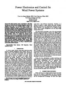
Buck-Boost AC-DC converter at near unity power factor: simulation and experimental results Vsmax = 60V, Rf=0.1 Ω, Lf=5mH, Cf=15μF, Lo=10mH, Co=5000μF 8 6
Vs is
Vs is
1 Voltage*10 [V] ; Current [A]
4 2 2 0 -2
Power factor (Vs-20V/Div) ( is-2A/Div)
-4 -6 -8 0.02
0.025
0.03
0.035
0.04
0.045 0.05 Time [s]
0.055
0.06
0.065
0.07
Experimental
Simulations 80 70
Voltage [V]
50
VCor
VCor VCo 1
60
2
40 30 20 10 0
0
0.2
0.4
0.6
0.8
1 1.2 Time [s]
1.4
1.6
1.8
VCo
Output voltage response (VCor-20V/Div) (VCo-20V/Div),
2
Source: PhD Vitor Pires Fernando A. Silva (
[email protected])
Source: PhD Vitor Pires Advanced Control Methods for Power Electronics and Power Quality
6
Example 1b): Three - Phase Single - Stage Buck-Boost Rectifier Topologies Do iDo
Three-Phase Single-Stage ac/dc Buck-Boost Converter with Six Switches
S1 VS1 VS2 VS3
Ls , Rs
is1
iC
f1
iCo
iC
CF
LO
VO
CO
f2 i rec3
iC
CF
f3
S5
S4
+
S6
CF
iDo o
S1 Vs1
Three-Phase Single-Stage ac/dc Buck-Boost Converter with Four Switches and split inductor/capacitor
Vs2 Vs3
is1
is2 is3
_
iLo
irec2
Ls , Rs
is3
S3
irec1
Ls , Rs
is2
S2
io
Lf , Rf
S2
Lo1 ψo1
irec1 iC
Lf , Rf
f1
iC
VLo1 2
iC o 1 1 Co1
VC o 1
-
f2
load
Cf
C f1
Cf
V
C f2
iLo 2
irec3 iC
V
Do
irec2
Lf , Rf
Cf
iLo 2
io
f3
V
S3
S4
Lo2 ψ o2
C f3
Vo
+ VC o 2
V Lo 2 2
Co2
Do
Source: PhD Vitor Pires Fernando A. Silva (
[email protected])
Advanced Control Methods for Power Electronics and Power Quality
7
L O A D
Experimental Results using sliding mode, PI and Fuzzy Logic DC voltage control 83
82
81
80
79
78
77 0.2
1 - Input source voltage (20V/Div), 2 - Input line current ( 2A/Div)
Input line currents (is1, is2, is3)
0.25
0.3
0.35
0.4
0.45
0.5
0.55
0.6
0.65
Rectifier output voltage response to load change
0.7
PI
83
82
81
80
79
PI
78
SMA
1 - Output voltage reference (10V/Div) 2 - Rectifier output voltage (10V/Div) Fernando A. Silva (
[email protected])
77 0.2
0.25
0.3
0.35
0.4
0.45
0.5
0.55
0.6
0.65
0.7
FLC Rectifier output voltage response to load change
Advanced Control Methods for Power Electronics and Power Quality
Source: PhD Vitor Pires
8
Example 1c): Single-stage isolated rectifier with high power factor (H. M.) iCI
vCI
Select switching variables:
d p1
⎧ ⎪1 ⎪ =⎨ ⎪0 ⎪⎩
(T1 ∨ D1 )on (T3 ∧ D3 )off (T3 ∨ D3 )on (T1 ∧ D1 )off
d p2
⎧ ⎪1 ⎪ =⎨ ⎪0 ⎪⎩
iS1
(T2 ∨ D2 )on (T4 ∧ D4 )off (T4 ∨ D4 )on (T2 ∧ D2 )off
T1
iS2
D1
T2
D2
n:1
+ CI
Write switched state model, function of switching variables:
A LA DA
T3
vA
vB
B T4
D4
D3
DB iLA
iLB
vs
iLo Lo
Co Ro
d d d d ir = (iLA + iLB ) = iLA + iLB dt dt dt dt v Lo vs − vo d p1 − d p 2 vCI − nvo d iLo = = = dt Lo Lo nLo
LB
vo vr ir
i −i d vo = Lo Ro dt Co Source: SPP Hugo Marques Fernando A. Silva (
[email protected])
Advanced Control Methods for Power Electronics and Power Quality
9
Example 1c): Non-linear decision current mode control iCI
Define control variables and errors:
iS1 T1
eir = ir − ir _ ref eiLo = iLo − iLo _ ref
iS2
D1
T2
D2
n:1
+ CI
A LA
Analyze circuit dynamics:
DA
State
dp1
dp2
vAB
di LA dt
di LB dt
dir dt
di Lo dt
1 2 3 4
0 0 1 1
0 1 0 1
0 -VC VC 0
≥0 ≥0 ≤0 ≤0
≥0 ≤0 ≥0 ≤0
≥0 ≈0 ≈0 ≤0
0 >0 0
vB
B T4
D4
D3
LB DB
iLB
vs
iLo Lo
Co Ro vo
no
eir > 0
T3
vA
iLA
Devise a non-linear control decision process: yes
vCI
vr ir
iLA > iLB
yes
no
yes
no
dp1=1 dp2=1
dp1=0 dp2=0
dp1=1 dp2=0
dp1=0 dp2=1
Fernando A. Silva (
[email protected])
Advanced Control Methods for Power Electronics and Power Quality
10
Example 1c): Power Factor and Output Voltage Control 1) POWER FACTOR CONTROL PCI = PI − Po vCI C I
2P d VI d VI 2 vCI = r r − Po ⇔ vCI = r r − o dt 2 dt CI CI
Input current amplitude linear control system: a) mathematical model; b) practical implementation
2) OUTPUT VOLTAGE: LINEAR CONTROL SYSTEM Since ir≈ir_ref and iLo≈iLo_ref, the equivalent circuit is i o
iLo_ref
iCO
Co R0
vo
v0 (s ) R0 = iLo _ ref (s ) sCo R0 + 1
PI controllers selected to impose a 2nd order dynamics with 0.7 damping Fernando A. Silva (
[email protected])
Advanced Control Methods for Power Electronics and Power Quality
11
Example 1c): Results iR
iLA, iLB
v o
VCL iL0
Figure 6 - Controlled system Vo_ref step response. (Vo_ref : 100V to 150V at t = 1sec)
Figure 7 - Expanded scale of Figure 6 results
Figure 8 - Controlled system response to load step disturbance. (Ro : 6.15Ω to 12.3Ω at t = 1 sec). Source: SPP Hugo Marques
Fernando A. Silva (
[email protected])
Advanced Control Methods for Power Electronics and Power Quality
12
Example 2: Three-phase neutral point clamped (NPC) converters io
i I1
iC1
S11 C1
UC1
S12 um1 D11
S21
I2
iC2 UC2
S13 C2
S31
S22
S32
D21
D31
um2
Udc
I3
S23
L
S33 D32
S14
S24
S34
~ us2
L
R
~
Us3
U23 i3
us1
Us2
U12 i2
R
um3
D22
I'2
i1
U31
D12
I'1
Us1
L
R
us3 ~
I'3
•3 level line to neutral voltages •5 level line to line voltages •UC1, UC2 need voltage balancing Fernando A. Silva (
[email protected])
Advanced Control Methods for Power Electronics and Power Quality
13
Switched state-space model of three-phase NPC converters: Steps 1, 2 Step 1) State variables of the power converter: i1, i2, UC1, UC2 ⎧ 1 if (Sk1 ∧ Sk2 ) are ON ⎪ γ k (t ) = ⎨ 0 if (Sk2 ∧ Sk3 ) are ON ⎪- 1 if (S ∧ S ) are ON k3 k4 ⎩
Step 2) Select switching variables to each converter leg: io
Write voltages and currents as functions of γk
i I S11 1
iC1 C1
UC1
S12 um1 D11
I S21 2 S22 D21 um2
Udc iC2 UC2
S13 C2
S23
I3 S31
U31
i2
R
S33
L
S14
S24
S34 I'3
~
R
us2 ~
Us3
U23 i3
us1
Us2
um3
D12
Fernando A. Silva (
[email protected])
L
U12
D31
D32
I'2
i1
S32
D22
I'1
Us1
L
R
us3 ~
Leg voltages: ⎧ U C1 if γ k = 1 ⎪ umk (t ) = ⎨ 0 if γ k = 0 ⎪- U ⎩ C 2 if γ k = −1 Leg currents: ⎧− i if γ k = 1 I k (t ) = ⎨ k if γ k ≠ 1 ⎩0 ⎧ i if γ k = −1 I 'k (t ) = ⎨ k ⎩0 if γ k ≠ −1
Advanced Control Methods for Power Electronics and Power Quality
14
Switched state-space model of three-phase NPC converters: end of step 2 Write voltages and currents depending on γk Leg Voltages:
u mk =
γk 2
(1 + γ k )U C1 + γ k (1 − γ k )U C 2 = Γ1kU C1 + Γ2kU C 2 2
Ik = −
Leg Currents
I 'k = − io
i I S11 1
iC1 C1
UC1
S12 um1 D11
S21
I2
iC2 UC2
S13
S32
D21
D31
C2
S23
S33 D32
S14
S24
S34
Fernando A. Silva (
[email protected])
2
(1 − γ k )ik
i1
L
L
R
us1 ~ us2 ~
k (1 + γ k ) Γ = 1 k where: 2
γ Γ2k = k (1 − γ k ) 2
Us3
U23 i3
= −Γ2 k ik
γ
Us2
U12 i2
R
um3
D22
I'2
γk
(1 + γ k )ik = −Γ1k ik
Us1
U31
D12
I'1
2
I3 S31
S22
um2
Udc
γk
L
R
us3 ~
with Γ1k∈{0, 1}, e Γ2k∈{-1, 0}
I'3 Advanced Control Methods for Power Electronics and Power Quality
15
Step 3) Switched state-space model of threephase NPC converters in system coordinates Step 3) Apply Kirchhoff’s laws
DC side dynamics:
Considering voltage US=Ξ [UC1, UC2]T
AC side dynamics:
Switched statespace model in three phase coordinates:
Fernando A. Silva (
[email protected])
⎡ Γ11 − d ⎡U C1 ⎤ ⎢ C1 =⎢ dt ⎢⎣U C 2 ⎥⎦ ⎢− Γ21 ⎢⎣ C 2
Γ12 C1 Γ − 22 C2 −
Γ13 C1 Γ − 23 C2 −
1 ⎤ ⎡ i1 ⎤ ⎢ ⎥ C1 ⎥ ⎢i2 ⎥ ⎥ 1 ⎥ ⎢i3 ⎥ C 2 ⎥⎦ ⎢⎣io ⎥⎦
⎡ Ξ11 Ξ12 ⎤ ⎡ 2Γ11 − Γ12 − Γ13 1 where Ξ = ⎢⎢Ξ 21 Ξ 22 ⎥⎥ = ⎢⎢− Γ11 + 2Γ12 − Γ13 3 ⎢⎣Ξ 31 Ξ 32 ⎥⎦ ⎢⎣− Γ11 − Γ12 + 2Γ13
U Sk = R ik + L
⎡ R ⎢−L ⎢ ⎡ i1 ⎤ ⎢ 0 ⎢ i ⎥ ⎢ 2 ⎥ ⎢ d ⎢ ⎢ i3 ⎥ = ⎢ 0 dt ⎢ ⎥ ⎢ ⎢U C1 ⎥ ⎢ − Γ11 ⎢⎣U C 2 ⎥⎦ ⎢ C1 ⎢ Γ21 ⎢− C 2 ⎣
0 −
R L
0 Γ12 C1 Γ − 22 C2 −
2Γ21 − Γ22 − Γ23 ⎤ − Γ21 + 2Γ22 − Γ23 ⎥⎥ − Γ21 − Γ22 + 2Γ23 ⎥⎦
dik + u sk dt 0 0
R L Γ13 − C1 Γ − 23 C2 −
Ξ11 L Ξ 21 L Ξ 31 L 0 0
Ξ12 ⎤ ⎡ 1 ⎥ ⎢− L L Ξ 22 ⎥ ⎡ i1 ⎤ ⎢ ⎥ ⎢ 0 L ⎥⎢ i ⎥ ⎢ Ξ 32 ⎥ ⎢ 2 ⎥ ⎢ ⎢ i ⎥+ 0 L ⎥⎢ 3 ⎥ ⎢ ⎥ U ⎢ 0 ⎥ ⎢ C1 ⎥ ⎢ 0 ⎥ ⎢⎣U C 2 ⎥⎦ ⎢ ⎥ ⎢ 0 ⎥ ⎢ 0 ⎣ ⎦
Advanced Control Methods for Power Electronics and Power Quality
0 −
1 L
0
0 0 −
1 L
0
0
0
0
⎤ 0 ⎥ ⎥ 0 ⎥ ⎡u ⎤ ⎥ ⎢ s1 ⎥ u 0 ⎥⎢ s2 ⎥ ⎥ ⎢u ⎥ s3 1 ⎥⎢ ⎥ ⎥ i C1 ⎥ ⎣ o ⎦ 1 ⎥ C 2 ⎥⎦
16
Step 4) Non-linear controller design (n-Level Sliding Mode Control) 4.
A) Transform the switched state-space model into a controllability model d [xi,..., xm-1, xm]T = [xi+1, ..., xm, - ƒi(x) - pi(t)+bi(x) ui(t)]T dt
Define an error vector e=[exi,exi+1,...,exm]T state model, where exo= xor - xo d [exi,...,exm-1,exm]T=[exi+1,...,exm,+ƒi(e)+pei(t)- bei(e)ui(t)]T dt
4.
B) Sliding surface Control law
4.
S(e, t) =
∑o = i ko ex
C) Sliding mode stability
D) 2 level switching law ⎧ U be se S (e, t ) > +ε ui (t ) = ⎨ ⎩ − U be se S (e, t ) < −ε
Fernando A. Silva (
[email protected])
o
=0
S(e, s) = exi (s+ωo)m-i
Reaching mode condition 4.
m
S(e, t) S&(e, t) < 0 d e =ƒ (e)+pei(t)-bei(e)ui(t) ⇒ ui(t) ≥ uieqmax ≥U d t xm i
n level switching law ⎧⎪U j +1 (t ) se S (e, t ) > +ε ∧ S& (e, t ) > +ε ∧ j < n U j (t ) = ⎨ ⎪⎩ U j −1 (t ) se S (e, t ) < −ε ∧ S& (e, t ) < −ε ∧ j > 1
Advanced Control Methods for Power Electronics and Power Quality
17
Step 4 A) Transform the switched state-space model of three-phase NPC converters to α,β coordinates Concordia Transformation
[C] =
⎡ 1 0 1 2 ⎢ ⋅ ⎢− 1 2 3 2 1 3 ⎢ −1 2 − 3 2 1 ⎣
Switched statespace model in α,β coordinates:
• nonlinear • time variant
[Xα, Xβ, X0]T=[C]-1[X1, X2, X3]T
2⎤ ⎥ 2⎥ 2⎥ ⎦
⎡ R ⎢−L ⎡ iα ⎤ ⎢ ⎢i ⎥ ⎢ 0 d ⎢ β ⎥ ⎢ = dt ⎢U C1 ⎥ ⎢⎢ − Γ1α ⎢ ⎥ C1 ⎣U C 2 ⎦ ⎢ ⎢ Γ2α ⎢− C 2 ⎣
Fernando A. Silva (
[email protected])
0 R L Γ1β
− − −
C1 Γ2 β C2
Γ1α L Γ1β L 0 0
Γ2α L Γ2 β
⎤ ⎡ 1 ⎥ ⎢− L ⎥⎡ i ⎤ ⎢ ⎥⎢ α ⎥ ⎢ 0 L ⎥ ⎢ iβ ⎥ ⎢ ⎥ ⎢U ⎥ + ⎢ 0 ⎥ C1 ⎢ 0 ⎢ ⎥ ⎥ ⎣U C 2 ⎦ ⎢ ⎥ ⎢ 0 0 ⎥ ⎢⎣ ⎦
Advanced Control Methods for Power Electronics and Power Quality
0 −
1 L
0 0
⎤ 0 ⎥ ⎥ 0 ⎥ ⎡u sα ⎤ ⎥⎢ ⎥ 1 ⎥ ⎢u sβ ⎥ C1 ⎥ ⎢⎣ io ⎥⎦ 1 ⎥⎥ C 2 ⎥⎦
18
Step 4 A) Transform the NPC converter α,β switched state-space model to d,q coordinates Blondel-Park transformation (d,q)
State-space model in d,q coordinates:
• nonlinear • time invariant
[Xd, Xq]T=[D]-1[Xα, Xβ]T
⎡ R ⎢−L ⎡ id ⎤ ⎢ ⎢ i ⎥ ⎢ −ω d ⎢ q ⎥ ⎢ =⎢ Γ ⎢ ⎥ U dt C1 − 1d ⎢ ⎢ ⎥ C1 ⎣U C 2 ⎦ ⎢ ⎢ Γ2 d ⎢− C 2 ⎣
Fernando A. Silva (
[email protected])
ω R L Γ1q
− − −
C1 Γ2 q C2
Γ1d L Γ1q L 0 0
cos ωt ⎣sen ωt
− sen ωt ⎤ cos ωt ⎥⎦
[D] = ⎡⎢
Γ2 d ⎤ ⎡ 1 ⎢− L L ⎥ Γ2 q ⎥ ⎡ id ⎤ ⎢ ⎥⎢ ⎥ ⎢ 0 L ⎥ ⎢ iq ⎥ ⎢ ⎥ ⎢U ⎥ + ⎢ 0 ⎥ C1 ⎢ 0 ⎢ ⎥ ⎥ ⎣U C 2 ⎦ ⎢ ⎥ ⎢ 0 0 ⎥ ⎢⎣ ⎦
Advanced Control Methods for Power Electronics and Power Quality
0 −
1 L
0 0
⎤ 0 ⎥ ⎥ 0 ⎥ ⎡u sd ⎤ ⎥ ⎢u ⎥ 1 ⎥ ⎢ sq ⎥ C1 ⎥ ⎢⎣ io ⎥⎦ 1 ⎥⎥ C 2 ⎥⎦
19
Step 4 A) Simplify the NPC converter α,β state model into a controllability model Supposing balanced UC1 and UC2 ( UC1≈UC2≈Udc/2 ) ⎡R ⎢L d ⎡iα ⎤ = − ⎢ ⎥ ⎢ dt ⎣iβ ⎦ ⎢0 ⎣
U Sα , β
⎡1 ⎤ 0 ⎥ ⎡u ⎤ ⎢ sα + ⎢L ⎢ ⎥ ⎥ 1 ⎣u sβ ⎦ ⎢0 ⎥ L⎦ ⎣
⎡1 ⎤ 0 ⎥ ⎡i ⎤ ⎢ α − ⎢L ⎥ ⎢ ⎥ R ⎣iβ ⎦ ⎢0 ⎥ L⎦ ⎣
1 ⎡ 1 − ⎡U sα ⎤ 2⎢ 2 = =⎢ ⎢ ⎥ 3 3⎢ ⎣U sβ ⎦ 0 ⎢⎣ 2
⎤ 0 ⎥ ⎡U ⎤ sα ⎢ ⎥ 1 ⎣U sβ ⎥⎦ ⎥ L⎦
1 ⎤ ⎡Λ ⎤ 1 ⎥ ⎢ 2 Λ ⎥ U dc = ⎡ Λ α ⎤ U dc ⎥ ⎢Λ ⎥ 3⎥ ⎢ 2⎥ 2 ⎣ β⎦ 2 − ⎢⎣ Λ 3 ⎥⎦ 2 ⎥⎦ −
2 1 1 2 1 1 2 1 1 Λ1 = γ 1 − γ 2 − γ 3 ; Λ 2 = γ 2 − γ 3 − γ 1 ; Λ 3 = γ 3 − γ 1 − γ 2 ; 3 3 3 3 3 3 3 3 3 T −1 T Λα , Λ β , Λ 0 = [C] [Λ1 , Λ 2 , Λ 3 ]
[
]
Fernando A. Silva (
[email protected])
Advanced Control Methods for Power Electronics and Power Quality
20
Step 4 B) C) and D) Control laws, stability and switching laws for three-phase AC current control 4.
S (ei α , t ) = k i α (iαref − iα ) = k i α ei α = 0 S (ei β , t ) = k i β (i βref − i β ) = k i β ei β = 0
B) Control laws
⎡ ⎛& R 1 1 ⎞⎤ k i i u U + + − ⎡ S& (eiα , t )⎤ ⎢ iα ⎜⎝ αref L α L sα L sα ⎟⎠ ⎥ ⎥ ⎥=⎢ ⎢& R 1 1 ⎢⎣ S (eiβ , t )⎥⎦ ⎢k ⎛⎜ i& + i + u − U ⎞⎟⎥ ⎢⎣ iβ ⎝ βrref L β L sβ L sβ ⎠⎥⎦
4.
C) Sliding mode stability
4.
D) n level switching law (n=5)
⎧⎪S (eiα , β , t ) > ε ⇒ S& (eiα , β , t ) < 0 ⇒ U sα , β > (Li&α , βref + Riα , β + u sα , β ) ⎨ & ⎪⎩S (eiα , β , t ) < −ε ⇒ S (eiα , β , t ) > 0 ⇒ U sα , β < (Li&α , βref + Riα , β + u sα , β )
Fernando A. Silva (
[email protected])
Advanced Control Methods for Power Electronics and Power Quality
21
Step 4 D) Switching laws for three-phase AC current control and space vectors (SV) ⎧ 1 if (Sk1 ∧ Sk2 ) are ON ⎪ γ k (t ) = ⎨ 0 if (Sk2 ∧ Sk3 ) are ON ⎪- 1 if (S ∧ S ) are ON k3 k4 ⎩
Ternary switching variables
3 converter legs ⇒ γ1, γ2, γ3 ⇒ 33 = 27 output voltage vectors io
i
I S11 1
iC1 C1
UC1
S12 um1 D11
S21
I2
S22
S32
D21
D31
um2
Udc iC2 UC2
S13 C2
I3 S31
S23
S33 D32
S14
S24
S34
Fernando A. Silva (
[email protected])
L
L
~
R
us2 ~
Us3
U23 i3
us1
Us2
U12 i2
R
um3
D22
I'2
i1
U31
D12
I'1
Us1
L
R
us3 ~
I'3
Advanced Control Methods for Power Electronics and Power Quality
22
Step 4 D) Space vector table (three wire) r v
γ 1 γ 2 γ 3 S11 S12 S13 S14 S21 S22 S23 S24 S31 S32 S33 S34 um1
1 2 3 4 5 6 7 8 9 10 11 12 13 14 15 16 17 18 19 20 21 22 23 24 25 26 27
1 1 1 1 1 1 1 1 1 0 0 0 0 0 0 0 0 0 -1 -1 -1 -1 -1 -1 -1 -1 -1
1 1 1 0 0 0 -1 -1 -1 -1 -1 -1 0 0 0 1 1 1 1 1 1 0 0 0 -1 -1 -1
1 0 -1 -1 0 1 1 0 -1 -1 0 1 1 0 -1 -1 0 1 1 0 -1 -1 0 1 1 0 -1
1 1 1 1 1 1 1 1 1 0 0 0 0 0 0 0 0 0 0 0 0 0 0 0 0 0 0
1 1 1 1 1 1 1 1 1 1 1 1 1 1 1 1 1 1 0 0 0 0 0 0 0 0 0
0 0 0 0 0 0 0 0 0 1 1 1 1 1 1 1 1 1 1 1 1 1 1 1 1 1 1
0 0 0 0 0 0 0 0 0 0 0 0 0 0 0 0 0 0 1 1 1 1 1 1 1 1 1
Fernando A. Silva (
[email protected])
1 1 1 0 0 0 0 0 0 0 0 0 0 0 0 1 1 1 1 1 1 0 0 0 0 0 0
1 1 1 1 1 1 0 0 0 0 0 0 1 1 1 1 1 1 1 1 1 1 1 1 0 0 0
0 0 0 1 1 1 1 1 1 1 1 1 1 1 1 0 0 0 0 0 0 1 1 1 1 1 1
0 0 0 0 0 0 1 1 1 1 1 1 0 0 0 0 0 0 0 0 0 0 0 0 1 1 1
1 0 0 0 0 1 1 0 0 0 0 1 1 0 0 0 0 1 1 0 0 0 0 1 1 0 0
1 1 0 0 1 1 1 1 0 0 1 1 1 1 0 0 1 1 1 1 0 0 1 1 1 1 0
0 1 1 1 1 0 0 1 1 1 1 0 0 1 1 1 1 0 0 1 1 1 1 0 0 1 1
0 0 1 1 0 0 0 0 1 1 0 0 0 0 1 1 0 0 0 0 1 1 0 0 0 0 1
Udc/2 Udc/2 Udc/2 Udc/2 Udc/2 Udc/2 Udc/2 Udc/2 Udc/2 0 0 0 0 0 0 0 0 0 -Udc/2 -Udc/2 -Udc/2 -Udc/2 -Udc/2 -Udc/2 -Udc/2 -Udc/2 -Udc/2
um2
um3
u12
u23
u31
uα/Udc
uβ/Udc
Udc/2 Udc/2 Udc/2 0 0 0 -Udc/2 -Udc/2 -Udc/2 -Udc/2 -Udc/2 -Udc/2 0 0 0 Udc/2 Udc/2 Udc/2 Udc/2 Udc/2 Udc/2 0 0 0 -Udc/2 -Udc/2 -Udc/2
Udc/2 0 -Udc/2 -Udc/2 0 Udc/2 Udc/2 0 -Udc/2 -Udc/2 0 Udc/2 Udc/2 0 -Udc/2 -Udc/2 0 Udc/2 Udc/2 0 -Udc/2 -Udc/2 0 Udc/2 Udc/2 0 -Udc/2
0 0 0
0
0 -Udc/2 -Udc -Udc -Udc/2 0 0 -Udc/2 -Udc -Udc/2 0 Udc/2 Udc/2 0 -Udc/2 -Udc/2 0 Udc/2 Udc Udc/2 0 0 Udc/2 Udc Udc Udc/2 0
0,000 0,204 0,408 0,612 0,408 0,204 0,408 0,612 0,816 0,408 0,204 0,000 -0,204 0,000 0,204 0,000 -0,204 -0,408 -0,816 -0,612 -0,408 -0,204 -0,408 -0,612 -0,408 -0,204 0,000
0,000 0,354 0,707 0,354 0,000 -0,354 -0,707 -0,354 0,000 0,000 -0,354 -0,707 -0,354 0,000 0,354 0,707 0,354 0,000 0,000 0,354 0,707 0,354 0,000 -0,354 -0,707 -0,354 0,000
Udc/2 Udc/2 Udc/2 Udc Udc Udc Udc/2 Udc/2 Udc/2 0 0 0 -Udc/2 -Udc/2 -Udc/2 -Udc -Udc -Udc -Udc/2 -Udc/2 -Udc/2 0 0 0
Udc/2 Udc Udc/2 0 -Udc/2 -Udc -Udc/2 0 0 -Udc/2 -Udc -Udc/2 0 Udc/2 Udc Udc/2 0 0 Udc/2 Udc Udc/2 0 -Udc/2 -Udc -Udc/2 0
Advanced Control Methods for Power Electronics and Power Quality
23
Step 4 D) α, β space vectors (three-wire)
21
1,0 0,8
beta 16
3
0,6 20
4 17 ; 22 0,4 2;15 B 0,2 19 18 ;23 9 alfa 5;10 1;14;270 -1,0 -0,8 -0,6 -0,4 0,2 0,4 0,6 0,8 1,0 13 ;26 6;11 24 -0,4 8 -0,6 7 25 -0,8 12 -1,0
8 redundant vectors (from the load viewpoint) vectors in red discharge C1 (inverter operation) vectors in blue charge C1 (inverter operation) Fernando A. Silva (
[email protected])
Advanced Control Methods for Power Electronics and Power Quality
24
Step 4 D) Switching law and α,β space vector selection Switching law: ⎧⎪(λαβ ) j +1 = (λαβ ) j +1 if S(eαβ , t) > ε ∧ S& (eαβ , t) > ε ∧ (λαβ ) j < 2 ⎨ ⎪⎩(λαβ ) j +1 = (λαβ ) j −1 if S(eαβ , t) < −ε ∧ S& (eαβ , t ) < −ε ∧ (λαβ ) j > −2
λβ \ λα
-2
-1
0
1
2
-2
25
25
12
7
7
-1
24
13;26
6;11
8
0
19
18;23
13;6 26;11 1;14;27
5;10
9
1
20
17;22
2;15
4
2
21
21
17;2 22;15 16
3
3
Fernando A. Silva (
[email protected])
21
1,0 0,8
beta 16
3
0,6 20
4 17 ; 22 0,4 2;15 B 0,2 19 18 ;23 9 alfa 0 5;10 1;14;27 -1,0 -0,8 -0,6 -0,4 0,2 0,4 0,6 0,8 1,0 13 ;26 6;11 24 -0,4 8 -0,6 7 25 -0,8 12 -1,0
Advanced Control Methods for Power Electronics and Power Quality
25
Step 4 D) Switching law and α,β space vector selection with equalization of UC1 and UC2 Redundant vectors are used to balance UC1 and UC2.
(
Sliding mode control law
Switching law
S(eUc,t)=kU (UC1-UC2)=0
)
⎧IF S eU c , t > +ε U ⇒ Charge C 2 ⎪ ⎪ Zero vectors ⎨IF − ε U < S eU c , t < +ε U ⇒ if possible ⎪ ⎪⎩IF S eU c , t < −ε U ⇒ Charge C1
(
)
(
)
Example: IF UC1>UC2 ⇒ discharge C1 Upon the value of vector [ϒ1, ϒ2] =[(γ1 /2)(γ1+1)-(γ3/2)(γ3+1), (γ2 /2)(γ2+1)-(γ3/2)(γ3+1)]: •Pick-up vector from table 1, if inverter operation:
(UC1>UC2) (ϒ1 i1 +ϒ2 i2)>0 ->{2, 5, 6, 13, 17, 18}
•Pick-up vector from table 2, if rectifier operation: (UC1-UC2) (ϒ1 i1 +ϒ2 i2){10, 11, 15, 22, 23, 26}
Example: IF UC1>UC2 and λα= -1, λ β= -1 and inverter mode ⇒ vector 13 Table 5. Vectors as function of λα,β if UC1-UC2>0 in inverter mode, or if UC1-UC2