is repeated with a period of T. Event streams can describe all ... Figure 4. Approximated event stream element. Let θ be an event element belonging to the event ...
Advanced Hierarchical Event-Stream Model Karsten Albers, Frank Bodmann and Frank Slomka Embedded Systems / Real-Time Systems, Ulm University {name.surname}@uni-ulm.de
Abstract—Analyzing future distributed real-time systems, automotive and avionic systems, is requiring compositional hard real-time analysis techniques. Well known established techniques as SymTA/S and the real-time calculus are candidates solving the mentioned problem. However both techniques use quite simple event models. SymTA/S is based on discrete events the real-time calculus on continuous functions. Such simple models has been choosen because of the computational complexity of the considered mathematical operations required for real-time analysis. Advances in approximation techniques are allowing the consideration of more expressive descriptions of events. In this paper such a new expressive event model and its analysis algorithm are described. It integrates the models of both techniques. It is also possible in this module to integrate an approximative real-time analysis into the event model. This allows to propagate the approximation through the analysis of a distributed system leading to a much more efficient analysis.
1. M OTIVATION The module-based design processes make it possible to handle the complexity in software and hardware design. Systems are build using a set of closed modules. These modules can be designed and developed separately. Modules have only designated interfaces and connections to other modules of their set. The purpose of modularisation is to split the challenging job of designing the whole system into multiple smaller jobs, allowing the reuse of modules in different designs or to include IP components of third-party vendors. Every module-based design concept requires a well defined interface-concept for connecting the modules. Developing realtime systems requires for this interface-concept to cover also the real-time aspects of the modules. A concept for the realtime analysis is required to handle the modules separatly and allows a propagation of the real-time analysis results through the system. It is necessary to propagate the results of the realtime analysis of the different modules in an abstract way. The global analysis is build by connecting the local analyses of the single modules. Therefore it is essiential to have an expressive and efficient interface describing the influence in timing of one module to the next module. One aspect of this interface is the timing description of events which are produced by one module to trigger the next following module. Another aspect is the computation capacity that remains for lower priority modules left over by the higher priority ones. Consider for example a network packet processor as shown in figure 1. The single packages are processed by chains of tasks τ which can be located on different processing elements P. The processing elements P can be processors, dedicated hardware or the communication network. The events Θ triggering the different tasks are equal to the packages
sp
sp
3
P 2
P 1 τ Θ
1
1
τ 4
4
Θ
S
2
2
S τ
Θ
τ Θ
2
Θ Θ
3
4
Θ
Θ
6
S
3
Figure 1.
Θ
τ
5
9
τ
10
6
7 S
3 S
8
6 S
7
τ 5
5
3
P 3
1 S
τ Θ
sp
2
Θ 7
8
11
Θ S
12
8
Network processor example
flowing through the network. Each processing unit P uses a fixed-priority scheduling and the task τ on each unit are sorted by their priority level. Each task τ has, as available capacity, the capacity S! left over by the tasks τ with a higher priority located on the same processing unit. The purpose of this paper is to provide an efficient and flexible approach for the real-time analysis of such a modularized system. Therefore is a powerful and sufficient event model for describing the different time interfaces for the different aspects is necessary. 2. R ELATED WORK The most advanced approach for the real-time analysis of such a modulare network is the real-time calculus by Thiele et al. [4], [13]. It is based on the network calculus approach defined by Cruz [5] and Parekh and Gallager [9]. The event pattern is modeled by an sub-additive upper and super-additive lower arrival curve α uf (Δt) and α lf (Δt) delivering for every Δt the maximum number of events or the minimum, respectivly. The service curves βru (Δt) and βrl (Δt) model the upper and lower bound of the computational requirements which can be handled by the resource during Δt. The real-time calculus provides equations to calculate the outgoing arrival and service curves out of the incoming curves of a task. To evaluate the modification equations independently from each other, a good finit description for the curves is needed. The complexity of the equations depends directly on the complexity of this description. In [8] and [4] an approximation with a fixed degree of exactness for the arrival and service curves was proposed in which each curve is described by three straight line segments. One segment describes the initial offset or arrival time, one an initial burst and one the long time rate.
Δt T ,a, l k Θ θ = (T,a) ˆ Θ θˆ = (T,a,l,G, Θˆ θˆ ) s ˆ Ψ(Δt, Θ) ˆ ϒ(Δt, Θ), ˆ B I (Δt, Θ),
interval period, offset, limitation number of test intervals event stream event element hierachical event stream hierachical event stream element separation point event bound function, demand bound function interval bound function, busy period Table I L IST OF SYMBOLS
Events
Time
Figure 2.
Example Event Stream
As outlined in [3] this approach is too simplified to be suitable for complex systems. No suitable description for the function is known so far. In this paper we will propose a model for the curves having a selectable approximation error. A tradeoff between this degree of accuracy and the necessary effort for the analysis becomes possible. SymTA/S [11],[12] is another approach for the modularized real-time analysis. The idea was to provide a set of interfaces which can connect different event models. Therefore the different modules can use different event models for analysis. Unfortunatly, the event models for which interfaces are provided are quite simple. In [11] an event model covering all these models was described. The problem of these models is that multiple bursts or bursts with different minimum separation times cannot be handled. However in [10] a real-time analysis problem was formulated, which can’t be solved by SymTA/S and the realtime calculus by each technique exclusivly. To solve it, it is necessary to integrate the models of both techniques into one powerful new model. The event stream model proposed by Gresser [7] with its extension the hierachical event stream model proposed by Albers et al. [1] can model systems with all kinds of bursts efficiently. The problem is that it can only model discrete events and not the continious service function as needed for the real-time calculus. . 2.1. Event stream model For the event stream model a system is described by a set of communicating tasks τ . Each task is assigned to one resource ˆ c, d) is given by the worst-case execution time cτ , ρ . τ = (Θ, ˆ τ triggering the tasks the deadline dτ and an event pattern Θ activations. The key question is to find a good model for the event ˆ For real-time analysis this model has to describe the pattern Θ. worst-case densities of all possible event patterns. They lead to the worst-case demand on computation time. Comparing these worst-case demands with the available computation time
Θ5
T
Θ6
T−j
Θ7
t
T
Figure 3.
Example event streams ([6])
allows to predict the schedulability of a system. The event stream model gives an efficient general notation for the event bound function. Definition 1: ([7], [2], [1]) The event bound function ϒ(Δt, Θ) gives an upper bound on the number of events occuring within any interval Δt. Lemma 1: ([7]) The event bound function is a subadditive function, that means for each interval Δt, ΔJ: ϒ(Δt + Δt !, Θ) ≤ ϒ(Δt, Θ) + ϒ(Δt ! , Θ) Proof: The events in Δt + Δt ! have to occure either in Δt or in Δt ! . Definition 2: An event stream Θ is a set of event elements θ = (T, a) given by a period T and an offset a. Θ1 = {(6, 0), (6, 1), (6, 3)} (figure 2) describes three events requiring at least an interval Δt = 3 to occure, two of them ˆ 1 is repeated have a minimum distance of one time unit. Θ with a period of 6. In cases where the worst-case density of events is unknown for a concrete system an upper bound can be used for the event stream. The model can describe any event sequence. Only those event sequences for which the condition of sub-additivity holds are valid event streams. Lemma 2: ([7]) The event bound function for an event sequence Θ and an interval I is given by: ! " Δt − aθ ϒ(Δt, Θ) = ∑ +1 Tθ θ ∈Θ Δt≥aθ
Proof: See [2] It is a monotonic non-decreasing function. A larger intervallength cannot lead to a smaller number of events. In figure 3 some examples for event streams can be found. The first one Θ5 = {(T, 0)} has a strictly periodic stimulus with a period T . The second example Θ6 = {(∞, 0), (T, T − j)} shows a periodic stimulus in which the single events can jitter within a jitter interval of size j. In the third example Θ7 = {(T, 0), (T, 0) , (T, 0), (T,t) } three events occur at the same time and the fourth occurs after a time t. This pattern is repeated with a period of T . Event streams can describe all these examples in an easy and intuitive way. The offset value of the first event element is always zero as this value models the shortest interval in which one single event can occur. For the real-time analysis for this model let us first repeate the demand bound function definition for the event streams: Ψ(Δt, $Γ) = ∑∀τ ∈Γ ϒ(Δt − dτ , Θτ )cτ # Δt−aθ −dτ = ∑∀τ ∈Γ ∑ ∀θ ∈Θτ + 1 cτ T Δt≥aθ +dτ
θ
Costs
} cτ
ψ (Δ t ,τ,κ) ψ(Δ t ,τ)
}
κ cτ
I Figure 4.
analysis algorithms, it also allows to propagate the approximation together with the event models through the distributed system leading to an efficient, flexible and powerful analysis methodology for distributed real-time systems. The new model can, of course, also model the service functions of the realtime calculus in the same flexible way and allows therefore the integration of the discrete event model of SymTA/S with the continuous service functions.
Approximated event stream element
4. M ODEL Let θ be an event element belonging to the event stream Θ which belongs to the task τ . The demand bound function allows a schedulability analysis for single processor systems by testing ∀Δt : Ψ(Δt, Γ) ≤ C (Δt). Often an idealized capacity function C with C (Δt) = Δt is assumed. For an efficient analysis an approximation is necessary 2.2. Approximation of event streams Definition 3: ([2]) Approximated event-bound-function Let k be a chosen number of steps which should be considered exactly. Let Δtθ ,k = dτ + aθ + kT . We call % ϒ(Δtθ ,k , θ ) + Tcτ (Δt − Δt) Δt > Δtθ ,k θ ϒ! (Δt, θ , τ , k) = Δt ≤ Δtθ ,k ϒ(Δt, θ ) the approximated event bound function for task τ . The function is shown in figure 4. The first k events are evaluated exactly, the remaining events are approximated using cτ the specific utilization Uθ = T θ . The interesting point of this θ function is that the error can be bounded to εθ ,k = 1k and therefore does only depend on the chooseable number of steps, and is independent of the concrete values of the parameters of the tasks. The complete approximated demand-bound-function is Ψ! (Δt,Γ,k)=∑∀τ ∈Γ ∑∀θ ∈Θτ Ψ! (Δt,θ ,k) and has the same error. The hierachical event stream model [1] extends the event stream model and allows a more efficient description of bursts. In this model an event element describes the arrival not for just one periodic event but of a complete set of periodic events. This set of events can be also modeled by an event sequence having a limitation in the number of events generated by this event sequence. One limit of this model is that it can only describe discrete events. For the approximation it would be appropriate for the model to be capable to describe also the continuous part of the approximated event bound function. 3. C ONTRIBUTION In this paper we will present an event model covering both, the discrete event model of SymTA/S and the continuous functions of the real-time calculus. It makes the elegant and tighter description of event bursts compared to the SymTA/S approach possible and allows a tighter modeling of the continuous function of the real-time calculus by integrating an approximation with a chooseable degree of exactness into the model. This does not only lead to more flexible and simpler
We will define the hierachical event sequence first. The hierarchical event stream is only a specialised hierachical event sequence fulfilling the condition of sub-additivity and can therefore be described by the same model. ˆ = {θˆ } conDefinition 4: A hierachical event sequence Θ sists of a set of hierarchical event elements θˆ each describing a pattern of events or of demand which is repeated periodically. The hierarchical event elements are described by: ˆ θˆ = (T, a, l, G, Θ) where Tθ is the period, aθ is the offset, lθ is a limitation of the number of events or the amount of demand generated ˆ ˆ are the time by this element during one period, Gθˆ and Θ θ pattern how the events respectively the demand is generated. The gradient Gθˆ describing a constantly growing set of events, gives the number of events occurring within one time unit. A value Gθˆ = 1 means that after one time unit one event has occured, after two time units two events and so on. The gradient allows modeling approximated event streams as well as modeling the capacity of resources. Both cases can be described by a number of events which occurs respectively ˆ ˆ is again a hierarcan be processed within one time unit. Θ θ chical event stream (child event stream) which is recursively embedded in θˆ . ˆ ˆ = 0/ or G ˆ = 0. Condition 1: Either Θ θ θ Due to this condition it is not necessary to distribute the limitation between the gradient and the sub-element. This simplifies the analysis without restricting the modelling capabilities. The arrival of the first event occurs after a time units and at a + T , a + 2T , a + 3T, ..., a + iT (i ∈ N) the other events occurs. Definition 5: A hierarchical event stream fulfills for every ˆ ≤ ϒ(Δt, Θ) ˆ + ϒ(Δt ! , Θ) ˆ Δt, Δt ! the condition ϒ(Δt + Δt !, Θ) In the following we will give a few examples to show the usage and the possibilities of the new model. A simple periodic event sequence with period 5 can be modeled by : ˆ 1 = {(5, 0, 1, 0, e)} Θ Lemma 3: Let Θ be an event stream with Θ = {θ1 , ..., θn }. ˆ = {θˆ1 , ..., θˆn } with θˆi = Θ can be modeled by Θ (Tθi , aθi , 1, ∞, 0) / Proof: Each of the hierarchical event elements generates exactly one event at each of its periods following the pattern of the corresponding event element. ˆ 10 = ˆ 1 approximated after 10 events would be modeled by: Θ Θ 1 1 {(∞, 0, 10, 0, {(5, 2, 1, 0, e)}), (∞, 47, ∞, 5 , 0)} /
... 0
10 Figure 5.
20
30
Events 30
40
Example for overlapping events of different periods
20
Note that 47 = 2 + (10 − 1) · 5 is the point in time in which the last regular event occurs and therefore the start of the approximation. ˆ 2 = {(∞, 0, 1, ∞, 0)}. One single event is modeled by Θ / A gradient of ∞ would lead to an infinite number of events but due to the limitation only one event is generated. An event bound function requiring constantly 0.75 time units processor time within each time unit can be described by / θˆ2 = (∞, 0, ∞, 0.75, 0). With the recursively embedded event sequence any possible pattern of events within a burst can be modeled. The pattern consists of a limited set of events repeated by the period of the parent hierarchical event element. For example a burst of five events in which the events have an intra-arrival rate of 2 time units which is repeated after 50 time units can be modeled by ˆ 3 = {(50, 0, 5, 0, {(2, 0, 1, ∞, 0)})}. Θ / The child event stream can contain grand-child event ˆ 3 is used only for 1000 time units streams. For example if Θ and than a break of 1000 time units is required would be ˆ 4 = {(2000, 0, 100, 0, Θ ˆ 3)}. modeled by Θ The length Δtθˆ of the interval for which the limitation of θˆ is reached can be calculated using a interval bound function ˆ = min(Δt|x = ϒ(Δt, Θ)) ˆ which is the inverse function I (x, Θ) to the event bound function (I (l, 0) / = 0): ˆ ˆ ) + lθˆ Δtθˆ = I (l, Θ θ Gθˆ Note that this calculation requires the condition of the model ˆ ˆ = 0/ and that the calculation of the that either Gθˆ = 0 or Θ θ interval bound function requires the distribution of lθˆ on the ˆ ˆ. elements of Θ θ 4.1. Assumptions and Condition For the analysis it is useful to restrict the model to event sequences having no overlapping periods. Consider for example (figure 5) θˆ5 = {(28, 0, 15, 0, {(3, 0, 1, ∞, 0)})}. / The limitation interval Δtθˆ6 has the length Δtθˆ6 = (15 − 1) · 3 = 42. The first period [0, 42] and the second period [28, 70] of the event sequence element overlap. Condition 2: (Separation Condition) θˆ fulfills the separation condition if the interval in which events are generated by ˆ ˆ is equal or smaller than its period T ˆ : Gθˆ or Θ θ θ ˆ ˆ ) + lθˆ ≤ T ˆ or T ˆ ≤ ϒ(T ˆ , Θ ˆ ˆ ) + Tθˆ I (lθˆ , Θ θ Gθˆ θ θ θ θ Gθˆ The condition 2 does not reduce the space of event patterns that can be modeled by a hierarchical event sequence. Lemma 4: A hierarchical event sequence element θˆ that does not meet the separation condition can be exchanged with ' & I (lθˆ ,θˆ ) ˆ ˆ a set of event sequence elements θ1 , ..., θk with k = Tˆ θ
ˆ ˆ ). and θˆi = (kTθˆ , (i − 1)Tθˆ + aθˆ , lθˆ , Gθˆ , Θ θ Proof: The proof is obvious and therefore skipped.
10
10
20
Figure 6.
30
40
50
60
70
I
ˆ6 Hierarchical event sequence Θ
ˆ! ˆ5 meetcan be transferred into Θ Θ 5 ˆ! ing the separation condition: Θ = 5 {(56, 0, 15, 0, {(3, 0, 1, ∞, 0)}), / (56, 28, 15, 0, {(3, 0, 1, ∞, 0)})} / The separation condition prohibits events of different event sequence elements to overlap. We also do not allow recursion, so no event element can be the child of itself (or a subsequent child element). 4.2. Hierarchical Event Bound Function The event bound function calculates the maximum number ˆ within Δt. of events generated by Θ Lemma 5: Hierarchical Event Bound Function (ϒ(Δt, ) Θ): Let for any Δt, T define mod(Δt, T ) = Δt − Δt T T and ˆ = ∑ θˆ ∈Θˆ ϒ(Δt, θˆ ) and ϒ(Δt, 0) / = 0. Let ϒ(Δt, Θ) Δt≥a ˆ θ
l#θˆ $ Δt−aθˆ + 1 lθˆ T θˆ min(lθˆ , (Δt − aθˆ )Gθˆ ˆ ϒ(Δt, θˆ ) = $ − aθˆ , Θθˆ )) # +ϒ(Δt Δt−aθˆ lθˆ + min(lθˆ , Tθˆ mod(Δt − aθˆ , Tθˆ )Gθˆ +ϒ(mod(Δt − a , T ), Θ ˆ ˆ )) θˆ θˆ θ
Tθˆ = ∞, Gθˆ = ∞ Tθˆ '= ∞, Gθˆ = ∞ Tθˆ = ∞, Gθˆ '= ∞
Tθˆ '= ∞, Gθˆ '= ∞
Proof: Due to the separation condition it is always possible to include the.#maximum $ /allowed number of events Δt−aθˆ for completed periods lθˆ . Only the last incomplete Tθˆ fraction of a period has to be considered separately (min(...)). This remaining interval is given by subtracting 0 all complete pe1 riods, and the offset a from the interval Δt mod(Δt − aθˆ , Tθˆ . For the child event stream, the number of events is calculated by using the same function with now the remaining interval and the new embedded event sequence. In case of the gradient the number of events is simply Gθˆ Δt. The limitation bounds both values due to the separation condition. Independently of the hierarchical level of an event sequence element it is considered only once during the calculation for one interval. This allows bounding the complexity of the calculation. ˆ 6 = {(20, 6, 10, 0, {(3, 0, 2, 1, 0)}. ˆ 7 ) is Example 1: Θ / ϒ(Δt, Θ ˆ 6 ) is given by shown in figure 6. ϒ(33, Θ ! " ˆ ˆ )) ˆ 6 ) = 27 l ˆ + min(l ˆ , mod(27, T ˆ )G ˆ + ϒ(mod(27, T ˆ ), Θ ϒ(33, Θ θ θ θ θ θ Tθˆ θ
" 27 ˆ ˆ )) · 10 + min(10, 0 + ϒ(7, Θ θ 20 ˆ ˆ )) = 10 + min(10, ϒ(7, Θ θ ! " 7 ! ˆ ˆ ϒ(7, Θθˆ )=ϒ(7, θ ) = · 2 + min(2, mod(7, 3) · 1 + 0) = 4 + 1 = 5 3 ˆ 6 ) = 10 + min(10, 5) = 15 ϒ(33, Θ =
!
4.3. Reduction and Normalization In the following we will reduce event streams to a normal form. The hierarchical event stream model allows several different description for the same event pattern. ˆ = {(100, 0, 22, 0, Θ ˆ a)} with For example an event stream Θ ˆ = ˆ / (5, 3, 2, ∞, 0)} / can be rewritten as Θ Θa = {(7, 0, 3, ∞, 0), ˆ ˆ {(100, 0, 12, 0, θa,1), (100, 0, 8, 0, θa,2), (100, 23, 2, ∞, 0)} / with θˆa,1 = (7, 0, 3, ∞, 0) / and θˆa,2 = (5, 3, 2, ∞, 0). / ˆ !a )} with a ˆ a = {(Ta , aa , la , 0, Θ Lemma 6: An event stream Θ ! ! ! ! ! ! ! ˆ ˆ ˆ k )} child element Θa = {(T1 , a1 , l1 , G1 , Θ1 ), ..., (Tk , ak , lk! , G!k , Θ ˆ b with can be transferred into an equivalent event stream Θ ˆ b = {θˆa,1 , θˆa,2 , ..., θˆa,n , θˆa,x } having only child event seΘ quences with one element where ! ! θˆb,i = (T, a, ϒ(Δta , θˆa,i ), 0, θˆa,i ) ! ˆ Δta = lim (I (la , Θa ) − ε )
ε →0 ε >0
ˆ !a ), la − θˆa,x = (∞, I (la , Θ
∑
! ), ∞, 0) / ϒ(Δta , θˆa,i
ˆ !a ∀θˆ ∈Θ
Proof: We have to distribute the limitation la on the elements of the child event sequence. First we have to find the interval Δt ! for which the limitation of the parent element ˆ !a . Δt ! is given by la is reached by the child event sequence Θ ! ˆ I (la , Θa ). We have to calculate the costs required for each of the child event sequence elements for Δt ! . It is given by ϒ(Δt ! , θˆi ). The problem is that several elements can have a gradient of ∞ exactly at the end of Δt ! . In this situation the sum of ϒ(Δt ! , θˆ ) may exceed the allowed limitation la of the parent element. The total costs is bounded by the global limitation la rather than the limitations li! . To take this effect into account we exclude the costs occurring exactly at the end of Δt ! for each hierarchical event element and we handle these costs seperately modeling them with the hierarchical event element θˆa,x . To do so we calculate the limitation not by ϒ(Δt ! , θˆi! ) but by ϒ(Δt ! − ε , θˆi! ) where ε is an infinitly small value excluding only costs occurring at the end of Δt ! exactly. This allows a better comparison between different hierarchical event streams. 4.4. Capacity Function The proposed hierarchical event stream model can also model the capacity of processing elements and allows to describe systems with fluctuating capacity over the time. In the standard case a processor can handle one time unit execution time during one time unit real time. For many resources the capacity is not constant. The reasons for a fluctuating capacity can be for example operation-system tasks or variable processor speeds due to energy constraints.
3000
Costs
Costs
2000 1000
1000 300
a)
2000
I
Costs
t 3000
200
2000
100
1000
100
c)
Figure 7.
200
I
b)
Costs
1000
2000
d)
Example service bound functions
Assuming the capacity as constant also does not support a modularization of the analysis. This is especially needed for hierarchical scheduling approaches. Consider for example a fixed priority scheduling. In a modular approach each priority level gets the capacity left over by the previous priority level as available capacity. The remaining capacity can be calculated step-wise for each priority level taking only the remaining capacities of the next higher priority level into account. Such an approach is only possible with a model that can describe the left-over capacities exactly. Definition 6: The service function β (Δt, ρ ) gives the minimum amount of processing time that is available for processing tasks in any interval of size Δt for a specific resource ρ for each interval Δt. It can also be modeled with the hierarchical event sequence model. The service function is superadditiv and fulfills the inequation β (Δt + Δt ! ) ≥ β (Δt) + β (Δt ! ) for all Δt, Δt ! . The definition matches the service curves of the real-time calculus. We propose to use the hierarchical event stream model as an explicit description for service curves. In the following we will show, with a few examples, how to model fluctuating service functions with the hierarchical event streams. The constant capacity, as shown in 7 a) can be modeled by: βbasic = {(∞, 0, ∞, 1, 0)} / Blocking the service for a certain time t (figure 7 b) is done by: βblock = {(∞,t, ∞, 1, 0)} / A constantly growing service curve in which the service is blocked periodically every 100 time units for 5 time units (for example by a task of the operating system): βT block = {(100, 5, 95, 1, 0)} / (figure 7 c) ) The service for a processor that can handle only 1000 time units with full speed and than 1000 time units with half speed (figure 7 d)): / (2000, 0, 1000, 1, 0)} / βvary = {(2000, 1000, 500, 21 , 0), These are only a few examples for the possibilities of the new model. 4.5. Operations In the following we will introduce some operations on hierarchical event sequences and streams. ˆA+Θ ˆ B than for each ˆC = Θ Lemma 7: (+ operation) If Θ ˆ C ) = ϒ(Δt, Θ ˆ A ) + ϒ(Δt, Θ ˆ B) is interval Δt the equation ϒ(Δt, Θ
I
I
ˆC =Θ ˆ A ∪Θ ˆ B. true. It can be calculated by the union Θ It is also necessary to shift values. Lemma 8: (→ shift-operation) We have 2 ˆ ! ˆ ) = ϒ(Δt − t, Θ) Δt ≥ t ϒ(Δt, Θ 0 else ˆ ! contains and only contains for each element θˆ ∈ Θ ˆ an if Θ ! ! ! ˆ ˆ ˆ ˆ θ ∈ Θ with θ = (Tθˆ , aθˆ + t, lθˆ , Gθˆ , Θθˆ ). ˆ is defined ˆ ! ) = ϒ(Δt + t, Θ) The shift operation (←) ϒ(Δt, Θ ! ˆ ˆ in a similar way with θ = (Tθˆ , aθˆ − t, lθˆ , Gθˆ , Θθˆ ). This operation (←, →) is associative with the (+) operation ˆ A +Θ ˆ B ) → t = (Θ ˆ A → t) + (Θ ˆ B → t) and (Θ ˆA+ so we have (Θ ˆ ˆ ˆ ˆ ΘB ) ← t = (ΘA ← t) + (ΘB ← t). For (Θ → t) → v we can ˆ → (t + v). write also Θ To scale the event stream by a cost value is for example necessary to integration of the worst-case execution times. ˆ ! = cΘ. ˆ Then for each interval Δt: Lemma 9: Let Θ ! ˆ ˆ ˆ ! contains and only ϒ(Δt, Θ ) = cϒ(Δt, Θ) if the child set of Θ ˆ ˆ an element contains for each element θ of the child set of Θ ! ! ! ˆ ˆ ˆ ˆ θ ∈ Θ having θ = (Tθˆ , aθˆ , clθˆ , cGθˆ , cΘθˆ ). Proof: We do the proof for the add-operation: ˆ A ) + ϒ(Δt, Θ ˆ B) ˆ C ) = ϒ(Δt, Θ ϒ(Δt, Θ = ∑ ϒ(Δt, θˆ ) + ∑ ϒ(Δt, θˆ ) ˆA θˆ ∈Θ
=
ˆB ∀θˆ ∈Θ
ˆ A ∪Θ ˆ B) ϒ(Δt, θˆ ) = ϒ(Δt, Θ
∑
ˆ A ∪Θ ˆB ∀θˆ ∈Θ
The other proofs can be done in a similar way. 4.6. Utilization Lemma 10: The utilization UΓ of a task set in which the event generation patterns are described by hierarchical event ˆ τ )|(l ˆ '= ∞ ∨ T ˆ = ∞)): streams is given by ((∀τ ∈ Γ)Λ (∀θˆ ∈ Θ θ θ / . nθˆ UΓ = ∑∀τ ∈Γ ∑∀θˆ ∈Θˆ τ T ˆ + ∑∀τ ∈Γ ∑∀θˆ ∈Θˆ τ UΘˆ ˆ + Gθˆ Tτ '=∞
θ
lθˆ =∞ Tθˆ =∞
θ
Note that event-elements with an infinite period and a finite limitation do not contribute to the utilization. 5. S CHEDULABILITY TESTS For the schedulability tests of uni-processor system using the hierarchical event stream model analysis, we can integrate the approximation and the available capacity into the analysis. 5.1. Schedulability tests for dynamic priority systems A system scheduled with EDF is feasible if for all intervals Δt the demand bound function does not exceed the service function Ψ(Δt) ≤ C (Δt, ρ ). Both, the demand bound and the service function can be described by and calculated out of hierarchical event streams. This leads to the test ∑∀τ ∈Γ ∑∀θˆ ∈Θˆ τ ϒ(Δt − dτ , θˆ )cτ ≤ C (Δt, ρ ). The analysis can be done using the approximation as proposed in [2]. For the exact analysis an upper bound for Δt, a maximum test interval is required to limit the run-time of the test. For the hierarchical event stream model one maximum test interval available is the busy period.
5.2. Response-time calculation for static priority scheduling In the following we will show how a worst-case response time analysis for scheduling with static priorities can be performed with the new model. The request bound function Φ calculates the amount of computation time of a higher priority task that can interfere and therefore delays a lower-priority task within an interval Δt. In contrary to the event bound function the request bound function does only contain the events of the start, not the events of the end point of the interval: Φ(Δt, τ ) = lim (ϒ(Δ, Θτ )cτ ) Δ→Δt 0≤Δ kl ! ˆ◦
θˆ !k = {(∞, 0, klθˆ , 0, θˆ ), (∞, kTθˆ , lθˆ , Gθˆ , 0), / (∞, kTθˆ +
c l
l
lθˆ lˆ , ∞, θ , 0)} / Gθˆ Tθˆ
The calculation of lA , lB , aA , aB and aC are done as follows: 23 ! 4 kl ! l l l ≤ kl lA = l l > kl ! 23 ! 4 kl ! l T + a l ≤ kl aA = T +a l > kl ! aB = kT + a + a! The approximation of θˆ ! can be done by an element θˆ !k ! with a gradient Gθˆ !k = Tl ! . When starting finally the approximation of θˆ a cost-offset x is required to ensure that the approximated function ϒ(Δt, θˆ k ) is always equal or higher than the exact function ϒ(Δt, θˆ ).
T−y
T
I gradient period limitation
x o y
Figure 8.
Case θˆ ! approximated, θˆ not approximated
Figure 8 outlines this situation. This cost-offset is necessary as a new period of the parent element splits the approximation of the child element. The calculation of x can be done as follows: l l−x = y .T y/ x = l 1− T y gives the interval between the start of the child element θˆ ! and the point in time in which the limitation of θˆ is reached. The reaching of the limitation is calculated using the approximative description of the child elements of θˆ with the seperate consideration of every first event of θˆ . For a simple child element θˆ = {(T, a, l, 0, θˆ ! )} with θˆ ! = {(T ! , a! , l ! , ∞, 0)} / this value y is given by (y − a!) · (
l! ) = l − l! T! l − l! l y = l ! + a! = T ! ! − T ! + a! l T! ! 2
!
!
Hence for x: x = l − TT ll! + TT l − aTl Example 3: Let us consider the example hierarchical event ˆ ˆ !)}, Θ ˆ ! ={(10,2,3,∞,0)} sequence: Θ={(80,2,16,0, / Θ ˆ 10 we get the values: For the approximation Θ & ' & !' 10 · 3 kl l= 16 = 32 lA = l 16 & ' & !' 10 · 3 kl aA = T +a = 80 + 2 = 162 l 16 aB = kT + a = 10 · 80 + 2 = 802 16 l y = T ! ! − T ! + a! = 10 − 10 + 2 = 45.3333 l 5 3 6 . y/ 45.333 x = l 1− = 16 1 − = 6.9333 T 80 ˆ 10 = {(∞, 0, 32, 0, {(80, 2, 16, 0, {(10, 2, 3, ∞, 0)})}), Θ / 3 / (∞, 162, 128, 0, {(∞, 2, 3, ∞, 0), / (∞, 2, ∞, , 0), 80 16 3 / (∞, 802, 6.9333, ∞, 0), / (∞, 802, ∞, , 0)} / (80, 2, 13, , 0)}, 10 80
6.3. Approximation of n-level child element Let us consider the following hierarchical event element with two levels of child elements θˆ = {(T, a, l, 0, θˆ ! )}, θˆ ! = {(T ! , a! , l ! , 0, θˆ !! )}, θˆ !! = {(T !! , a!! , l !! , G!! , 0)} / . We consider the approximation θˆ k . θˆ k is given by
θˆ k = {(∞, 0, lA , 0, θˆ ◦ 1 ), (∞, aA , lB , 0, θˆ ◦ 2 ), / (T, a! , l − x! , (∞, aB , lC , 0, {(T, a! , x! , ∞, 0), l / (∞, aC , x, ∞, 0), (∞, aC , ∞, , 0)} T
l! , 0)}), / T!
θˆ ◦ 1 depends on whether l ≤ kl !! or l > kl !! . We have θˆ ◦ 1 =
2 θˆ
{(T, 0, l, 0, θˆ !k )}
l ≤ kl !! l > kl !!
lˆ lˆ θ = {(∞, 0, klθˆ , 0, θˆ ), (∞, kTθˆ , lθˆ , Gθˆ , 0), / (∞, kTθˆ + θ , ∞, θ , 0)} / Gθˆ Tθˆ ˆ !k
θˆ ◦ 2 depends on whether l ≤ kl ! or l > kl ! . We have 2 0/ l ≤ kl ! ◦ ˆ θ 2= !! !! / l > kl ! {(T ! , a!! , l !! , G!! , 0), (T ! , a!! + Gl !! , l ! − l !! , Tl !! , 0)}
The calculation of lA , aA and lB : 23 !! 4 kl l l ≤ kl !! l lA = l l > kl !! 23 ! 4 kl ! l l − lA l ≤ kl lB = 0 l > kl !
ˆ k can be generalized Therefore the proposed description for Θ to handle event sequences with n-level child event sequences. The calculation is visualized in figure 8. Example 4: Let us consider the example hierarchiˆ = {(1000, 10, 100, 0, Θ ˆ !)}, Θ ˆ! = cal event sequence: Θ !! !! ˆ ˆ {(80, 2, 16, 0, Θ )}, Θ = {(10, 2, 3, ∞, 0)}. / ˆ 10 in which k = 10 test intervals are For an approximation Θ considered exactly we get the values: 16 − 3 y! = 0 3 1 + 2 = 45.3333 10 5
6 80 − 45.3333 = 6.9333 80 100 − 6.9333 . / y= + 2 = 467.333
x =16 · !
16 80
x = 100 ·
5
1000 − 67.3335 1000
6
= 53.2667
ˆ 10 ), (∞, 1012, 100, 0, {(∞, 2, 3, ∞, 0), ˆ 10 = {(∞, 0, 100, 0, Θ / Θ 2,1 3 3 / (80, 2, 13, , 0)}), / (∞, 2010, 800, 0, (∞, 2, ∞, , 0), 80 10 6.9333 , 0), / (1000, 2, 93.0667, {(∞, 2, 6.9333, ∞, 0), / (∞, 2, ∞, 1000 100 16 , 0)}), / (∞, 10010, 53.2667, ∞, 0), / (∞, 10010, ∞, , 0)} / 80 1000 10 ˆ Θ2,1 = {(∞, 0, 32, 0, {(80, 2, 16, 0, {(10, 2, 3, ∞, 0)})}), / 3 3 (∞, 162, 3, ∞, 0), / (∞, 162, ∞, , 0), / (80, 162, 13, , 0)} / 80 10
6.4. Approximation of element with several child elements
lC = kl − (lA + lB) 23 !! 4 kl T + a! + a l ≤ kl !! l aA = T + a! + a l > kl !! 23 ! 4 kl l ≤ kl ! l T aB = T l > kl !
A hierarchical event sequence with several child elements can be transferred into a normalized hierarchical event sequence in which each event sequence element has only one child element. Each element matches one of the previous pattern and can therefore be approximated. The overall approximation of the event sequence is than only a merge of the single elements.
aC = kT + a
6.5. Required number of test intervals
x!
The calculation of is the same as the calculation for x in the previous section. We have l! y! = T !! !! − T !! + a!! 5l ! !6 ! ! T −y x =l T! The calculation of x and y is similar but using the approximation of θˆ !! . We have l! (y − a) · ( ! ) = l − x! T lT ! x! T ! y = ! − ! + a! l l6 5 T −y x=l T
Note that when setting x!! = l !! the calculation of x! and y! on the one side and x and y on the other side are the same.
In those cases in which the approximation of the child element starts within the completion of the first period of the parent element we cannot postpone it until the first period of the parent. It would not be possible to bound the number of test intervals for the child hierarchical event element. Example 5: Consider the following example: θˆ10 = {10000, 0, 4000, 0, {θˆ 11}}, θˆ11 = {10, 0, 5, ∞, 0} / Postponing the approximation of the child up to the end of the first period of the parent would cost 3000 additional test intervals. We can still find a simple bound on the required number of test intervals. For those cases in which the approximation does not start within the first period, the number of test intervals for one period of the parent event element has to be less than the approximation bound k. Otherwise the approximation would be allowed somewhere within the first period. Therefore the maximum number of test intervals we have to additionally consider due to the postponing is bounded also by k, so a total bound of 2k.
6.6. Splitting points The splitting points are the points in which the parent element is splitted to destinguish between the non-approximated and the approximated part of one of its child elements. In general, the parent element is splitted at the first of its completed period which is greater than the first possible approximation interval of the child element. Each element can require as many splitting points as its total child-set has members. The total child-set contains its children, the children of its children and so on. The parent chain contains the parent element of an element, the parent of the parent element and so on. For reason of simplification we consider only normalized hierarchical event sequences, in which each θˆ can only have one direct child element at most. Let θˆ1 be the lowest-level child element and θˆn be the highest level parent element. The splitting point for an element θˆi is determined by the upper-most member θˆ j of a parent chain for which the first possible approximation interval for k exactly considered test intervals tθˆi ,k of θˆi is larger than the end of the first completed period of θˆ j . This first complete period is given by aθˆ j + Tθˆ j , so tθˆi > aθˆ j + Tθˆ j . The splitting point is the first start of a new period of θˆt after tθˆ , so ski, j = min(Δt|Δt = ati + kTti ∧ Δt ≥ tθˆ j ,k ) It is necessary to split each element of the parent-child chain between θˆt and θˆc at this point. All members of the parent chain of θˆti , which are of cause also member of the parent chain of θˆi , are splitted at their first period instead, so ∀ j > t | si, j = aθˆ j + Tθˆ j In general we get a matrix of possible splitting points: Lemma 13: (Splitting points) Let θˆ1 , .., θˆn be a set of hierarchical event elements with θˆ1 = (T1 , a1 , l1 , G1 , 0) / and θˆi = {Ti , ai , li , 0, θˆi−1 ) for 0 < i ≤ n. Let ski, j be the splitting ˆ i with the minimum points for element j on the event element Θ number of k test-intervals considered exactly for θˆ j . Let t j,k denote the first possible approximated test interval of θˆ j after k exact test intervals. ski, j can be calculated: !
ski, j = min(x|x = ai + yTi , y ∈ N, x ≥ t j,k ) 2 ! ski, j < ai+1 + Ti+1 sk k si, j = i,k j si+1, j else ski,0 skn, j
= ai !
= skn, j
Proof: The first completed period of the hierarchical event element θˆi after the first possible approximation start for the hierarchical event element θˆ jk gives the potential splitting point ! ski, j . The resulting splitting point si, j is only in those cases ! identical to the potential splitting point ski, j in which either ! θˆi is the top-level parent element (i = n) or sk i, j is smaller than the end of the first period of the parent element θˆi+1 . In all other cases, the completion point ski, j is identical to the corresponding completion point of the parent element of θˆi , si+1, j , which can again be identical to the splitting points of the (i + 1)-th parent element and so on.
We can calculate the approximated hierarchical event streams using these splitting points. Lemma 14: Let us consider a chain of hierarchical event ˆ 1 , ..., Θ ˆ n with Θ ˆ j = {(T ˆ , a ˆ , l ˆ , 0, Θ ˆ j+1 )} and streams Θ θj θj θj j