STEPHEN FREDERICK MAYES. Submitted in partial fulfillment of the ...... The converse is not the same for the enforcement of the inclusion restriction. To ensure ...
ADVANCED INTERFACE FOR QUERYING GRAPH DATA
by STEPHEN FREDERICK MAYES
Submitted in partial fulfillment of the requirements For the degree of Master of Science
Thesis Adviser: Dr. Z. Meral Özsoyoğlu
Department of Electrical Engineering and Computer Science CASE WESTERN RESERVE UNIVERSITY
January, 2008
CASE WESTERN RESERVE UNIVERSITY SCHOOL OF GRADUATE STUDIES
We hereby approve the thesis/dissertation of Stephen Frederick Mayes candidate for the Master of Science
degree *.
(signed)Z. Meral Özsoyoğlu (chair of the committee) Gultekin Özsoyoğlu H. Andy Podgurski
(date) November 28, 2007
*We also certify that written approval has been obtained for any proprietary material contained therein.
Table of Contents List of Figures ..................................................................................................................... v Abstract ............................................................................................................................ viii Chapter 1 – Introduction ..................................................................................................... 1 1.1 PathCase System....................................................................................................... 2 Chapter 2 – Related Work................................................................................................... 5 Chapter 3 – Advanced Query Interface .............................................................................. 9 3.1 Expressive Power.................................................................................................... 11 3.2 Architecture and Design ......................................................................................... 14 3.3 SQL Engine Algorithm........................................................................................... 17 Chapter 4 – Path Queries .................................................................................................. 20 4.1 Expressive Power.................................................................................................... 20 4.2 Advantages.............................................................................................................. 23 4.3 Graph and Length Definition.................................................................................. 25 4.4 Satisfiability ............................................................................................................ 27 4.4.1 Individual Length Restrictions......................................................................... 28 4.4.2 Segment Length Restriction with the Overall Path Length Restriction........... 29 4.4.3 Zero Length Restrictions.................................................................................. 30 4.4.4 Individual Inclusion and Exclusion Restrictions ............................................. 31 4.4.5 From or To Node Conflicts with Exclusion Restrictions................................. 31 4.4.6 Segment Inclusion/Exclusion Restrictions with the Overall Path Inclusion/Exclusion Restriction ................................................................................ 32 4.5 Interface .................................................................................................................. 34
iii
4.6 Architecture and Design ......................................................................................... 36 4.7 Naïve Algorithm ..................................................................................................... 40 Chapter 5 – Neighborhood Queries .................................................................................. 45 5.1 Satisfiability ............................................................................................................ 45 5.1.1 Individual Length Restriction .......................................................................... 46 5.1.2 Individual Inclusion and Exclusion Restrictions ............................................. 46 5.1.3 From Node Conflicts with Exclusion Restrictions .......................................... 47 5.2 Naïve Algorithm ..................................................................................................... 47 Chapter 6 – Experimental Results..................................................................................... 50 6.1 – Graph Loading ..................................................................................................... 51 6.2 – Performance ......................................................................................................... 57 6.3 – Scalability ............................................................................................................ 62 Chapter 7 – Conclusion..................................................................................................... 70 Appendix 1 – AQI Query XML Document Schema ........................................................ 72 Bibliography ..................................................................................................................... 73
iv
List of Figures Figure 1: The process of generating and executing a query and how it switches between the library and the project ................................................................................................. 14 Figure 2: An example AQI XML query document – What processes are contained in the Folate pathway? ................................................................................................................ 15 Figure 3: SQL Generation Algorithm ............................................................................... 18 Figure 4: Source graph converted to modified graph ....................................................... 26 Figure 5: Examples of length = 1...................................................................................... 27 Figure 6: Examples of the base condition......................................................................... 27 Figure 7: Examples of lengths of paths starting at nodes and ending at edges................. 27 Figure 8: Examples of lengths of paths starting at edges and ending at nodes................. 27 Figure 9: Multi-hop Path Query Definition ...................................................................... 28 Figure 10: Example Neighborhood Query........................................................................ 34 Figure 11: Example Path Query........................................................................................ 34 Figure 12: Architecture of the generic Nodes and Edges, with example implementations ........................................................................................................................................... 37 Figure 13: Architecture of the generic Graphs, with example implementations .............. 37 Figure 14: Architecture of the generic Queries, with example implementations ............. 37 Figure 15: Architecture of the generic Query Arguments, with example implementations ........................................................................................................................................... 38 Figure 16: Architecture of the generic Query Results, with example implementations... 38 Figure 17: Naïve Path Query Algorithm........................................................................... 42 Figure 18: Neighborhood Query Definition ..................................................................... 46
v
Figure 19: Naïve Neighborhood Query Algorithm........................................................... 48 Figure 20: Example Graph................................................................................................ 49 Figure 21: Density of the metabolic network graph from the sample dataset .................. 53 Figure 22: Density of the metabolic network graph from the KEGG dataset .................. 54 Figure 23: Density of the pathway links graph from the sample dataset.......................... 54 Figure 24: Density of the pathway links graph from the KEGG dataset .......................... 55 Figure 25: Average time to load the metabolic network for the KEGG dataset............... 56 Figure 26: Memory usage in Kb of both graphs in the KEGG dataset............................. 57 Figure 27: Neighborhood Query Performance in terms of graph size on the KEGG dataset for queries that returned results......................................................................................... 59 Figure 28: Neighborhood Query Performance in terms of neighborhood size on sample dataset ............................................................................................................................... 61 Figure 29: Neighborhood Query Performance in terms of neighborhood size on KEGG dataset ............................................................................................................................... 62 Figure 30: Neighborhood Query Scalability in terms of neighborhood size on sample dataset ............................................................................................................................... 64 Figure 31: Neighborhood Query Scalability in terms of neighborhood size on KEGG dataset ............................................................................................................................... 65 Figure 32: Path Query Scalability in terms of path length on sample dataset .................. 66 Figure 33: The number of path queries that experience a timeout in the metabolic network graph of the sample dataset............................................................................................... 67 Figure 34: Path Query Scalability in terms of path length on KEGG dataset .................. 68
vi
Figure 35: The number of path queries that experience a timeout in the metabolic network graph of the KEGG dataset ............................................................................................... 69
vii
Advanced Interface for Querying Graph Data
Abstract by STEPHEN FREDERICK MAYES
Systems with large amounts of data usually have simple and straightforward methods in which users can query the data. However, the simplicity of these methods can lead to a loss of expressive power in exchange for an easier interface which users can quickly grasp and understand. Scientists and other experts can be hindered by an overly simplistic interface that does not allow them to express a full range of queries. Therefore, we propose using an Advanced Query Interface to help knowledgeable users construct meaningful ad-hoc queries without the need for an excessively simplistic or complicated interface. With a user-friendly hierarchical layout of graphical nodes, users can construct queries against sets of semi-structured data. We also propose creating path-based queries on graph data that can be integrated into this interface to expand its scope and so that users may benefit from the experience gained while building queries with the semistructured data.
viii
Chapter 1 – Introduction In this thesis, we propose a simple, yet powerful querying interface for users of systems based on semi-structured or graph data. Without a generic interface, system designers are left to giving users pre-determined queries where they must fill in the questioned values and receive a result. For example, a query on an automobile website may ask: How many cars were manufactured in the year _____ under the make and model _____? This leaves out many options of flexibility that a user may desire when he or she is creating a query. This querying interface is designed to allow users to construct their own ad-hoc queries from scratch. Originally, this system, called the Advanced Query Interface or AQI, was designed around creating queries against semi-structured data and XML documents. Therefore, similar to XML, the structure of each query is hierarchical and based on nodes. Each node in the query contains several fields and can also contain several children. Our new AQI system is based off of a previous iteration of the AQI first created by Scott Newman. It is described in [New2004] and [NO2004]. There are usually multiple types of data within a system, such as graph data, that can also benefit from a generic querying structure. Therefore, instead of creating separate structures for each type of data, we felt that the AQI’s hierarchical querying interface was more than adequate to specify non-hierarchically-based queries, such as those against graph data (neighborhood, point-to-point, etc.). In order to properly achieve this, we chose a plug-and-play styled architecture where the interface and the querying engine were kept separate at all times. This allows us to create a path querying engine that has
1
nothing to do with querying against semi-structured data, even though the query will be constructed using the same hierarchically-based interface. We also focus on developing a framework for path querying, which will be used by the AQI. This framework allows for any type of path query, such as neighborhood or point-to-point queries, to be defined in the library. Also, any algorithm can be used and interchanged on demand. One advantage that we have built into the library is using memory caching for our graph data, which will be discussed in later chapters. 1.1 PathCase System We have implemented the AQI and the path queries in the PathCase Pathways Database System. This system was a perfect fit for this querying work since it contains large amounts of semi-structured data and graph data and has several users that can properly utilize this new querying system. The PathCase system deals with biological pathways, which are well defined groups of chemical reactions. In our implementation, we are concerned with four distinct entities that are the cornerstones for most of the data in this system. The first two are molecules and processes. When two or more molecules chemically react with each other, this reaction is termed a process. There are molecules that are inputs to the reaction, called substrates, and molecules that are created because of the reaction, called products. Other types of molecules, such as regulators, have an influence on the reaction but do not play a direct role in the inputs or outputs of the reaction. The third entity in the PathCase system is the pathway. A pathway is multiple reactions that have all been grouped together for some particular reason; perhaps because they all serve to regulate some
2
biological function within an organism. And lastly, the organism is the fourth entity in the PathCase system. All of the reactions must take place inside of one or more organisms. This data is semi-structured in the fact that it can all be nested within one another and each entity can relate to every other entity. For example, with processes, they contain molecules and are contained in both processes and organisms. The data also leads to two main graphs that can be used to help biologists. These graphs are the metabolic network graph and the pathway links graph. The metabolic network graph represents relationships between the molecules and processes. The nodes on this graph represent the individual molecules that are either substrates or products of a reaction and the hyperedges on this graph represent the processes. Note that the edges are hyperedges since there will be potentially multiple molecules as either inputs or outputs to the reaction. The edges are directed; pointing from the substrates to the products. The pathway links graph represents the pathways and their relationships on a molecular level. The nodes on this graph represent individual pathways. The edges on this graph represent a shared molecule between two pathways. This shared molecule must be produced by one pathway and then consumed by a second pathway. This production and consumption relationship defines the direction of the edges, as they will point from the pathway that produced the molecule and toward the pathway that consumed the molecule. Each of these graphs can also be constrained by certain limiting factors that will result in subgraphs of the original graph. The metabolic network can be limited by both pathways, which are the true subgraphs of the metabolic network, and organisms, which
3
limit the processes in the graph. The pathway links graph can be limited by organisms, which limits the molecules to those that appear in the particular processes of that organism. For general references about PathCase and the information presented in this subsection, see [Kri2002] and [ONOT2004].
4
Chapter 2 – Related Work Our currently proposed AQI system is based on a previous version of the same AQI system introduced by Scott Newman in [New2004] and [NO2004]. The AQI was originally designed to “provide generic access to XML repositories.” The first implementation was in the PathCase system, as a tool called Pathways Explorer. This system was focused on the four basic entities in PathCase, since these were easily expressible in XML using formats such as BioPAX. This system also contained a few extra features that our current implementation does not, such as self-joins. A few other systems, namely Query-by-Example (QBE) [Zlo1977], Portable Explorer of Structured Objects (PESTO) [CHMW1996], and the Pathway Query Language (PQL) [Les2005] have attempted to achieve similar goals as the AQI, such as simplifying querying or negating the need for the knowledge of a database schema or new language when querying. QBE does simplify querying, but still requires the knowledge of both the schema and a language for querying. QBE puts the tables of the database into single columns and allows users to query or update the data based on rows of input for one or more of the columns. PESTO is another approach to simplifying queries and works on a graphical level. Using boxes within a large canvas to illustrate individual objects, users can click-and-drag several types of objects on to the canvas to browse them and optionally fill in field data to create a filtered query. PQL is highly specialized and designed to work with pathway-related data in graph form. This query language is aimed at creating a SQL-like language to execute queries against graph data for paths, neighborhoods, or subgraphs based on the source graph and given parameters. All of these methods however are highly tied in to their respective schemas that they
5
represent. With our new AQI system, we are separating the interface and the data storage entities within our architecture in order to make our implementation usable by many datadriven applications, such as the PathCase system. There is a system that handles biological pathway data like PathCase, called PATIKAweb, described in [Dog2006]. This system uses a querying interface that is strikingly similar to our AQI system, both old and new. They use a hierarchical tree-like interface and also allow path queries, including extra queries not supported by our new system such as shortest path queries. Their interface supports set operations on the results of their queries, such as neighborhood or path. It is implemented as a Java applet. However, their queries are more focused around pre-designed orderings of their entities and we did not find any support for nesting multiple types of nodes to create joins like our AQI system. In the future, we foresee implementing reachability queries into our path queries in order to increase their real-world time efficiency. There are several indexing algorithms that have already been developed for answering reachability queries. One such method is GRIPP, proposed by Trißl and Leser in [TL2007]. This key benefit of this method is that the reachability index and the corresponding query only require linear time and space for evaluation. The authors claim that a reachability query on a graph with 5 million nodes can be answered on average in less than 5 milliseconds. More specifically, they claim that the worst case time complexities are as follows: O(m – n) for querying and O(n + m) for indexing where n is the number of vertices in the graph and m is the number of edges. This method works by assigning one or more pairs of pre-order and
6
post-order numberings to each node in the graph. Using this numbering, reachability can be determined. A second reachability indexing method is Dual Labeling, proposed by Wang et al. in [Wang2006]. In one of the proposed methods, Dual-I, each node is assigned a label based on pre-order and post-order numberings, similar to GRIPP. To answer a reachability query, a transitive link table is constructed which is the index that stores the transitive closure of these nodes using the numberings. A second method, Dual-II, works similarly to Dual-I while decreasing the index time and space complexity and slightly increasing the time complexity, in case the application is tight on index time or space. While in general these methods work by assigning pre-order and post-order numberings to each node and compressing this data into an index structure, extra work would need to be done in order to use these indexing algorithms since our queries support more than just paths. Our queries allow users to specify certain graph and path restrictions that could cause certain nodes to be disconnected within the scope of the query, while the nodes are actually connected on the source graph data. However, this could be mitigated by the fact that the nodes must be connected on the source graph data if they can become answers to our path queries since our queries would return a subset of these connections. For path queries, Stanislav Bartoň and Pavel Zezula have proposed an index for paths that is related to graph-structured publication data, which is discussed in [BZ2005]. The indexing structure, ρ-index, works on the premise that matrix multiplication of graphs stored using an adjacency matrix is an easy way to find the paths of a certain length in a graph. However, since graphs can grow in size and thus prohibit an efficient
7
matrix multiplication to occur, they suggest a method in which they partition the original graph into a forest of trees and perform a clustering of the vertices in each tree in order to create a set of graphs that are representative of the original graph. These graphs can be made small enough so that matrix multiplication is a feasible option. Also, for more information on the PathCase system, read the first chapter of this thesis or reference these papers: [Kri2002] and [ONOT2004].
8
Chapter 3 – Advanced Query Interface The main goal of the Advanced Query Interface (AQI) is to query semi-structured data stored either in a relational database or in XML while giving the user an easy-to-use interface. While it has been designed for several systems, the focus of this thesis is on its use within the PathCase system. The motivation behind creating the AQI was to allow users to query our data with greater ease. Before the AQI, the only method available for querying the entities in PathCase was using built-in queries that were pre-specified for the user. This lack of flexibility can be a downfall if we did not accurately predict what kinds of queries our users needed. Also, we were limited in the number of built-in queries that we could feasibly implement for our users. In the PathCase system, we had only defined two built-in queries for our users that used our semi-structured data and could be expressed in the AQI: •
Processes involving a molecular entity in a pathway
•
Pathways or Processes involving a molecular entity with a specific use
There were also other built-in queries that used our semi-structured data, but required other advanced features such as variables or aggregation to be used with the AQI in order to express them. These queries included: •
Processes with the given number of molecules in a specific use
•
Processes involving exactly one substrate and one product
We wished to develop a system that would allow users to create their own custom queries against our data without needing any knowledge about the structure of the data behind the query or without needing to know any sort of query language, such as SQL.
9
Therefore, we used a graphically-based system where users specify their queries using a tree-like structure of nodes. Each node represents an entity in our data, such as a pathway or a molecule. The data behind each entity can be stored in several tables in a relational database or can be defined by nodes in an XML document. For the remainder of this section, we will focus on entities that are defined using one or more tables that are stored in a relational database, which is the scenario for the PathCase system. Each AQI query is comprised of one root node and, depending on the root node’s behavior, zero or more child nodes. Each node contains one or more inputs and allows the user to add particular child nodes to the tree. Each input can either contain a value that is used as a filter in the query, be selected for output to the user, or both. After adding nodes to the query and entering any necessary data into the fields, the query can be submitted for execution. The tree-like interface is converted into an XML document that is then parsed by the underlying engine. This allows the interface and the querying engine to be separated, which will be discussed further in the Architecture and Design section. Our contribution to this system and our focus on the AQI is to combine all of the querying for an entire system, such as PathCase, into a single interface. We are attempting to only require users to become familiar with a single all-encompassing querying system so that they are not bombarded with separate interfaces for different types of queries. The idea is to use the hierarchical interface to specify any type of query; even those that may not be innately hierarchical but can be expressed in a hierarchical manner, such as neighborhood and path queries on graph data.
10
The rest of this chapter will concern itself with the queries against semi-structured data using the AQI and our new architecture. Chapters 5 and 6 will cover the path queries and how the AQI can be used in that capacity. 3.1 Expressive Power Our semi-structured queries are comprised of one or more nodes which are arranged in a tree-like manner. Each node corresponds to an entity in the particular system. Given the node and SQL definitions for each entity, the library can automatically execute these queries with a built-in querying engine. The only part left to the programmer is to write a rendering engine to draw the nodes and the query results. Each query is allowed a single root node, which can be any root entity type that is available to the AQI. However, after the root node is chosen, the AQI limits the entities available to add as child nodes depending on the parent-child relationships that are specified by the particular node. The only other limitation to the addition of further nodes is that a multiple nodes of the same type cannot appear on any path between the root node and its leaves. Adding multiple nodes of the same type under a parent node implies using ‘AND’ in the query. In other words, using “pathway” as the root entity and two “process” entities as children, this query would signify a pathway containing both of the two processes. Within each node, there is both a listing of fields and a listing of valid child nodes (which can be added if desired). The fields are comprised of single or multiple input boxes with optional descriptive text in each field. Each field can be toggled for output and each field can contain data that is used as a query constraint. Also, some fields can be created to have
11
more than one possible input. Using an ‘OR’ implication, multiple values can be given for a single field. Most of our input boxes are auto-completing drop-down boxes. These boxes perform two special tasks. The first is that they perform the auto-completion functionality that attempts to complete the user’s selection as the first few letters are typed into the box. The second is that the boxes will only contain those selections that are valid and return results for the current query. This is achieved by executing a query on-the-fly using the built-in querying engine. The current query is executed in a modified form: the only field returned in the results is the field that is being used by the user and the conditions specified on that field are temporarily disabled. Imagine that the user is using an automobile search engine based on our AQI. The root node is the “Make” of a vehicle, with a single field for the make. A child node of “Model” is added to the query, with a single field for the model. The user then selects a company under the “Make” field. Once the user selects the drop-down listing for the “Model” field, only those models that are offered by the company selected in the root node will appear in the list. The library contains a built-in default querying engine that takes SQL information based on the node definitions and constructs the database queries directly from the query XML document. The engine needs two pieces of knowledge about the SQL for any particular node: the node’s SQL and SQL for joining the node with other child nodes. For the individual node, the engine is told which tables it requires (plus any WHERE clauses that universally apply to those tables) and the SELECT and WHERE clauses for the fields. Given solely this information, the engine can generate the SQL for each individual node, using a minimal number of tables. To join nodes that are involved in a parent-child
12
relationship, the engine is told which tables and join conditions will link two nodes together. This is done in a directional fashion with each parent node specifying how it can be linked to a child node. In the PathCase system, we have four entities currently in use with the AQI: pathways, processes, molecules, and organisms. These entities all have well defined relationships with one another, so they are all allowed to become children of each other and any of these four entities can be the root node of the query. For example, when pertaining to parent processes, the child relationships are defined as follows: •
Pathways: A process is contained in a pathway
•
Molecules: A process contains a molecule
•
Organisms: A process occurs within an organism
The AQI allows for any number of parent-child relationships to occur within a single query, as long as two nodes of the same type do not occur in a single path from each leaf of the tree to the root. Also, using the hierarchical interface and the support for custom querying engines, different types of hierarchically-defined queries can be supported. The ability to combine these different types of querying into a single interface is one of the goals of the AQI. One such example that has been implemented is path querying. With path queries, we can use the AQI’s hierarchical interface structure to define the path query. However, the interface solely serves as a way to give the path querying engine parameters for execution, such as the starting node on the graph.
13
3.2 Architecture and Design Since the goal of the AQI is to provide a tree-like interface for querying as well as to consolidate several types of queries into a single interface, we chose to redesign the AQI to allow for virtually any type of query that separates the interface from the querying. The interface and the querying engines communicate via an XML document. We chose to use a central library that contains the base node, field, querier, and renderer types, a semistructured querying engine that can conform to particular projects, and a query parsing engine to get the XML from the interface and give the querying engine the corresponding base node type. The rest of the logic is project specific and is thus up to each individual project’s implementation to create. This design allows for the AQI to be easily ported to other projects and only requires programmers to implement the project specific queriers and renderers. To implement the library, we used C# 2.0.
Library
Base Types Semi-structured Querying Engine
Project
Interface
Node Definition Action: Add Node to Query Node Interface Renderer Action: Submit Query
Query Execution Query Parsing
Query Engine
Query Results Rendering Results Renderer Figure 1: The process of generating and executing a query and how it switches between the library and the project
14
The library contains all of the base types that are used in the implementation. These include the basic node, field, querier, and renderer types, which the project specific code will implement and use. Also, the library contains the implementation of the semistructured querying engine. This engine was created to be flexible enough to handle most any kind of semi-structured data stored in relational databases that can be queried with SQL. This engine will be discussed further in the next section. The interface is created using two entities: the node definitions and the interface renderer. The node definition is where the node specifies which fields are used in the node and which child nodes can appear beneath the node. It also specifies any interfacespecific parameters to the interface renderer, such as in what order to display the fields and child node links. Nodes then point to an interface renderer. As nodes are added to the query, the interface renderer is responsible for actually drawing the node and showing it to the user. This could happen in the context of a text or graphical based application or as part of a web site, depending on the system. Once the query has been specified, the interface is responsible for parsing the nodes into XML and passing that on to the library. Figure 2: An example AQI XML query document – What processes are contained in the Folate pathway?
To facilitate communication between the query interface and the library, an XML document is specified according to a strict schema specification, which is given in Appendix 1. The node tag is the root element of the document and is also specified as a
15
child of itself if there are child nodes in the query. Each node contains one or more fields based on its definition. Each field can contain multiple valuesets, which are sets of values for the field that are separated by the ‘OR’ condition as explained above. Each valueset tag can contain one or more values, depending on how many input boxes are given within the field. When a query is executed, the library contains generic code that parses the XML data into the project-specific node types. This is achieved by using reflection to determine the project-specific node types at runtime. Once the query has been parsed into Node objects by the library, the root node’s querying engine is called. This is project-specific code because we wanted to allow the hierarchical interface to be used with any type of query, not just for hierarchically-based queries. For hierarchically-based queries, the library provides a default querying engine, which is explained further in the next section. However, for other types of queries, such as path queries, the project requires a custom querying engine. Finally, after the querier is finished executing, the results are given to the results renderer, which is also project-specific. This design decision is very similar to the interface renderer. The results renderer can operate in any manner the project requires, such as rendering controls on a graphical user interface or HTML code for a web page. The library was designed for flexibility and structure. The interface and the queries all follow a rigid structure and must inherit the base types that are given in the library. However, these base types were designed to give programmers flexibility when creating their projects so that they could easily change or switch renderers or query engines with very little effort. Considering a large project with both a console application
16
and a web application, this would allow the programmer to create different renderers for each particular application while only needing a single shared set of node definitions and querying engine. 3.3 SQL Engine Algorithm To accommodate the main goal of the AQI system, which is to query semistructured data, a generic query engine was created in order to convert AQI queries into SQL queries to be run against databases containing hierarchically-structured data stored in a relational database. To start, this generic library requires project-specific information from each node in the AQI regarding the location of the data in the database. More specifically, each node gives the following information to the querying engine: •
A list of one or more tables, along with table aliases, that are used to store the data;
•
A list of WHERE clauses pertaining to each of the tables given in the aforementioned table list;
•
A list of join conditions between the tables given in the aforementioned table list;
•
A list of the SELECT clauses, with aliases, pertaining to each possible field contained in the node;
•
A list of WHERE clauses pertaining to each possible field contained in the node;
•
And, a chunk of data for each related node (each node that can form a child relationship with the current node).
17
o A listing of tables used to join the current (parent) node to the related (child) node. This listing starts with one or more tables used in the base table list of the parent node and ends with one or more tables used in the base table list of the child node; o And, a listing of join conditions between the tables given in the aforementioned list. Each of these pieces of data are passed on to the querying engine as strings, except for the WHERE clauses for the fields. These clauses can either be strings or functions that process the given input data and return a string for the WHERE clause to the engine. In our C# implementation, we use delegates to achieve this functionality. Once all of this data is given to the query engine from each node, and the user submits an XML query document for processing via the interface, the query is built using the following algorithm: JOIN(ParentBuilder, ChildBuilder) 1 Grab the table listing of the join between this parent and child relationship, as defined in the parent node Æ JoinTableListing 2 Find the last table in the JoinTableListing that also appears in the ParentBuilder.Tables list Æ SourceTable 3 Find the first table in the JoinTableListing that also appears in the ChildBuilder.Tables list Æ DestinationTable 4 Add the proper join tables and conditions for only those tables in JoinTableListing that appear between SourceTable and DestinationTable, inclusive 5 return Figure 3: SQL Generation Algorithm
BUILDQUERY(node) 1 Initialize a new query builder B 2 foreach field F in node.Fields 3 if F is displayed in the output 4 Add the SELECT clause given in the node definition for field F to B’s list of SELECT clauses 5 if F contains a value 6 Add the WHERE clause given in the node definition for field F to B’s list of WHERE clauses 7 foreach child C in node.Children 8 BUILDQUERY(C) Æ ChildBuilder 9 JOIN(B, ChildBuilder) 10 return B
18
The query builder first focuses on building each node’s individual query. Using the information from each node about its field information, the query builder can construct a series of SELECT and WHERE clauses to be included in the query. Along with the SELECT and WHERE clauses, the node is also responsible for providing a list of tables corresponding to each of these clauses that must also be added to the query, along with any necessary join conditions. Next, the query builder focuses on its children, if it has any. Recursively, the children’s queries are added to the parent’s query one-by-one. First, the child’s query is built in its entirety (the recursive step) and then the child’s query is joined with the parent’s query using the JOIN method. Note that the base case for this recursion is when the query builder reaches a leaf node that contains no children, thus not needing to call the query builder to get its children’s queries. Also note that it is impossible for this recursion to lead to an infinite loop, because all paths traversing through the tree must eventually end at a leaf node and it is impossible for a node to be both a parent (or ancestor) and a child (or descendant) of another node in the same query. The basic idea behind the JOIN method is to find the source table in the parent query and the destination table in the child query. The parent query will have all of the child’s information added to it. Also, the parent query will have each table along the path from the source table to the destination table added to it, along with the proper intermediary join conditions as defined in the parent node’s definition.
19
Chapter 4 – Path Queries We are also creating a generic path querying framework that can be used with the aforementioned Advanced Query Interface in order to add path querying functionality to the PathCase system or any other system that utilizes graphs in their data. The motivation behind adding these path queries to the Advanced Query Interface is two-fold. The first reason is because we are looking to allow our users to query our data in graph form versus the hierarchical form that was discussed in Chapter 3. The graphs from our PathCase system, discussed in Chapter 1, contain data that cannot be expressed or contained within a hierarchical context and are best presented and queried using graphs. The second reason deals with the Advanced Query Interface. We want to incorporate our path queries into this interface so that users have one central querying center where they can perform all of their queries. By keeping the same look-and-feel and functionality between different types of queries, users will be able to apply their knowledge of building one type of query and port it to building all of our available queries. 4.1 Expressive Power Our system will be able to perform three types of queries: neighborhood, reachability, and path. All of these queries will perform based on finding paths between nodes, and possibly edges, in the graph. We want to allow the users to query on a graph’s edges if they contain any semantic meaning. Note that the PathCase graphs do in fact have a semantic meaning attached to edges, so we are allowing our users to query against them. For more information about the graph, see the next section. A path will start at either a node or an edge and end at either a node or an edge. The path will have a length, as defined in the following section. Also, we will allow the
20
users to define a set of nodes that must be included in the path and a set of nodes that must be excluded from the path. To allow our users to specify these restrictions, we define the length, inclusion set of nodes, and exclusion set of nodes as the path restrictions for a particular path. With the ability to specify these path restrictions, users may inadvertently specify a query that is unsatisfiable and could not possibly return any results. For example, if a user specifies a particular node in both the inclusion and exclusion sets, there is no path that can both include and exclude the same node. Therefore, we can notify the user of the unsatisfiable portion of their query and avoid executing the expensive algorithm on a query that will not return any results. For more discussion about unsatisfiable queries, see the Satisfiability section in this chapter. We are allowing three different types of path queries: neighborhood, reachability, and point-to-point (path). Each query will operate given the paths and path restrictions. However, they will return different sets of results and be able to use specialized algorithms. Neighborhood queries will be defined with a starting entity (node or edge) and a set of path restrictions. These queries will return all of the entities that can be reached from the starting entity within a specified length. For our neighborhood queries, we are only implementing the length and exclusion set restrictions in our naïve algorithm. The exclusion set restriction will allow users to gain a more restricted neighborhood if they do not wish for the paths to traverse a particular node. For more discussion concerning this design decision, see the Naïve algorithm section of the next chapter. Path queries will be defined with a single starting entity and one or more ending entities. This will allow our users to specify multi-hop queries. There may appear to be
21
some overlap in the functionality of specifying multiple hops in a path versus using the inclusion set for a single-hop path. The difference lies in the ordering of the hops in the path. If we specify multiple hops in a path query, we are asking that any resulting path must traverse each of these hops in the order that they were specified. The same query could be specified with a single end point, which would be the last hop in the previous query, and with the remainder of the hops in the inclusion set for the path. However, the resulting paths will only need to include these nodes, not necessarily traversing them in any particular order. For each hop given in a multi-hop query, we will treat it as specifying a 1-hop path. The resulting segments will be chained together to create the entire path. We are choosing to allow a set of path restrictions for each segment, as well as over the entire path, since we are treating each segment as its own little path query. As discussed above, this can lead to all sorts of hard-to-find inconsistencies with the path restrictions that cause the query to become unsatisfiable. See the Satisfiability section of this chapter for more information. Lastly, reachability queries will be implemented in the future as a precursor to path queries. We have not implemented them yet in our current implementation. We chose to not make the reachability queries directly available after considering what the users would want to see in terms of results. If there are paths that exist given the query, then a user will most likely want to see these paths immediately after determining that they exist. However, if there are no paths that exist given the query, the user will quickly want to see this versus waiting for the expensive path algorithm to finish executing. Therefore, since reachability algorithms are usually much faster than the path algorithms,
22
if we run the reachability algorithm before the path algorithm, this will result in a quick result of either ‘No paths found’ for the user or a listing of the paths that were found. Note that our new system will not be able to perform aggregation-based path queries. There is simple aggregation, such as “What is the shortest path between molecule X and molecule Y,” and nested aggregation, such as “How many paths exist that are as long as the shortest path between molecule X and molecule Y?” Simple aggregation could be supported by either creating another querying engine or using the interface to quickly compute statistics on the paths and returning results based on those statistics. However, if aggregation queries aren’t natively supported by the querying engine, then nested aggregate queries cannot be computed. We chose not to include aggregate queries in our implementation because it would require a change in the AQI interface since it was designed without aggregation in mind. 4.2 Advantages Before using the AQI for path queries, PathCase contained several path queries as built-in queries. These queries were extremely limited in scope and very structured toward answering a specific question. •
Pathways within a given number of steps from a pathway: This neighborhood query was executed against the pathway links graph and only supported specifying the exact length of the neighborhood.
•
Processes within a given number of steps from a process in a pathway: This neighborhood query is executed against a particular subgraph of the metabolic network graph, depending on the chosen pathway. The query only supports specifying the exact length of the neighborhood.
23
•
Processes within a given number of steps from a molecule in a pathway: This neighborhood query is the same as the previous query, except that it queries from a molecule instead of a process.
•
Processes within a given number of steps from a process in the metabolic network: This is the same query as Processes within a given number of steps from a process in a pathway, except that it applies to the entire metabolic network graph.
•
Molecules within a given number of steps from another molecule in the metabolic network: This neighborhood query is executed against a particular subgraph of the metabolic network graph, depending on the chosen pathway (the user must choose a pathway). The query only supports specifying the exact length of the neighborhood.
•
Find paths between two molecules in a pathway: This path query is executed against a particular subgraph of the metabolic network, depending on the chosen pathway (the user must choose a pathway). The query only supports specifying a single starting and ending point.
Our new path querying system has several advantages over its built-in query predecessor. The fundamental difference between the two systems is that the built-in query system is a static system and the path query system is a dynamic system. With the built-in queries, there were only a set number of combinations of entities and graphs that a user could run path queries against, which were quite limited. With the new system, a user can run queries against any graph and between any entities that comprise the particular graph. This encompasses a flexibility that allows the user to create their own
24
queries by mixing-and-matching options that allow for any possible neighborhood or path query on our graphs. Another benefit of the new system is the ease of use. In the previous system, the user was forced to pick from a hand-selected list of queries, all with slightly varying options and interfaces. Now, the user is presented with the same interface for all of the path queries, which is the same as the rest of the AQI system. Another benefit that was not available in the built-in system was the path restrictions. Many of the built-in queries did allow a specific length to be set, however we have expanded on this for the new path queries. The new system allows for three path restrictions: a length range, an inclusion set, and an exclusion set. These restrictions, which can be set over the entire path or just for a specific segment of the path, allow users to have a very minute control on which paths are returned as results. Another feature of the new system is the multi-hop query. In the built-in system, queries were required to start at one point and end at another without any allowance for the user to specify any conditions about what could or could not exist along the way. However, the new system allows for multiple hops in the same path. All of these features illustrate the benefits of the dynamic AQI-based path queries over the old built-in queries. 4.3 Graph and Length Definition We restrict our path querying algorithms to query only between nodes and define edges as directional and connecting two nodes (which can be the same node). However, since some graphs give semantic meaning to both nodes and edges, we do not want to require that users can only query between nodes. Therefore, we propose that we use
25
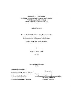
algorithms over a modified version of the graph. The only other change is the difference in the way length is defined over the modified graph, which will allow it to seamlessly translate back to the original graph. The modified graph will take each node and edge in the source graph and convert them to nodes, delineated by different type markers. Then, if two nodes are connected via a particular edge on the source graph, edges will be added to the modified graph to link the corresponding entities.
Figure 4: Source graph converted to modified graph
The definition of the length of a path on the source graph discovered via an algorithm operating on the modified graph can become confusing. Therefore, we will define the length of a path so that the distance between two entities on the source graph is unambiguous. The base condition, or a length of zero, is defined to occur when there are two adjacent entities (node followed by an edge or edge followed by a node). Iterations of the node and edge pairs after the base condition will add one to the path length. Paths with the same endpoint types (From node to node or From edge to edge) This scenario is straightforward. The base condition, or a length of zero, is a single node or single edge. Each subsequent node or edge, depending on the starting type, adds one to the length of the path.
26
Figure 5: Examples of length = 1
Paths with different endpoint types (From node to edge or From edge to node) In this scenario, the base condition of length zero is defined as two adjacent entities: either a node and an edge or an edge and a node. Each subsequent pair of adjacent entities adds one to the length of the path. Node A
Edge B
Edge B
Node C
Length = 0
Length = 0
Figure 6: Examples of the base condition
Figure 7: Examples of lengths of paths starting at nodes and ending at edges
Figure 8: Examples of lengths of paths starting at edges and ending at nodes
4.4 Satisfiability An interesting feature of the path querying system is the path restrictions. For path queries, each path can have a restriction; giving multiple path restrictions if the query contains multiple hops. There are three defined restrictions: a length restriction, an inclusion restriction, and an exclusion restriction. The length restriction specifies a minimum and maximum length for the path. The inclusion restriction specifies zero or more entities that must be part of the path. The exclusion restriction specifies zero or more entities that cannot be part of the path. Some of these restrictions can become
27
inconsistent with themselves, such as specifying a minimum length that is greater than the maximum length. However, inconsistencies can occur more innocently and frequently; especially with the existence of multiple path restrictions when specifying a multi-hop query. To formalize these inconsistencies, we start with a formal definition of the multi-hop path query, followed by a listing of the inconsistencies that can occur. Definitions for a k-hop query (k ≥ 1) From Æ From To Æ To1 Length at least L1,min and at most L1,max Including: I1 = {I1,1, I1,2, I1,3, ...} Excluding: E1 = {E1,1, E1,2, ...} To Æ To2 Length at least L2,min and at most L2,max Including: I2 = {I2,1, I2,2, I2,3, ...} Excluding: E2 = {E2,1, E2,2, ...} etc… Length at least LP,min and at most LP,max Including: IP = {IP,1, IP,2, IP,3, ...} Excluding: EP = {EP,1, EP,2, ...}
N = {From} U {Toi i = 1, 2, K, k } ⎧k = 1, 1; ⎫ r=⎨ ⎬ ⎩k > 1, P, 1, 2, K, k ⎭ Figure 9: Multi-hop Path Query Definition
4.4.1 Individual Length Restrictions
In each restriction r, the minimum and maximum lengths must be non-negative. These two lengths translate into a range that specifies the values for the length of the particular segment. Since a range is being specified, the given minimum length cannot exceed the given maximum length. Any specification where the minimum length was greater than the maximum length would be invalid. To verify that this inconsistency does not exist in the query, the following must be true for each restriction r:
(L
r , min
≤ Lr ,max ) ∧ (Lr ,min ≥ 0) ∧ (Lr ,max ≥ 0)
28
4.4.2 Segment Length Restriction with the Overall Path Length Restriction
After checking for the individual length inconsistency, we can then assume that all of the individual lengths are valid with respect to themselves. However, when specifying a multi-hop query (when k > 1), it is possible that when combining the individual segments’ length ranges to create a total path length range, this range call fall completely outside of the overall path length range. In other words, each of the segments linked together make the path, so the sum of their length ranges (Lk) must fall somewhere in the range of the overall path’s length range (Lp) in order to be valid. Consider the following path that contains three hops: starting from node A and traveling to nodes B, C, and D.
(L A
P , min
C
B
(L
1, min
, L1,max
) (L
)
, LP ,max
2 , min
, L2,max
D
) (L
3, min
, L3,max
)
Given these length restrictions, the total path length must fall within both the path length restriction LP and the summation of the individual segment lengths, as shown below: k
k
i =1
i =1
LK ,min = ∑ Li ,min and LK ,max = ∑ Li ,max
In order for the total path length to fall within both length restrictions LP and LK, these two length ranges must intersect at some point, which potentially defines a more restricted length range over the entire path (LP). This intersection of the two length ranges, L, can be defined as follows:
29
k ⎛ k ⎛ ⎞ ⎞ Lmin = max⎜ ∑ Li ,min , LP ,min ⎟ and Lmax = min⎜ LP ,max , ∑ Li ,max ⎟ i =1 ⎝ i =1 ⎝ ⎠ ⎠
If either of the range’s maximum lengths is less than the other range’s minimum length, then the length restrictions given in the query are invalid, since they provide no valid intersecting length restriction that can apply to the entire path. k ⎛ k ⎛ ⎞ ⎞ ⎜ ∑ Li ,min > LP ,max ⎟ or ⎜ LP ,min > ∑ Li ,max ⎟ i =1 ⎝ i =1 ⎝ ⎠ ⎠
Therefore, to verify that this inconsistency does not exist, the following must be true: ⎧k = 1, ⎪ ⎨ ⎪k > 1, ⎩
true; ⎛ k ⎞ ⎛ ⎜ ∑ Li ,min ≤ LP ,max ⎟ ∧ ⎜ LP ,min ⎝ i =1 ⎠ ⎝
⎫ ⎪ k ⎞⎬ ≤ ∑ Li ,max ⎟⎪ i =1 ⎠⎭
4.4.3 Zero Length Restrictions
For this restriction, we must consider the paths or segments that are defined by the query to have a length equal to zero. In other words, for a particular restriction r,
Lr ,min = Lr ,max = 0 For the remainder of this section, we will refer to both paths and segments as paths since each segment is a miniature path and this particular restriction applies to both objects. A path can start and end with either the same type (node or edge) of node or different types. If the path starts and ends with the same type of node, the from node and to node must be the same node. This is due to the definition of length from Section 4.3: A path of length zero that starts and ends with the same type of node is a single node.
30
If the path starts and ends with different types of nodes, the from node and the to node will be separate nodes by definition (the nodes are of different types). Note that for paths that start and end with the same node type, a path length of zero dictates that the from and to nodes of this path must be the same node, whereas this restriction does not appear in paths that start and end with different node types. If a zerolength path is defined that both starts and ends with the same node type, but the from node and to node are different nodes, then this will never return any paths. Therefore, to verify that this inconsistency does not exist, the following must be true:
(From ∧ ((To
Type
≠ To1,Type ) ∨ (From = To1 ) ∨ (0 < L1,min ≤ L1,max )
i −1,Type
≠ Toi ,Type ) ∨ (Toi −1 = Toi ) ∨ (0 < Li ,min ≤ Li ,max ) i = 2, 3, K , k )
Note that by checking for the inconsistency in each hop, we are also checking indirectly over the entire path, therefore negating the need to specifically check the overall path. 4.4.4 Individual Inclusion and Exclusion Restrictions
In each restriction r, the user will be able to select one or more entities in each of the inclusion and exclusion sets. Within the same restriction, these two sets must be disjoint. It would be invalid for a user to both include and exclude an entity in the same restriction. To verify that this inconsistency does not exist, the following must be true for each restriction r: I r I E r = 0/
4.4.5 From or To Node Conflicts with Exclusion Restrictions
In addition to the individual inclusion and exclusion inconsistency, there is a chance that the overall path’s exclusion restriction (EP) could be inconsistent with the
31
from or to nodes, defined in the set of nodes N. The overall path exclusion set EP cannot contain any of the nodes in N because it would be invalid since the nodes in N are already included by virtue of being the endpoints of the paths. Therefore, since a node cannot be both included and excluded, the two sets EP and N must be disjoint. Also, in a multi-hop query, each segment starts with the To node that preceded the segment. In other words, for all segments i = 2, 3, … k, that segment starts from Toi-1 and ends with Toi. Note that for segment i = 1, that segment starts with From and ends with To1. If any of these segment restriction’s exclusion sets contain their endpoints, this is also invalid. To verify that this inconsistency does not exist, the following must be true: E P I N = 0/ ∧ (Toi ∉ Ei i = 1, 2, K, k ) ∧ (Toi −1 ∉ Ei i = 2, 3, K, k ) ∧ From ∉ E1
4.4.6
Segment
Inclusion/Exclusion
Restrictions
with
the
Overall
Path
Inclusion/Exclusion Restriction
Another conflict occurs concerning the overall path exclusion restriction when a node is contained both within the overall path exclusion set and one or more of the segments’ inclusion sets. It is invalid for a node to be excluded from the entire path (per the overall path exclusion set EP) yet appear in a segment (per the individual segment’s inclusion set Ii, i = 1, 2, …, k). Note that this inconsistency is not reversible. It is possible for a node to be specified for inclusion per the set IP and specified for non-inclusion in a particular segment Ei, i = 1, 2, …, k. This would cause the node to appear in one of the segments that did not specify the node in its exclusion set. Therefore, the overall path exclusion set EP must be disjoint from the union of the segments’ inclusion sets Ii, i = 1, 2, …, k. To verify that this inconsistency does not exist, the following must be true:
32
⎛ k ⎞ E P I ⎜⎜ U I i ⎟⎟ = 0/ ⎝ i =1 ⎠ It would also be possible for every segment to specify a particular node in their exclusion sets while the overall path restriction could specify that node in its inclusion set IP. When the node appears in the set IP, it must appear in at least one segment. However, when every segment specifies the node in their exclusion sets, it is not possible for the node to appear in any of the segments, causing the inconsistency. Therefore, the overall path inclusion set IP must be disjoint from the intersection of the segments’ exclusion sets Ei, i = 1, 2, …, k. To verify that this inconsistency does not exist, the following must be true: ⎛ k ⎞ I P I ⎜⎜ I Ei ⎟⎟ = 0/ ⎝ i =1 ⎠ Note that the reverse of this case is also true. Each segment could specify an entity in their inclusion sets while the overall path restriction could specify the entity in its exclusion set. Note that to check for this described inconsistency, we would need to verify the following: ⎛ k ⎞ E P I ⎜⎜ I I i ⎟⎟ = 0/ ⎝ i =1 ⎠ However, we have already covered this case. This is because of the following property: ⎛ k ⎞ ⎛ k ⎞ ⎜⎜ I I i ⎟⎟ ⊆ ⎜⎜ U I i ⎟⎟ ⎝ i =1 ⎠ ⎝ i =1 ⎠ Therefore, since we already check the same condition as above with a superset of the intersection, we do not need to check for this case specifically.
33
4.5 Interface
To construct the queries, we define several nodes in the Advanced Query Interface system in a hierarchical fashion. See these examples that show the path queries and how they integrate with the AQI:
Figure 10: Example Neighborhood Query
Figure 11: Example Path Query
34
As shown above, it should be straightforward for our users to adapt to using the path queries in the context of the Advanced Query Interface. For the PathCase system, when choosing the root node, the user has the option of picking either the metabolic network graph or the pathway links graph. The query nodes change slightly between graphs, depending on the semantic meaning of the nodes and edges. However, the main idea is still the same. The first portion of each query is the subgraph definition. In our system, this consists of two separate graph restrictions. The first is a flag indicating whether or not the user wishes to include common molecules in the graph. If not, these nodes will be removed from the graph and perhaps some edges that only linked these removed nodes. The second is an option to restrict the graph based on a well-defined subgraph within the graph. See the PathCase graph definitions in Chapter 1 for more details on these subgraphs. Also in this section, a user can choose to have the algorithm operate on a directed (downstream), reverse directed (upstream), or undirected version of these graphs. The neighborhood query continues with a definition of its starting entity, either a node or edge on the graph, and its path restrictions. Note that we are only implementing the length and exclusion restrictions for the neighborhood query for our naïve algorithm, so these are the only options displayed to the user at this time. For more information on this design decision, see the Naïve algorithm section of the next chapter. The path query continues with a definition of its starting entity, either a node or edge on the graph. Then, it continues with one or more definitions of ending entities, again either nodes or edges on the graph. Each of these entities is an interface node in itself that gives both a specification of that node in the graph and a set of path restrictions
35
for that segment. Lastly, the path queries end with a set of path restrictions that pertain to the overall path. After submitting a neighborhood or path query to the AQI, the interface checks for any invalid query specifications. If any invalid specifications are found, a description of the invalid specification and instructions on fixing the query are returned to the user. A comprehensive listing is given below: •
Not specifying exactly one ‘from’ node
•
Not specifying any ‘to’ nodes
•
Empty node, edge, or subgraph name fields
•
Specifying any node, edge, or subgraph name that does not exist in the graph
•
Any nodes in the query’s XML document that should exist but are missing, such as the common molecules specification
•
Any nodes in the query’s XML document that contain invalid values, such as Boolean flags containing values other than ‘true’ or ‘false’
•
Any invalid XML in the query document that does not conform to the schema specified in Appendix 1
4.6 Architecture and Design
Since we used the Advanced Query Interface, we only needed to develop a querying engine for the path queries. This architecture focuses on using a plug-and-play approach to each query, neighborhood and path, where different algorithms can be used by the engine while keeping the same interface of parameter and result passing in and out of the engine. We achieve this by using interfaces for the basic parts of the graph and
36
algorithm, allowing each project to implement its own specific versions of each according to the algorithms they wish to use.
Figure 12: Architecture of the generic Nodes and Edges, with example implementations
Figure 13: Architecture of the generic Graphs, with example implementations
The graph objects consist of nodes and edges. However, the method in which the graphs manipulate these nodes and edges can be changed in whatever fashion is necessary, such as between an adjacency list representation and an adjacency matrix representation.
Figure 14: Architecture of the generic Queries, with example implementations
37
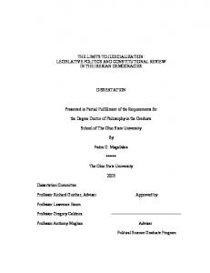
«interface» IQueryParameters +VerifySatisfiability() : void
QueryPathParameters QueryNeighborhoodParameters +minLength : int +maxLength : int +fromNode : INode +includedNodes : List +excludedNodes : List +maxResultLimit : int +maxGraphLimit : int +timeoutLimit : int
+fromNode : INode +toNodes : List +minLength : int +maxLength : int +includedNodes : List +excludedNodes : List +maxResultLimit : int +maxGraphLimit : int +timeoutLimit : int
QueryPathParametersToNode +node : INode +minLength : int +maxLength : int +includedNodes : List +excludedNodes : List
Figure 15: Architecture of the generic Query Arguments, with example implementations
QueryNeighborhoodResults
«interface» IQueryResults
+Nodes : List +Parameters : QueryNeighborhoodParameters +LimitReached : bool +TimeoutReached : bool +DisplayGraph : bool +HiddenGraphText : string +Distance(in node : INode) : int +Distances(out minDistance : int, out maxDistance : int) : void +GetNodes(in type : NodeType, in distance : int) : List QueryPathResults +Paths : List +Parameters : QueryPathParameters +LimitReached : bool +TimeoutReached : bool +DisplayGraph : bool +HiddenGraphText : string +Length(in path : List) : int +Lengths(out minLength : int, out maxLength : int) : void +GetPaths(in length : int) : List +UniqueNodes(in nodeType : NodeType) : List
Figure 16: Architecture of the generic Query Results, with example implementations
The queries are built using three separate interfaces. There is an interface that is responsible for containing the query algorithm’s logic and actually executing the query. This execution occurs on a set of parameters and the execution returns a set of results.
38
Each query algorithm uses its own implementation of parameters and results, which have the option of being shared among multiple querying algorithms. The interface will read in and parse the query, create and initialize a set of parameters for the query, create a new instance of the query, execute the query, and display the results to the user. Also note that we decided that the query should operate on an instance of a graph that is loaded into memory from the database. Of course, the graph implementation could be set up to load the graph as it is accessed. However, this would become difficult and use many expensive I/O operations. For our PathCase implementation, we chose to create the graphs once and cache them in memory. Since we are using a web-based service which would lose the graph as soon as an HTTP request was fulfilled, we chose to use an always-on Windows service to cache our graphs and our queries. The first time a user specifies a graph, we give it a unique name, load the graph into a new instance of IGraph, and send this graph to the service. Once given to the service, the web application can always refer to it via its unique name. Similarly, we can also initialize new instances of queries and send these to the service for caching. This way, we can pass on the name of the graph, the name of the query, and our parameters, and receive a set of results. The communication between the service and the web application occurs by using the .NET framework’s remoting functionality over an interprocess communication (IPC) channel. The formula to create the unique name for each graph is as follows: PathCase_{$AppSetting}_{$GraphName}_{$Restrictions}_{$CommonMolecules}_{$GraphImpl}
The AppSetting variable is used to differentiate between the different versions of the PathCase application running on the same machine. The GraphName variable is used to
differentiate
between
the
different 39
graphs
used
by
our
system:
either
“Metabolic_Network_Graph” or “Pathway_Links_Graph”. The Restrictions variable is a concatenation of all of the id/name pairs for the restrictions given to the graph in a sorted order. The CommonMolecules variable differentiates graphs that use and do not use common molecules. Lastly, the GraphImpl variable differentiates between the use of different implementations of the IGraph interface. For PathCase, we are sticking to using a simple adjacency list implementation since our graphs are sparse. However, if we decide in the future to switch some of the graphs to a different IGraph implementation, this process will be a lot easier since the graph names can remain unique. 4.7 Naïve Algorithm
The naïve algorithm uses a basic depth-first search algorithm to discover the requested paths. In our PathCase implementation, the algorithm also contains the ability to stop the query when a particular timeout limit or maximum results limit is reached. However, we will restrain our discussion here to the depth-first algorithm. PATHQUERY(graph, edgeType, minLength, maxLength, fromNode, toNodes, includedNodes, excludedNodes) 1 Initialize a new list containing lists of paths for each hop: hops 2 fromNode Æ sourceNode 3 foreach toNode in toNodes 4 Initialize a new list of paths for this hop: hop 5 Initialize a new list for this path: path; and add the first node to it, sourceNode 6 toNode.Node Æ destinationNode 7
edgeType, MAX(minLength, toNode.MinLength), DFS(graph, MIN(maxLength, toNode.MaxLength), sourceNode, destinationNode, toNode.IncludedNodes, toNode.ExcludedNodes, sourceNode, 0, path, hop)
8 9
Add hop to hops destinationNode Æ sourceNode
10 Initialize a new list containing the concatenate paths: pathResults 11 hops[0] Æ pathResults 12 for i = 1 to hops.Count – 1
40
13
Initialize a new list of paths: hopPaths
14 15 16 17 18 19 20
foreach pathStart in pathResults foreach pathNextHop in hops[i] Initialize a new temporary list to contain the concatenated path: pathNew Set pathNew equal to pathStart Remove the last step in pathNew Add pathNextHop’s steps to pathNew Add pathNew to hopPaths
21
hopPaths Æ pathResults
22 Initialize a new list containing the final paths: pathResultsFinal 23 foreach path in pathResults 24 if minLength ≤ LENGTH(path) and LENGTH(path) ≤ maxLength 25 continue 26 27
if path does not contain all of the nodes in includedNodes continue
28 29
if path contains any of the nodes in excludedNodes continue
30 Add path to pathResultsFinal 31 return pathResultsFinal edgeType, minLength, maxLength, fromNode, toNode, DFS(graph, includedNodes, excludedNodes, currentNode, currentPathLength, path, results) 32 if minLength ≤ currentPathLength and currentPathLength ≤ maxLength 33 true Æ lengthRestriction 34 if path contains all of the nodes in includedNodes 35 true Æ inclusionRestriction 36 if path does not contain all of the nodes in excludedNodes 37 true Æ exclusionRestriction 38 if currentNode = toNode 39 true Æ destinationRestriction 40 if lengthRestriction, inclusionRestriction, exclusionRestriction, and destinationRestriction are all true 41 Add path to the results list 42 foreach adjacent node adjNode from currentNode in the graph 43 if fromNode.Type = adjNode.Type 44 currentPathLength + 1 Æ adjNodeLength 45 else 46 currentPathLength + 1 Æ adjNodeLength 47 48
if adjNodeLength > maxLength continue
49
if adjNode is a member of path
41
50
continue
51
Push adjNode on to the end of the path list
52
DFS(graph, edgeType, minLength, maxLength, fromNode, toNode, includedNodes, excludedNodes, adjNode, adjNodeLength, path, results)
53
Pop adjNode off of the end of the path list
LENGTH(path) 54 0 Æ length 55 path[0] Æ fromNode 56 for i = 1 to path.Count – 1 57 if fromNode.Type = path[i].Type 58 length + 1 Æ length 59 return length Figure 17: Naïve Path Query Algorithm
The algorithm starts with the PATHQUERY method. This method is responsible for gathering the list of paths for each hop, given by the DFS method, concatenating all of the potential paths, and performing restriction checking on the concatenated paths. In lines 3 – 9, each hop is run through the DFS method and the results, a list of paths, are stored as an element in the hops list. Note the first hop starts with the from node and ends with the first to node. The second hop starts with the first to node and ends with the second to node. This continues for the remainder of the to nodes. Lines 10 – 11 initialize a container for the concatenated paths and initialize it to the list of the first hop’s paths. Each successive iteration of the loop in lines 12 – 21 performs a cross product between the currently concatenated paths and the next hop’s paths. For example, the first time through this loop, the concatenated paths consist of the first hop’s paths and the second hop’s paths are concatenated to them. Forming somewhat of a cross product of paths, each path in the second hop is appended to the end of each path in the first hop. Therefore, if there are two paths in the first hop and three paths in the second hop, there would be a total of six paths after concatenation. The loop would
42
then execute on the concatenated paths (the first and second hops) and the third hop. This achieves a flat listing of all of the possible paths going through each hop. Of course, with several hops, this cross product can grow very quickly. In lines 22 – 30, the overall path restrictions are enforced on the concatenated paths, verifying a proper length, properly included nodes, and properly excluded nodes. Any concatenated path not satisfying these restrictions is removed from the results set before it is returned. To fetch a list of paths between two nodes, a single hop, the DFS method is used by the PATHQUERY method. The DFS method is the heart of the searching algorithm which contains all of the depth-first searching logic. It uses recursion for each step of its traversal and tracks the currently traversed path in the path variable. The currentNode variable contains the node currently being traversed. Lines 32 – 40 check the current path to see if it satisfies the proper length, included nodes, excluded nodes, and endpoint. If so, it is added to the running list of results (the results variable) in line 41. Lines 42 – 53 loop for each adjacent node to the current node. The adjacent node’s path length is computed in lines 43 – 46. If the adjacent node’s length would make the path too long (lines 47 – 48) or the adjacent node has already been traversed (lines 49 – 50), then the algorithm will not recurse on this adjacent node. Otherwise, the node is pushed onto the end of the path in line 51, the recursion call takes place in line 52, and the node is popped back off of the path in line 53. Lastly, there is an auxiliary function used by the PATHQUERY method titled LENGTH that calculates the length of a path given the list of nodes. For any path, the
43
length is equivalent to the number of times the starting entity’s type (node or edge) is repeated throughout the path without including the starting entity.
44
Chapter 5 – Neighborhood Queries
In addition to path queries, we have chosen to add a second type of path query: the neighborhood query. This query is somewhat similar to its path query counterpart in the way that it discovers paths using the same set of path restrictions (length, included and excluded nodes). However, neighborhood queries aren’t designed around returning paths and are instead used to return the entities that are within a well defined vicinity of a particular node. This means that there is no endpoint, only a length that limits the neighborhood to a particular size. Also, this query suits itself towards a breadth-first, rather than depth-first, searching algorithm, which is covered in section 5.3. These differences give the motivation for offering neighborhood queries as a second and distinct type of query from the traditional path queries. In this chapter, we will discuss the differences between the path query covered in Chapter 4 and the neighborhood query. 5.1 Satisfiability
Similarly to the path restrictions, we are also defining path restrictions for the neighborhood queries. Neighborhood queries will only contain one set of path restrictions, since there are not multiple hops involved with these queries. For these queries, we are defining the same three restrictions as the path queries: a length restriction, an inclusion restriction, and an exclusion restriction. Similarly to the path queries, the length restriction specifies a minimum and maximum length for the path, the inclusion restriction specifies zero or more entities that must be part of the path leading out to nodes in the neighborhood, and the exclusion restriction specifies zero or more entities that cannot be part of the path leading out to nodes in the neighborhood. Note that we
45
have chosen not to implement for the inclusion restriction for reasons that we will discuss in the Naïve Algorithm section of this chapter. However, when discussing the neighborhood queries in general, we will be eventually hoping to include this restriction, so we will continue to discuss it here as if we are currently using it. To formalize these inconsistencies, we start with a formal definition of the neighborhood query, followed by a listing of the inconsistencies that can occur. From Æ From Length at least Lmin and at most Lmax Including: I = {I1, I2, I3, ...} Excluding: E = {E1, E2, ...}
Figure 18: Neighborhood Query Definition
5.1.1 Individual Length Restriction
This inconsistency remains from the path queries. The minimum and maximum lengths of the neighborhood must be non-negative since they translate into a range that specifies the values for the size of the neighborhood. Since a range is being specified, the given minimum length cannot exceed the given maximum length. To verify that this inconsistency does not exist in the query, the following must be true:
(Lmin
≤ Lmax ) ∧ (Lmin ≥ 0) ∧ (Lmax ≥ 0)
5.1.2 Individual Inclusion and Exclusion Restrictions
Also similar to the path queries, the user will be able to select one or more entities in each of the inclusion and exclusion sets. These two sets must be disjoint since it would be inconsistent for a user to both include and exclude an entity. To verify that this inconsistency does not exist, the following must be true: I I E = 0/
46
5.1.3 From Node Conflicts with Exclusion Restrictions
There is a possibility that the exclusion restriction (E) could be inconsistent with the from node. The overall path exclusion set E cannot contain the from node because the from node is already included by virtue of being an endpoint of all of the paths to the neighborhood nodes. Therefore, since a node cannot be both included and excluded, the from node cannot be a member of the set E. From ∉ E
5.2 Naïve Algorithm
The naïve algorithm uses a basic breadth-first search algorithm to discover the neighborhood around the starting entity. In our PathCase implementation, the algorithm also contains the ability to stop the query when a particular timeout limit or maximum results limit is reached. However, we will restrain our discussion here to the breadth-first algorithm. BFS(graph, edgeType, minLength, maxLength, fromNode, excludedNodes) 1 Initialize two new lists: visited and results 2 Initialize two new queues: nodes and distances 3 Add fromNode to the nodes queue 4 Add 0 to the distances queue 5 while there are still items in the nodes queue 6 nodes.DEQUEUE() Æ currentNode 7 distances.DEQUEUE() Æ currentDistance 8
Add currentNode to the visited list
9 10
if minLength ≤ currentDistance and currentDistance ≤ maxLength Add the pair of currentNode and currentDistance to the results list
11 12 13 14 15
foreach adjacent node adjNode from currentNode in the graph if fromNode.Type = adjNode.Type currentDistance + 1 Æ adjNodeDistance else currentDistance Æ adjNodeDistance
16
if adjNodeDistance > maxLength
47
17
continue
18 19
if adjNode is a member of visited, nodes, or excludedNodes continue
20 21
Add adjNode to the nodes queue Add adjNodeDistance to the distances queue Figure 19: Naïve Neighborhood Query Algorithm
The breadth-first search algorithm starts with the starting entity and branches out one step at a time by finding the adjacent nodes to the current node in the main loop. The algorithm will stop once the maximum length is surpassed or the adjacent nodes run out, whichever comes first. Note that it is easy to enforce the exclusion restriction in this algorithm by not allowing the traversal of any of the excluded nodes. The converse is not the same for the enforcement of the inclusion restriction. To ensure that a node happens in a path, the information about the path must be kept with each adjacent node. However, the spirit of breadth-first search does not allow for keeping the path information easily. The depthfirst search allows for this with more ease, since it is the nature of the depth-first algorithm to track the current path’s information while traversing a graph. Since the neighborhood algorithm is breadth-first by nature and a depth-first implementation would slow it down considerably, it was determined to sacrifice the inclusion restriction for the naïve implementation of the neighborhood query. Also note another interesting argument for using a depth-first algorithm that can easily track the path information. Consider the following graph:
48
3 2
4
1
5 6 Figure 20: Example Graph
In this graph, there are two distinct paths from node 1 to node 3 without looping through the cycle involving nodes 3, 4, and 5: {1, 2, 3} and {1, 6, 5, 3}. Due to the existence of these two distinct paths, node 3 can be considered to be in the 2neighborhood and the 3-neighborhood of node 1. However, it is difficult to keep the proper path information to allow for node 3 to be in these separate neighborhoods by using a breadth-first algorithm, as discussed above. Therefore, instead of using a costly depth-first algorithm that tracks all of this information, we instead opted for tracking the first time the node is discovered in the breadth-first algorithm. By the nature of the breadth-first algorithm, node 3 from the above example will be first discovered within the 2-neighborhood of node 1, since this is the shortest path from node 1 to node 3. Therefore, node 3 will be included in the 2neighborhood and no other neighborhoods.
49
Chapter 6 – Experimental Results
In this section, we will discuss the performance and scalability of the path querying system that we have been describing in Chapters 4 and 5. We ran our experiments on a client machine with a 2.00 GHz Pentium 4 processor and 1 GB of RAM. Our databases were hosted on separate servers connected to the same LAN as the client using SQL Server 2005. We used two sets of our PathCase data from two separate servers, both with a 3.00 GHz Xeon processor and 16 GB of RAM. Our PathCase system uses two separate sets of data. The first set is termed the ‘Sample’ dataset. This set consists of pathway data that has been manually entered into the system using textbooks and other references. The second set is termed the ‘KEGG’ dataset. This set of data is downloaded from the Kyoto Encyclopedia of Genes and Genomes or KEGG website (http://www.genome.ad.jp/kegg) which makes its data available for free for academic users. We will present several experimental results over the next few sections. We first describe our graph data in terms of its size and the time it takes to load these graphs in to memory for use by our algorithms. Next, we show the performance of the old built-in path queries with the new advanced path queries. Finally, we will discuss the scalability of our path queries in terms of the time it takes to execute our new path queries versus the size of the queries. We will also include the number of results versus the size of the queries. These experiments will show how our algorithms perform as our graph sizes and path lengths increase.
50
Note that for timing experiments, the query timing is only as specific as every 15 milliseconds. If a query’s execution time was in between 0 and 15 milliseconds, it is registered as a time of 0. We have chosen not to include any experiments about the semi-structured AQI queries. This is because the SQL generation algorithm executes very swiftly on a relatively small amount of data when converting the AQI queries into SQL. Therefore, almost all of the query’s processing time is dependent on the database or file structure that is hosting the semi-structured data. Therefore, it seemed that running these experiments would only serve to show the reader how quickly our database server was performing. 6.1 Graph Loading
In our system, we are using two separate graphs: the metabolic network graph, which is a larger and more detailed graph concerning molecules and their reactions (processes); and the pathway links graph, which is a smaller and less detailed graph concerning the big picture of the pathways and their relationships via molecules. For more information on these graphs, see Section 1.1. To help users weed out some potentially unnecessary results in their queries, we offer the option to omit certain molecules from the graph that are so called common molecules, such as water or oxygen. These molecules tend to clutter results more than help the user. There are relatively few common molecules: 10 for our sample dataset and 7 for our KEGG dataset. As to be expected, when comparing the same graph with and without the common molecules included, while the common molecules add virtually no
51
extra nodes, the common molecules add a sizable amount of edges to the graphs, thus increasing their density. The sample dataset’s metabolic network graph consists of 1,360 molecules and processes (nodes) and 5,594 relationships between these molecules and processes (edges). Remember that these edges connect substrate molecules to their processes and processes to their product molecules. Only 10 of these molecules are common molecules, but these common molecules account for 1,124 of the 5,594 edges in the graph, or 20.1% of the edges. Also, the sample dataset contains 38 pathways. These pathways are the primary method for dividing the metabolic network graph into meaningful subgraphs. The KEGG dataset’s metabolic network graph consists of 13,031 molecules and processes and 81,980 relationships between these molecules and processes. Only 7 of these molecules are common molecules and these common molecules account for 6,250 of the 81,980 edges in the graph, or 7.6% of the edges. Also, the KEGG dataset contains 136 pathways. The sample dataset’s pathway links graph consists of 128 pathways and shared molecules (nodes) and 501 relationships between these pathways and shared molecules (edges). Remember that these edges are connected from pathways to molecules they produce via any reaction in that pathway and from molecules to pathways that consume that molecule via any reaction in that pathway. Only 8 of the molecules included as shared molecules in this graph are common molecules (out of the 10 in the entire metabolic network). These molecules account for 167 of the 501 edges in the graph, or 33.3% of the edges. Also, the sample dataset contains 5 organisms. These organisms are the primary method for dividing the pathway links graph into meaningful subgraphs.
52
The KEGG dataset’s pathway links graph consists of 550 pathways and shared molecules and 2,023 relationships between these pathways and shared molecules. Only 4 of the molecules included as shared molecules in this graph are common molecules (out of 7 in the entire metabolic network). These molecules account for only 98 of the 2,023 edges in the graph, or 4.8% of the edges. Also, the KEGG dataset contains 213 organisms (that occur on the pathway links graph). The graphs below show the density of our metabolic network and pathway links graphs for each of our datasets on different sized subgraphs. To obtain an even and consistent variety in the graph sizes, we used both single subgraphs (pathways for the metabolic network and organisms for the pathway links) and graphs consisting of multiple subgraphs. 6000 5000
# of Edges
4000 3000 2000 1000 0 0
200
400
600
800
1000
1200
1400
# of Nodes Without Common Molecules
With Common Molecules
Figure 21: Density of the metabolic network graph from the sample dataset
53
1600
90000 80000 70000
# of Edges
60000 50000 40000 30000 20000 10000 0 0
2000
4000
6000
8000
10000
12000
14000
# of Nodes Without Common Molecules
With Common Molecules
Figure 22: Density of the metabolic network graph from the KEGG dataset 600 500
# of Edges
400 300 200 100 0 0
20
40
60
80
100
120
# of Nodes Without Common Molecules
With Common Molecules
Figure 23: Density of the pathway links graph from the sample dataset
54
140
2500
# of Edges
2000
1500
1000
500
0 0
100
200
300
400
500
600
# of Nodes Without Common Molecules
With Common Molecules
Figure 24: Density of the pathway links graph from the KEGG dataset
In our system, we are fetching the graphs when the server is started so that users will have them in-memory to execute queries against. This loading time must be efficient, but it cannot be burdensome. The same is true for the memory usage. Servers have a high-demand placed on their memory, so we will show that our graphs can be loaded quickly and will not take an excess amount of memory for its index structures. For our sample dataset, the entire metabolic network graph takes 364.6 milliseconds to load and uses 870.4 Kb of memory. The entire pathway links graph takes 104.2 milliseconds to load and uses 69.1 Kb of memory. For the KEGG dataset, the entire metabolic network graph takes 30.7 seconds to load and uses 9,794.4 Kb of memory. The entire pathway links graph takes 328 milliseconds to load and uses 301.6 Kb of memory. For the following experiments, we sampled several different graph sizes that users may encounter by using a combination of subgraphs as described in the previous density
55
experiments. For these experiments, we loaded each individual graph five times in a row. We took an average based on the average of the three median data points within each set of five data points for each graph. We have omitted the data for the sample dataset’s graphs below since the KEGG dataset’s graphs have more variation and better explain the time and memory usage. 14 12
Avg. Time (sec)
10 8 6 4 2 0 0
1000
2000
3000
4000
5000
6000
7000
8000
# of Nodes Without Common Molecules
With Common Molecules
Figure 25: Average time to load the metabolic network for the KEGG dataset
56
9000
7000 6000
Avg. Memory (Kb)
5000 4000 3000 2000 1000 0 0
1000
2000
3000
4000
5000
6000
7000
8000
9000
# of Nodes
Figure 26: Memory usage in Kb of both graphs in the KEGG dataset
6.2 Performance
We also ran experiments against the old built-in path queries that were implemented in the PathCase system before the AQI and compared their performance against the new AQI path queries. In the PathCase system, there are two built-in queries that we singled out to test. The first is a path query: Find paths between two molecules in a pathway. Therefore, in the semantics of our new AQI system, we are looking for a single-hop path from a molecule to another molecule with a single pathway graph restriction. We were executing experiments against this old built-in query when it was discovered that there was a critical error in the execution of the old query that caused it to very frequently return incorrect results. The old system could not be repaired quickly, so we chose to skip this query. Note that this was the only old built-in query that was a path query. However, there were several built-in queries that dealt with a neighborhood. Therefore, we chose to experiment against the following built-in query: Molecules within 57
a given number of steps from another molecule in the metabolic network. In the semantics of our new AQI system, we are looking for a neighborhood of a particular molecule with a length equal to the number of ‘steps’, as specified in the built-in query. The old implementation of the built-in query is implemented by using a similar breadth-first search algorithm to find the neighborhood. This implementation loads its graph at query-time, executes the breadth-first algorithm, and releases the graph. We executed both the old built-in query and the new AQI-based query several times, based on each organism in the dataset. For each organism, we picked two different molecules involved in that organism and queried for the neighborhoods of lengths 1 through 5. For each query, we again ran it five times in a row and took the average based on the three median data points of the set of five data points. There was a problem in picking our random molecules. The built-in query uses a graph based on the subgraph that is restricted by the organism and the pathway of the particular molecule. However, several of the random molecules we picked (4 out of 12 in the sample dataset and 222 out of 422 in the KEGG dataset) were not actually part of a pathway that was part of that organism. Therefore, while the molecule was part of the organism subgraph, it occurred outside of the pathway subgraph. Therefore, the data below is filtered based on queries where the random molecules caused one or more results to be returned. Note that for queries that returned zero results, the old query took between 0 and 20.8 milliseconds to execute (13 milliseconds on average) in the sample dataset. The new query took only 0 milliseconds in the KEGG dataset; remember that any query taking less than 15 milliseconds registers as taking 0 milliseconds on our client machine.
58
1600 1400
Avg. Time (ms)
1200 1000 800 600 400 200 0 0
200
400
600
800
1000
1200
# of Nodes Old Query
New Query
Figure 27: Neighborhood Query Performance in terms of graph size on the KEGG dataset for queries that returned results
Our new AQI query performs very quickly on these short neighborhood queries. More specifically, most queries register 0 milliseconds except for a few making the average time to execute queries virtually 0 (0.005 milliseconds). We have more detailed results of our neighborhood query implementation in the next section complete with experimental results. Also notice that the new query is very fast when compared to the old query and that the old query behaves somewhat erratically and is very unpredictable. This is due to the fact that the new query loads its graphs ahead of time and the old query loads its graphs at query-time. Therefore, the old query contains an overhead when compared to the new query. Since the breadth-first neighborhood algorithm is quite faster when compared to the I/O time of loading the graphs, this accounts for the major difference in the query times between the two implementations. The erratic behavior can also be
59
explained by the variations in loading times when fetching data continuously from the database server. The next set of graphs shows the timing of the old and new queries versus both the average execution time and the number of neighborhood results. The number of neighborhood results is a count of the number of nodes within the neighborhood size of the source node. The nodes are both the molecules and processes for the metabolic network graph and both the pathways and shared molecules for the pathway links graph. The general trend of the timing between the old and new query is held in these graphs. However, note that the sample dataset’s queries are returning far more results and are consequently taking longer to execute. This is because the graphs on the sample dataset’s organism subgraphs are larger than the KEGG dataset’s organism subgraphs. Also, there is a striking similarity in the old query for each dataset between the average query time and the number of results. This similarity is due to the fact that the old query, while rendering time was not included, does prepare its results for rendering while computing its neighborhood instead of returning a pure list of results.
60
2000 1800 1600
Avg. Time (ms)
1400 1200 1000 800 600 400 200 0 0
1
2
3
4
5
6
5
6
Neighborhood Size (steps) Old Query
New Query
70
# of Neighborhood Results
60 50 40 30 20 10 0 0
1
2
3
4
Neighborhood Size (steps)
Figure 28: Neighborhood Query Performance in terms of neighborhood size on sample dataset
61
350 300
Avg. Time (ms)
250 200 150 100 50 0 0
1
2
3
4
5
6
5
6
Neighborhood Size (steps) Old Query
New Query
1.6
# of Neighborhood Results
1.4 1.2 1.0 0.8 0.6 0.4 0.2 0.0 0
1
2
3
4
Neighborhood Size (steps)
Figure 29: Neighborhood Query Performance in terms of neighborhood size on KEGG dataset
6.3 Scalability
Lastly, we ran experiments testing the scalability of our new path querying system. For each of the neighborhood and path queries, we executed query based on a random molecule per subgraph from lengths 0 to 20 to determine how the execution time scales as the path lengths are increased.
62
For the neighborhood queries, we executed experiments on both graphs. For the metabolic network graph, we performed queries on built up subgraphs (one pathway, then two pathways, then three, etc.) to get increasingly larger graph sizes. We chose a random molecule for each graph and executed a neighborhood query of sizes 0 through 20. For the pathway links graph, we performed queries on built up subgraphs using organisms to get increasingly larger sizes. We chose a random molecule for each graph and executed queries of sizes 0 through 20. The average times shown in the data below are obtained from five runs for each query, taking the average of the median three data points. 40 35
Avg. Time (ms)
30 25 20 15 10 5 0 0
5
10
15
Neighborhood Size (steps) Metabolic Network
63
Pathway Links
20
25
700
# of Neighborhood Results
600 500 400 300 200 100 0 0
5
10
15
20
25
Neighborhood Size (steps) Metabolic Network
Pathway Links
Figure 30: Neighborhood Query Scalability in terms of neighborhood size on sample dataset 450 400
Avg. Time (ms)
350 300 250 200 150 100 50 0 0
5
10
15
Neighborhood Size (steps) Metabolic Network
64
Pathway Links
20
25
3500
# of Neighborhood Results
3000 2500 2000 1500 1000 500 0 0
5
10
15
20
25
Neighborhood Size (steps) Metabolic Network
Pathway Links
Figure 31: Neighborhood Query Scalability in terms of neighborhood size on KEGG dataset
As shown for the sample dataset, the neighborhood query on the metabolic network graph starts to plateau around size 7. This shows that this graph does not have a radius much larger than 7 steps. The KEGG dataset’s metabolic network also plateaus around step 16. For the pathway links graph in both datasets, the execution time is extremely minimal, since these graphs are quite smaller than their counterparts. Overall, the neighborhood queries are quite speedy and although they experience an exponential growth, the overall execution time remains well under a second once the times plateau. For the path queries, we also executed experiments on both graphs. For the metabolic network graph, we performed queries on built up subgraphs to get increasingly larger graph sizes, similar to the neighborhood scalability experiment. We chose a random pair of molecules for each graph and executed a path query of lengths 0 through 20. For the pathway links graph, we performed queries on the overall graph by picking 10 random pairs of molecules and executing a path query of lengths 0 through 20. The
65
average times shown in the data below are obtained from an average of three runs per query. 70000 60000
Avg. Time (ms)
50000 40000 30000 20000 10000 0 0
5
10
15
20
25
20
25
Path Length Metabolic Network
Pathway Links
1600 1400 1200
# of Paths
1000 800 600 400 200 0 0
5
10
15 Path Length
Metabolic Network
Pathway Links
Figure 32: Path Query Scalability in terms of path length on sample dataset
In the metabolic network graph of the sample dataset, there is a high exponential growth with respect to time after length 5. The curve then plateaus after length 14. This plateau is due to a timeout limit we enforced on these experiments of two minutes. In 66
other random experimentation, longer length path queries were executing much longer than five minutes, showing that the exponential growth continues after length 14. This also accounts for the spikes in the number of paths, including the large one that occurs around length 12. As the queries timeout more frequently, only those queries with a smaller number of paths are finishing in time, causing this graph to be skewed. See the following graph for a summary of the amount of queries that experience a timeout for the metabolic network. 250
# of Queries
200
150
100
50
0 0
1
2
3
4
5
6
7
8
9
10 11 12 13 14 15 16 17 18 19 20
Path Length Completed
Timed Out
Figure 33: The number of path queries that experience a timeout in the metabolic network graph of the sample dataset
However, for the pathway links graph in the sample dataset, which is quite smaller than the metabolic network, these queries took no longer than one second to complete and 136 milliseconds on average. They also returned no paths, since it is quite rare that a set of random molecules is actually connected due to this graph’s low density. However, since the new query performs the same search when no results are returned
67
versus when results are returned, queries that do contain results should not take much longer. 90000 80000
Avg. Time (ms)
70000 60000 50000 40000 30000 20000 10000 0 0
5
10
15
20
25
20
25
Path Length Metabolic Network
Pathway Links
250
# of Paths
200
150
100
50
0 0
5
10
15 Path Length
Metabolic Network
Pathway Links
Figure 34: Path Query Scalability in terms of path length on KEGG dataset
In the metabolic network graph of the KEGG dataset, there is a similar high exponential growth with respect to time after length 3. The curve plateaus towards the latter quarter of the graph, again due to the two minute timeout restriction we enforced on 68
these experiments. The timeout restriction also creates the low points in the results with respect to the number of paths. See the following graph for a summary of the amount of queries that experience a timeout for the metabolic network. 900 800 700
# of Queries
600 500 400 300 200 100 0 0
1
2
3
4
5
6
7
8
9
10 11 12 13 14 15 16 17 18 19 20
Path Length Completed
Timed Out
Figure 35: The number of path queries that experience a timeout in the metabolic network graph of the KEGG dataset
Again, the pathway links graph took at most 1.1 seconds to complete and 260 milliseconds on average. There are an average of 0.2 paths returned, with 80% of the queries returning no paths and 20% of the queries finding a single path. To address the problem of exponential growth in the future, we can leverage our existing framework, which performs well for neighborhood queries, and implement a new algorithm for path queries.
69
Chapter 7 – Conclusion
In this thesis, we have proposed a simple and powerful Advanced Querying Interface (AQI) that uses a single unified interface to support queries against both semistructured and graph data. While it was originally created solely for semi-structured data, the hierarchical tree-like structure of the query construction interface lends itself to support other types of queries, like those against graph data. We therefore developed and implemented a new interface for the AQI which is backwards-compatible with the semistructured capabilities, but allows for the addition of any type of query that can be expressed within the confines of the interface. In the future, the AQI could be extended to support negation, variables, or self-joins (as described in [New2004]). One other bonus about our new framework is the XML query documents that are passed between the interface and the querying engine. In the future, the AQI could be used by other applications that can use this XML format or queries could be loaded and saved by the system for future use. We have also developed and implemented a path querying library to support our path queries that the AQI generates. Using this library, the graph data and querying algorithms are designed to be completely separate entities that communicate with each other via basic common interfaces and can be used in a plug-and-play type manner. We chose to implement basic breadth-first and depth-first search algorithms for our queries, which perform fairly well. However, as shown in the larger path queries, we will need to implement another algorithm that can outperform a basic depth-first traversal. Also within our path querying framework, we have developed a set of path restrictions that can be applied to a path within our queries so that users can drill down to
70
the exact results they are looking for. These restrictions not only include a range of lengths but also two sets of nodes that must be included or excluded from a path. The use of the path restrictions may limit the use of pre-existing traversing algorithms and may require the creation of a new algorithm that is focused on indexing the paths as well as their restrictions.
71
Appendix 1 – AQI Query XML Document Schema
72
Bibliography
[BZ2005]
Stanislav Bartoň and Pavel Zezula. ρ-index – An Index for Graph Structured Data. 2005.
[CHMW1996]
Michael Carey, Laura Haas, Vivek Maganty, and John Williams. PESTO: An Integrated Query/Browser for Object Databases. VLDB, p. 203 – 214, 1996.
[Dog2006]
U. Dogrusoz, E. Z. Erson, E. Giral, E. Demir, O. Babur, A. Cetintas, and R. Colak. PATIKAweb: a Web interface for analyzing biological pathways through advanced querying and visualization. Bioinformatics Vol. 22 No. 3 p. 374 – 375 2006.
[Kri2002]
L. Krishnamurthy, J. Nadeau, G. Özsoyoğlu, M. Özsoyoğlu, G. Schaeffer, M. Tasan, and W. Xu. Pathways database system: an integrated system for biological pathways. Bioinformatics Vol. 19 No. 8 p. 930 – 937 2003.
[Les2005]
Ulf Leser. A Query Language for Biological Networks. Bioinformatics Vol. 21 Suppl. 2 p. ii33 – ii39 2005.
[New2004]
Scott W. Newman. A Tree-Structured Interface for Querying Semi-Structured Data. M.S. Thesis 2004.
[NO2004]
Scott Newman, Z. Meral Özsoyoğlu. A Tree-Structured Query Interface for Querying Semi-Structured Data. SSDBM, 2004.
[ONOT2004]
Z. M. Özsoyoğlu, J. Nadeau, G. Özsoyoğlu, M. Tasan. Towards an Integrated Software System for Biological Pathways. IEEE Data Eng. Bull. 27(4): 53-60, 2004.
[TL2007]
Silke Trißl and Ulf Leser. Fast and Practical Indexing and Querying of Very Large Graphs. SIGMOD, p. 845 – 856, 2007.
[Wang2006]
Haixun Wang, Hao He, Jun Yang, Philip S. Yu, and Jeffrey Xu Yu. Dual Labeling: Answering Graph Reachability Queries in Constant Time. ICDE, p. 75, 2006.
[Zlo1977]
M. Zloof. Query by Example. IBM Systems Journal p. 324 – 343 No. 4 1977.
73