most business-related disciplines, as well as the social and health sciences. .... coefficients generated by nonlinear multivariate analysis software tools such as ...
Advanced mediating effects tests, multi-group analyses, and measurement model assessments in PLS-based SEM Ned Kock
Full reference: Kock, N. (2014). Advanced mediating effects tests, multi-group analyses, and measurement model assessments in PLS-based SEM. International Journal of e-Collaboration, 10(1), 1-13.
Abstract Use of the partial least squares (PLS) method has been on the rise among e-collaboration researchers. It has also seen increasing use in a wide variety of fields of research. This includes most business-related disciplines, as well as the social and health sciences. The use of the PLS method has been primarily in the context of PLS-based structural equation modeling (SEM). This article discusses a variety of advanced PLS-based SEM uses of critical coefficients such as standard errors, effect sizes, loadings, cross-loadings and weights. Among these uses are advanced mediating effects tests, comprehensive multi-group analyses, and measurement model assessments.
KEYWORDS: Multivariate Statistics, Partial Least Squares, Structural Equation Modeling, WarpPLS, Mediating Effects, Multi-group Analyses
1
Introduction The partial least squares (PLS) method has been increasingly used by e-collaboration researchers, as well as by researchers in related fields, such as information systems. It also has seen increasing use in most business-related areas of investigation, as well as in fields of research related to the social and health sciences. This is particularly the case in the context of PLS-based structural equation modeling (SEM). This article discusses a variety of advanced tests used in PLS-based SEM, with a focus on tests that employ the following coefficients: standard errors, effect sizes, loadings, crossloadings, and weights. The discussion presented here builds on the software WarpPLS, version 4.0 (Kock, 2013). The extensive set of outputs generated by this software makes it particularly useful in the illustration of the tests discussed (Kock, 2010; 2011a; 2011b), and allows for a straightforward discussion of the different steps involved in those tests. As it will be clear in the following sections, the approach taken in this article is very hands-on. This article is aimed at practitioners who need to conduct multivariate analyses as part of their research, analyses that can sometimes be very complex and difficult to conduct, potentially creating a new source of errors. Hopefully this article will make their work somewhat easier, as well as less time-consuming and prone to errors, serving as a handy reference that they can go to whenever they need to conduct advanced mediating effects tests, comprehensive multi-group analyses, and measurement model assessments.
Using standard errors and effect sizes for path coefficients Standard errors and effect sizes for path coefficients are provided by WarpPLS in two tables where one standard error and effect size is provided for each path coefficient (see Figure 1). The effect sizes are analogous to Cohen’s (1988) f-squared coefficients, but calculated through a novel procedure (described below). Standard errors and effect sizes are provided in the same order as the path coefficients, so that users can easily visualize them; and, in certain cases, use them to perform additional analyses. Standard errors and effect sizes are provided for “normal” latent variables, as well as for latent variables associated with moderating effects, which are essentially interaction latent variables. These are indicated in column and row names as products between latent variables. For example, the cell whose row is “Effe” and whose column is “Proc*Effi” refers to the moderating effect of the latent variable “Proc” on the link between “Effi” and “Effe”. The effect sizes are calculated as the absolute values of the individual contributions of the corresponding predictor latent variables to the R-square coefficients of the criterion latent variable in each latent variable block. Unlike Cohen’s (1988) formula for estimation of effect sizes in multiple regression, which has a correction term in its denominator, WarpPLS calculates the exact values of the individual contributions of the corresponding predictor latent variables to the R-square coefficients of the criterion latent variable they point at. It does so by “freezing” parameters in successive calculations with the predictors included and excluded, leading to exact results and thus obviating the need for corrections. With the effect sizes users can ascertain whether the effects indicated by path coefficients are small, medium, or large. The values usually recommended are 0.02, 0.15, and 0.35; respectively (Cohen, 1988). Values below 0.02 suggest effects that are too weak to be considered relevant 2
from a practical point of view, even when the corresponding P values are statistically significant; a situation that may occur with large sample sizes. Figure 1. Standard errors and effect sizes for path coefficients window
Use in tests of mediating effects One of the additional types of analyses that may be conducted with standard errors are tests of the significance of mediating effects using the approach discussed by Preacher & Hayes (2004), for linear relationships; and Hayes & Preacher (2010), for nonlinear relationships. The latter, discussed by Hayes & Preacher (2010), assumes that nonlinear relationships are force-modeled as linear; which means that the equivalent test using WarpPLS would use warped coefficients with the earlier linear approach discussed by Preacher & Hayes (2004). The classic approach used for testing mediating effects is the one discussed by Baron & Kenny (1986), which does not rely on standard errors. The mediating effect significance test approach that employs standard errors for path coefficients is as follows. As discussed below, it applies to both linear and nonlinear path coefficients generated by nonlinear multivariate analysis software tools such as WarpPLS. Let us assume that we have two latent variables, X and Y, and that we want to test whether another latent variable M is a significant mediator of the relationship between X and Y. One would normally build the following two models to conduct this test, and calculate all of the path coefficients and P values. The first model would be a simple one, with only two variables and one link: 𝑋 → 𝑌. The second model would be a more complex one, with three variables and three links: 𝑋 → 𝑌 and 𝑋 → 𝑀 → 𝑌. As a first step, the test entails calculating the path coefficients and corresponding P values in the first simple model and in the second more complex model, as well as the related standard errors in the second model. Let us assume that the path coefficient in the first simple model (𝑋 → 𝑌) is 𝑟. Since this is a model with only two variables, the path coefficient 𝑟 is also the bivariate correlation between the two variables. The path coefficients in the second model are referred to as follows: 𝑎 for the 𝑋 → 𝑀 link, 𝑏 for the 𝑀 → 𝑌 link, and 𝑐 for the 𝑋 → 𝑌 link. 3
We then need to calculate a modified standard error for the product 𝑎 ∙ 𝑏, sometimes referred to as Sobel’s standard error, using the equation below. Next we calculate the critical ratio: 𝑇�� = (𝑎 ∙ 𝑏)⁄𝑆�� . This ratio is then used to calculate the P value associated with the product of coefficients 𝑎 ∙ 𝑏. 𝑆�� = �𝑏 � ∙ 𝑆� � + 𝑎� ∙ 𝑆� � + 𝑆� � ∙ 𝑆� �
In practice one does not need to build the first simple model with WarpPLS, as the software automatically generates all of the bivariate correlations among latent variables. All one has to do is to get 𝑟 from the latent variable correlations table generated by WarpPLS. Also, at the time of this writing, a spreadsheet was available from www.warppls.com to automate the calculation of Sobel’s standard error, the product of path coefficients, as well as the critical ratios and P values discussed here. For a mediating effect to be considered significant, the P value associated with the product of coefficients 𝑎 ∙ 𝑏 must be significant at a specified level (usually lower than .05). Additionally, the P values associated with 𝑎, 𝑏, and 𝑟 must also be significant. If these conditions are met, and the P value associated with 𝑐 is not significant, we can say that full mediation is occurring. If the P value associated with 𝑐 is significant, we can say that partial mediation is occurring. It may be advisable, particularly in nonlinear analyses, to employ a variation of this test, which would entail using the total effect coefficient between X and Y, instead of 𝑟. The reason is that it is possible that 𝑟 will be low because two nonlinear effects will “cancel each other out” in a cross-sectional analysis, but yet will still be associated with a strong lagged effect (e.g., associated with a time lag). This strong lagged effect will be better captured through the use of the total effect coefficient between X and Y than with 𝑟; the latter may in some cases artificially suggest no effect. An alternative approach to the analysis of mediating effects, which is arguably much less time-consuming and prone to error than the approaches mentioned above, would be to rely on the estimation of indirect effects. These indirect effects and related P values are automatically calculated by WarpPLS, and allow for the test of multiple mediating effects at once, including effects with more than one mediating variable. Use in multi-group analyses Another type of analysis that can employ standard errors for path coefficients is what is often referred to as a multi-group analysis. One of the main goals of this type of analysis is to compare pairs of path coefficients for identical models but based on different samples. An example would be the analysis of the same model but with data collected in two different countries. This is usually done by first calculating a pooled standard error (𝑆�� ) for each of the path coefficient pairs in the two models (see, e.g., Keil et al., 2000), using the equation below. In this equation, 𝑁� is the sample size for the first model, 𝑁� is the sample size for the second model, 𝑆� is the standard error for the path coefficient in the first model, and 𝑆� is the standard error for the path coefficient in the second model. (�� ��)�
𝑆�� = ��(�
� ��� ��)
(�� ��)�
∙ 𝑆� � + (�
� ��� ��)
∙ 𝑆� � � ∙ ��
�
��
+
�
��
� 4
The equation above assumes that the standard errors 𝑆� and 𝑆� are not significantly different from one another. That is, it assumes that the absolute difference between those standard errors is indistinguishable from zero; an assumption that is frequently met. If this assumption is violated, 𝑆�� should be calculated based on a different equation. Using this different equation, shown below, is often referred to as employing the Satterthwaite method. The Satterthwaite method is arguably more generic, but apparently less widely used. It also relies on a simpler equation, as can be seen below. Perhaps the reason why it is less widely used is that it frequently yields slightly higher values for 𝑆�� than the pooled standard error method; the differences are usually very small though. 𝑆�� = �𝑆� � + 𝑆� �
Following the calculation of 𝑆�� , we then calculate the critical ratio: 𝑇�� = (𝛽� − 𝛽� )⁄𝑆�� . Here (𝛽� − 𝛽� ) is the difference between the path coefficients in the first and second models. This ratio (𝑇�� ) is then used to calculate the P value associated with the difference between the path coefficients. At the time of this writing, a spreadsheet was available from www.warppls.com to automate the calculation of the pooled and Satterthwaite standard errors, the critical ratios, and the associated P values. The procedure just discussed focuses on path coefficients, which are structural model coefficients. This procedure should also be employed with weights. While with path coefficients researchers may be interested in finding statistically significant differences, with weights the opposite is typically the case – they will want to ensure that differences are not statistically significant. The reason is that significant differences between path coefficients can be artificially caused by significant differences between weights in different models. Such differences may result from a form of common method bias due to questionnaire translation problems. This is a nontrivial issue in multi-group studies where data is collected in different countries with different languages and cultures. Common method bias can be tested based on full collinearity VIFs (Kock & Lynn, 2012), but only for a given sample. With two separate samples from different countries, for example, common method bias could go unnoticed and significantly bias the results of a multi-group analysis. Let us assume that a study used of the same questionnaire in two different countries, where the questionnaire was translated from one language to another. The translation may have led to a change in meaning for some question-statements, which would be reflected in different weights. These different weights could then artificially inflate differences between path coefficients, suggesting between-country differences. To rule out this possibility, one needs to ensure equivalence of measurement models, which would be indicated by equivalent weights, before structural model elements such as paths are compared. Here P values are expected to be greater, as opposed to lower, than a certain threshold. The recommended threshold is .10 for a conservative test. That is, P values should be greater than .10 for the conclusion that no significant differences exist. This threshold of .10 is twice the .05 threshold used to ascertain that a significant difference exists. Both are based on one-tailed tests. A more relaxed approach would be to employ the same threshold of .05 for the tests involving both path coefficients and weights.
5
Some would argue that loadings should be used as well in measurement model equivalence tests, in addition to weights, but in practice using loadings in addition to weights in these tests seems to lead to redundant results.
Using combined loadings and cross-loadings Combined loadings and cross-loadings are provided by WarpPLS in a table with each cell referring to an indicator-latent variable link (see Figure 2). Latent variable names are listed at the top of each column, and indicator names at the beginning of each row. In this table, the loadings are from a structure matrix (i.e., unrotated), and the cross-loadings from a pattern matrix (i.e., rotated). Figure 2. Combined loadings and cross-loadings window
As with other coefficients discussed earlier, indicator loadings and cross-loadings are provided for “normal” latent variables, as well as for latent variables associated with moderating effects. These are indicated in column and row names as products between latent variables and indicators, respectively. For example, the column “Proc*Effi” refers to an interaction latent variable, which itself is associated with one or more moderating effects of the latent variable “Proc” on the link or links between “Effi” and one or more latent variables. Since loadings are from a structure matrix, and unrotated, they are always within the -1 to 1 range. This obviates the need for a normalization procedure to avoid the presence of loadings whose absolute values are greater than 1. The expectation here is that loadings, which are shown within parentheses, will be high; and cross-loadings will be low. WarpPLS uses the PLS regression algorithm as its default (Kock, 2012). This algorithm does not allow the structural (a.k.a. inner) model to influence the measurement (a.k.a. outer) model, which tends to minimize collinearity and avoid other problems. A property of PLS regression is that, when only two indicators are used in one latent variable, their unrotated loadings are reported as being the same. This is not an indication of a problem, but the repetition in the table sometimes causes confusion among users of the software.
6
Kaiser normalization can be employed to avoid these repeated values (this should be done automatically by the software starting in version 4.0 of WarpPLS). Through a Kaiser normalization, each row of a table of loadings and cross-loadings is divided by the square root of its communality. This has the effect of making the sum of squared values in each row add up to 1. P values are also provided for indicator loadings associated with all latent variables. These P values are often referred to as validation parameters of a confirmatory factor analysis, since they result from a test of a model where the relationships between indicators and latent variables are defined beforehand. Conversely, in an exploratory factor analysis, relationships between indicators and latent variables are not defined beforehand, but inferred based on the results of a factor extraction algorithm. The principal components analysis algorithm is one of the most popular of these algorithms, even though it is often classified as being outside the scope of classical factor analysis. Contrary to popular belief, PLS-based SEM is not a component-based form of SEM; at least not in the sense of principal components analysis. Often one sees researchers refer to PLS-based SEM as an analysis method that has two main stages: a principal components analysis, whereby weights and loadings are calculated; and a path analysis. This is incorrect. PLS-based SEM has two main stages: a PLS regression analysis, whereby weights and loadings are calculated; and a path analysis. Instead of PLS regression, variations known as PLS modes may be employed, but not a principal components analysis. For research reports, users will typically use the table of combined loadings and cross-loadings provided by WarpPLS when describing the convergent validity of their measurement instrument. A measurement instrument has good convergent validity if the question-statements (or other measures) associated with each latent variable are understood by the respondents in the same way as they were intended by the designers of the question-statements. In this respect, two criteria are recommended as the basis for concluding that a measurement model has acceptable convergent validity: that the P values associated with the loadings be lower than 0.05; and that the loadings themselves be equal to or greater than 0.5 (Hair et al., 1987; 2009). Indicators for which these criteria are not satisfied may be considered for removal or reassignment to other latent variables. These criteria do not apply to formative latent variable indicators, which are assessed in part based on P values associated with indicator weights. If the offending indicators are part of a moderating effect, then you should consider removing the moderating effect if it does not meet the requirements for formative measurement (discussed later). As previously noted, moderating effect latent variable names are displayed on the table as product latent variables (e.g., “Effi*Proc”). Also as noted earlier, moderating effect indicator names are displayed on the table as product indicators (e.g., “Effi1*Proc1”). High P values for moderating effects, to the point of being nonsignificant at the 0.05 level, may suggest multicollinearity problems; which can be further checked based on the latent variable coefficients generated by WarpPLS, more specifically, the full collinearity variance inflation factors (VIFs). Some degree of collinearity is to be expected with moderating effects, since the corresponding product variables are likely to be correlated with at least their component latent variables. Moreover, moderating effects add nonlinearity to models, which can in some cases compound
7
multicollinearity problems. Because of these and other related issues, moderating links should be included in models with caution. Standard errors are also provided for the loadings, in the column indicated as “SE”, for indicators associated with all latent variables. They can be used in specialized tests. Among other purposes, these standard errors can be used in multi-group analyses, with the same model but different subsamples, to ascertain measurement model equivalence. However, as mentioned earlier, if measurement model equivalence is tested based on weights, then testing it using loadings may be redundant.
Using pattern loadings and cross-loadings Pattern loadings and cross-loadings are provided by WarpPLS in a table with each cell referring to an indicator-latent variable link (see Figure 3). Latent variable names are listed at the top of each column, and indicator names at the beginning of each row. In this table, both the loadings and cross-loadings are from a pattern matrix (i.e., rotated). Figure 3. Pattern loadings and cross-loadings window
Since these loadings and cross-loadings are from a pattern matrix, they are obtained after the transformation of a structure matrix through a widely used oblique rotation frequently referred to as Promax. The structure matrix contains the Pearson correlations between indicators and latent variables, which are not particularly meaningful prior to rotation in the context of measurement instrument validation. Rotated loadings and cross-loadings are particularly useful in the visual identification by users of mismatches between indicators and latent variables. Such mismatches are usually associated with low loadings and high cross-loadings. Because an oblique rotation is employed, in some cases loadings may be higher than 1 (Rencher, 1998). This could be a hint that two or more latent variables are collinear, although this may not necessarily be the case; better measures of collinearity among latent variables are the full collinearity VIFs reported by WarpPLS with other latent variable coefficients. 8
The main difference between oblique and orthogonal rotation methods is that the former assume that there are correlations, some of which may be strong, among latent variables. A case can easily be made in favor of oblique rotation methods in SEM analyses, because by definition latent variables are expected to be correlated. Without correlations among latent variables, no path coefficient would be significant. Technically speaking, it is possible that a research study would hypothesize only neutral relationships between latent variables, but one does not usually find published examples of research studies where this happens.
Using structure loadings and cross-loadings Structure loadings and cross-loadings are provided by WarpPLS in a table with each cell referring to an indicator-latent variable link (see Figure 4). Latent variable names are listed at the top of each column, and indicator names at the beginning of each row. In this table, both the loadings and cross-loadings are from a structure matrix (i.e., unrotated). Often these are the only loadings and cross-loadings provided by other PLS-based SEM software tools. Figure 4. Structure loadings and cross-loadings window
As the structure matrix contains the Pearson correlations between indicators and latent variables, this matrix is not particularly meaningful or useful prior to rotation in the context of collinearity or measurement instrument validation. Here the unrotated cross-loadings tend to be fairly high, even when the measurement instrument passes widely used validity and reliability test criteria. Still, some researchers recommend using this table as well to assess convergent validity, by following two criteria: that the cross-loadings be lower than 0.5; and that the loadings be equal to or greater than 0.5 (Hair et al., 1987; 2009). Note that the loadings here are the same as those provided in the combined loadings and cross-loadings table. The cross-loadings, however, are different.
9
Using indicator weights Indicator weights are provided by WarpPLS in a table, much in the same way as indicator loadings are (see Figure 5). All cross-weights are zero, because of the way they are calculated through PLS regression. Each latent variable score is calculated as an exactly linear combination of its indicators, where the weights are multiple regression coefficients linking the indicators to the latent variable. Figure 5. Indicator weights window
P values are provided for weights associated with all latent variables. These values can also be seen, together with the P values for loadings, as the result of a confirmatory factor analysis. In research reports, users may want to report these P values as an indication that formative latent variable measurement items were properly constructed. This also applies to moderating latent variables that pass criteria for formative measurement, when those variables do not pass criteria for reflective measurement. As in multiple regression analysis (Miller & Wichern, 1977; Mueller, 1996), it is recommended that weights with P values lower than 0.05 be considered valid items in a formative latent variable measurement item subset. Formative latent variable indicators whose weights do not satisfy this criterion may be considered for removal. The reference to multiple regression made here is due to the fact that the weights linking indicators to their latent variables, at the measurement model level, are equivalent to the standardized partial regression coefficients linking independent to dependent variables in a typical multiple regression model. The same can generally be said with respect to the path coefficients in individual latent variable blocks. There are indeed many parallels between PLSbased SEM and multiple regression analyses. With the P values provided for weights, users can also check whether moderating latent variables satisfy validity and reliability criteria for formative measurement, if they do not satisfy criteria for reflective measurement. This can help users demonstrate validity and reliability in hierarchical analyses involving moderating effects, where double, triple etc. moderating effects are tested. For instance, moderating latent variables can be created, added to the model as standardized indicators, and then their effects modeled as being moderated by other latent variables; an example of double moderation.
10
In addition to P values, VIFs are also provided for the indicators of all latent variables, including moderating latent variables. These can be used for indicator redundancy assessment. In reflective latent variables indicators are expected to be redundant. This is not the case with formative latent variables. In formative latent variables indicators are expected to measure different facets of the same construct, which means that they should not be redundant. The VIF threshold of 3.3 has been recommended in the context of PLS-based SEM in discussions of formative latent variable measurement (Cenfetelli & Bassellier, 2009; Petter et al., 2007). A rule of thumb rooted in the use of WarpPLS for many SEM analyses in the past suggests an even more conservative approach: that capping VIFs to 2.5 for indicators used in formative measurement leads to improved stability of estimates. The multivariate analysis literature, however, tends to gravitate toward higher VIF thresholds, such as 5 and 10. One of the reasons for this is that this literature tends to refer to directly measured variables, not latent variables; particularly not latent variables resulting from collinearity minimization algorithms such as PLS regression. In models with latent variables measured through single indicators, which are not “true” latent variables, the use of higher VIF thresholds may well be justified. Also, capping VIFs at 2.5 or 3.3 may in some cases severely limit the number of possible indicators available. Given this, it is recommended that VIFs be capped at 2.5 or 3.3 if this does not lead to a major reduction in the number of indicators available to measure formative latent variables. One example would be the removal of only 2 indicators out of 16 by the use of this rule of thumb. Otherwise, the criteria below should be employed. Two criteria, one more conservative and one more relaxed, are recommended by the multivariate analysis literature in connection with VIFs in this type of context. More conservatively, it is recommended that VIFs be lower than 5; a more relaxed criterion is that they be lower than 10 (Hair et al., 1987; 2009; Kline, 1998). High VIFs usually occur for pairs of indicators in formative latent variables, and suggest that the indicators measure the same facet of a formative construct. This calls for the removal of one of the indicators from the set of indicators used for the formative latent variable measurement. These criteria are generally consistent with formative latent variable theory (see, e.g., Diamantopoulos, 1999; Diamantopoulos & Winklhofer, 2001; Diamantopoulos & Siguaw, 2006). Among other characteristics, formative latent variables are expected, often by design, to have many indicators. Yet, given the nature of PLS regression and related algorithms, indicator weights will normally go down as the number of indicators go up, as long as those indicators are somewhat correlated, and thus P values will normally go up as well. Moreover, as more indicators are used to measure a formative latent variable, the likelihood that one or more will be redundant increases. This will be reflected in high VIFs. As with indicator loadings, standard errors are also provided here for the weights, in the column indicated as “SE”, for indicators associated with all latent variables. These standard errors can be used in specialized tests. Among other purposes, they can be used in multi-group analyses, with the same model but different subsamples. As discussed earlier, here users may want to compare the measurement models to ascertain equivalence, using a multi-group comparison technique such as the one discussed earlier, and thus ensure that any observed between-group differences in structural model coefficients, particularly in path coefficients, are not due to measurement model differences.
11
Discussion and conclusion The PLS method has been increasingly used by e-collaboration researchers, as well as by researchers in other fields. This has been particularly true in the context of SEM, although it has also been the case in more basic tests such as variations of ANOVA, ANCOVA, MANOVA, MANCOVA, multiple regression, and path analysis. Conceptually, these more basic tests can all be seen as special cases of SEM. This article discussed a variety of tests that are routinely used in the context of PLS-based SEM, and that can also be selectively used in more basic tests. The focus of the discussion is on tests that employ critical coefficients such as standard errors, effect sizes, loadings, crossloadings and weights. Several recommendations were made here. With the effect sizes users can ascertain whether the effects indicated by path coefficients are small, medium, or large. The values usually recommended are 0.02, 0.15, and 0.35; respectively. Standard errors can be used in advanced tests of mediating effects and multi-group analyses. Loadings and cross-loadings can be used in various tests, particularly validity tests. This applies to rotated and unrotated loadings and cross-loadings. It also applies to loadings and cross-loadings obtained with or without Kaiser normalization adjustments. As loadings and cross-loadings can be used in various tests, so can weights, particularly in the context of formative latent variable measurement. With respect to multi-group analyses, one key issue must be highlighted. The procedure discussed here in connection with path coefficients should also be employed with weights. The reason is that differences between path coefficients can be caused by differences between weights in different models. Therefore, one needs to ensure that the models are equivalent with respect to their measurement, which would be indicated by non-significant differences in weights, before structural coefficients (e.g., path coefficients) are compared. The approach taken in this article is very applied, with illustrations based on the software WarpPLS that were aimed to be as clear and straightforward as possible. The article is aimed at practitioners who need to conduct multivariate analyses as part of their research investigations. These analyses can sometimes be very complex, difficult, and time-consuming. Hopefully this article will make the work of these applied researchers a little easier.
Acknowledgments The author is the developer of the software WarpPLS, which has over 5,000 users in 33 different countries at the time of this writing, and moderator of the PLS-SEM e-mail distribution list. He is grateful to those users, and to the members of the PLS-SEM e-mail distribution list, for questions, comments, and discussions on topics related to the use of WarpPLS.
References Cenfetelli, R., & Bassellier, G. (2009). Interpretation of formative measurement in information systems research. MIS Quarterly, 33(4), 689-708. Cohen, J. (1988). Statistical power analysis for the behavioral sciences. Hillsdale, NJ: Lawrence Erlbaum. 12
Diamantopoulos, A. (1999). Export performance measurement: Reflective versus formative indicators. International Marketing Review, 16(6), 444-457. Diamantopoulos, A., & Siguaw, J.A. (2006). Formative versus reflective indicators in organizational measure development: A comparison and empirical illustration. British Journal of Management, 17(4), 263–282. Diamantopoulos, A., & Winklhofer, H. (2001). Index construction with formative indicators: An alternative scale development. Journal of Marketing Research, 37(1), 269-177. Hair, J.F., Black, W.C., Babin, B.J., & Anderson, R.E. (2009). Multivariate data analysis. Upper Saddle River, NJ: Prentice Hall. Hayes, A. F., & Preacher, K. J. (2010). Quantifying and testing indirect effects in simple mediation models when the constituent paths are nonlinear. Multivariate Behavioral Research, 45(4), 627-660. Keil, M., Tan, B.C., Wei, K.-K., Saarinen, T., Tuunainen, V., & Wassenaar, A. (2000). A crosscultural study on escalation of commitment behavior in software projects. MIS Quarterly, 24(2), 299–325. Kline, R.B. (1998). Principles and practice of structural equation modeling. New York, NY: The Guilford Press. Kock, N. (2010). Using WarpPLS in e-collaboration studies: An overview of five main analysis steps. International Journal of e-Collaboration, 6(4), 1-11. Kock, N. (2011a). Using WarpPLS in e-collaboration studies: Descriptive statistics, settings, and key analysis results. International Journal of e-Collaboration, 7(2), 1-17. Kock, N. (2011b). Using WarpPLS in e-collaboration studies: Mediating effects, control and second order variables, and algorithm choices. International Journal of e-Collaboration, 7(3), 1-14. Kock, N. (2013). WarpPLS 4.0 User Manual. Laredo, Texas: ScriptWarp Systems. Kock, N., & Lynn, G.S. (2012). Lateral collinearity and misleading results in variance-based SEM: An illustration and recommendations. Journal of the Association for Information Systems, 13(7), 546-580. Miller, R.B., & Wichern, D.W. (1977). Intermediate business statistics: Analysis of variance, regression and time series. New York, NY: Holt, Rihehart and Winston. Mueller, R.O. (1996). Basic principles of structural equation modeling. New York, NY: Springer. Petter, S., Straub, D., & Rai, A. (2007). Specifying formative constructs in information systems research. MIS Quarterly, 31(4), 623-656. Preacher, K.J., & Hayes, A.F. (2004). SPSS and SAS procedures for estimating indirect effects in simple mediation models. Behavior Research Methods, Instruments, & Computers, 36 (4), 717-731. Rencher, A.C. (1998). Multivariate statistical inference and applications. New York, NY: John Wiley & Sons.
13