Advanced solution methods in topology optimization

Advanced solution methods in topology optimization and shape sensitivity analysis Manolis Papadrakakis and Yiannis Tsompanakis

Advanced solution methods 57

Institute of Structural Analysis and Seismic Research, National Technical University of Athens, Greece

Ernest Hinton and Johann Sienz University of Wales, Swansea, Wales, UK Introduction In recent years, the integration of topology and shape optimization methods with the modern CAD technology has made remarkable progress in achieving automatically optimum designs. Topology optimization is usually employed first, in order to avoid local optima due to a crude initial layout, followed by shape optimization in order to fine tune the optimum layout. Communication between the two optimization stages is carried out through an image processing tool which extracts the final topology and pass the model to the shape optimizer[1]. Integrated methodologies, where topology and shape optimization are dealt not in succession but simultaneously, using the same design model in every optimization step, have also evolved[2,3]. Topology optimization is a tool which assists the designer in the selection of suitable initial structural topologies by removing or redistributing material of the structural domain. The procedure starts with an initial layout of the structure followed by a gradual “removal” of a small portion of low stressed material which is being used inefficiently. This procedure is a typical case of structural reanalysis. which results in small variations of the stiffness matrix between two optimization steps. In a shape optimization problem the aim is to improve a given topology by minimizing an objective function subjected to certain equality and inequality constraints, where all functions are related to the design variables. The shape optimization algorithm proceeds with the following steps: (1) a finite element mesh is generated; (2) displacements and stresses are evaluated; (3) sensitivities are computed by perturbing each design variable by a small amount; and This work has been supported by HC&M 9203390 project of the European Union. The Swansea authors wish to acknowledge funding provided by the EPSRC project GR/K22839.

Engineering Computations, Vol. 13 No. 5 1996, pp. 57-90. © MCB University Press, 0264-4401

EC 13,5

58

(4) the optimization problem is solved and the new shape of the structure is defined. These steps are repeated until convergence has occurred. The most timeconsuming part of a gradient-based optimization process is devoted to the sensitivity analysis phase. For this reason several techniques have been developed for the efficient calculation of the sensitivities in an optimization problem. The semi-analytical and the finite difference techniques are the two most widely used types of sensitivity analysis techniques. In the first case only the right-hand sides change and the coefficient matrix remains the same, while in the second case the coefficient matrix is modified as well due to the perturbations of the design variables. The latter technique results in a similar problem as in the case of topology optimization. Usually, a structural optimization problem, whether it is topology, shape, or an integrated structural optimization problem is a computationally intensive task, where 60 to 90 per cent of the computations are spent on the solution of the finite element equilibrium equations. Although it is widely recognized that hybrid solution methods, based on a combination of direct and iterative solvers, outperform their direct counterparts, both in terms of computing time and storage, little effort has been devoted until now to their implementation in the field of structural optimization. In the present study three innovative solution methods are implemented based on the preconditioned conjugate gradient (PCG) and Lanczos algorithms. The first method is a PCG algorithm with a preconditioner resulted from a complete or an incomplete Cholesky factorization, the second is a PCG algorithm in which a truncated Neumann series expansion is used as preconditioner, and the third is the preconditioned Lanczos algorithm properly modified to treat multiple right-hand sides. The numerical tests presented demonstrate the computational advantages of the proposed methods, which become more pronounced in large-scale and/or computationally-intensive optimization problems. Topological design of stuctures In most shape optimization problems the topology of the structure is given and only the shape of the boundaries varies (boundary variation method). This optimized design, however, is dependent on the given topology and thus this solution may correspond only to a local optimum. For this reason, topology optimization techniques have been developed which allow the designer to optimize the layout or the topology of a structure. Topological or layout optimization can be undertaken by employing one of the following main approaches which have evolved during the last few years[1]: (1) the ground structure[4]; (2) the homogenization method[5]; (3) the bubble method[6]; and (4) the evolutionary fully-stressed design technique[7].

The first three approaches have several things in common. They are optimization techniques with an objective function, design variables, constraints and they solve the optimization problem by using an algorithm based on sequential quadratic programming (approach (1)), or on an optimality criterion concept (approaches (2) and (3)). However, inherently linked with the solution of the optimization problem is the complexity of these approaches. The fully-stressed design technique on the other hand, although not an optimization algorithm in the conventional sense, proceeds by removing inefficient material, and therefore optimizes the use of the remaining material in the structure, in an evolutionary process. The work presented in this study related to topology optimization is based on an improved implementation of the evolutionary fully stressed design technique proposed by Hinton and Sienz[1], and investigates the influence of effective hybrid solution techniques on the overall performance of the topology optimization problem. Basic algorithm for topology optimization This algorithm for topology optimization is based on the simple principle that material which has small stress levels is used inefficiently and therefore it can be removed. Thus, by removing small amounts of material at each optimization step, the layout of the structure evolves gradually. In order to achieve convergence of the whole optimization procedure, it is important for the amount of material removed at each stage to be small and to maintain a smooth transition from one layout of the structure to the subsequent one. The domain of the structure, which is called the reference domain, can be divided into the design domain and the non-design domain. The non-design domain covers regions with stress concentrations, such as supports and areas where loads are applied, and therefore it cannot be modified throughout the whole topology optimization process. After the generation of the finite element mesh, the evolutionary fully stressed design cycle is activated, where a linear elastic finite element stress analysis is carried out. The equivalent stress σeq, or the maximum principal stress σpr, for each element can be computed, which for convenience is called in both cases the stress level and is denoted as σevo. The maximum stress level σmax Of the elements in the structure at the current optimization step is defined, and all elements that fulfil the condition σ evo < ratre * σ max (1) are removed, or switched off, where ratre is the rejection rate[7]. The elements are removed by assigning them a relatively small elastic modulus which is typically E off = 10 –5 * E on .

(2 )

In this way the elements switched-off virtually do not carry any load and their stress levels are accordingly small in subsequent analyses. This strategy is called “hard kill”, since the low stressed elements are immediately removed, in contrast with the “soft kill” method where the elastic modulus varies linearly

Advanced solution methods 59

EC 13,5

60

and the elements are removed more gradually. The remaining elements are considered active and they are sorted in ascending order according to their stress levels before a subsequent analysis is performed. The number of active elements to be switched off per optimization step depends on the following control parameters: (1) the parameter switl related to the minimum percentage of active elements to be switched off providing a lower bound for the number of elements to be switched off; (2) the parameter switu related to the maximum percentage of active elements providing an upper bound for the number of elements to be switched-off; (3) the cut-off stress parameter strmx, which is used to switch off all the elements having stresses lower than the cut-off stress. The first two parameters are expressed as a percentage of the elements to be switched off per optimization step and operate as a safeguard against a stagnation of the evolutionary process, or an abrupt change of the stress field in the remaining structure. When only a few elements are switched off the rejection rate is incremented by the evolution rate in order to accelerate the convergence of the whole process ratrei + 1 = ratrei + ratev (i = 1, 2, …).

(3 )

Typical values for the rejection rate and the evolution rate are ratre = 1 per cent and ratev = 1 per cent. In addition to the above-mentioned control parameters there are two more criteria which influence the switching off of elements: (1) Composite suppression. During the evolutionary process there will sometimes be single elements which are switched on but which are surrounded by elements that are switched off. This may result in a chess board pattern-like topology of elements which are alternatively switched on and off, and it is not desired. (2) Element growth. This option allows the designer to switch on elements adjacent to elements in which the stress level is larger than a specified stress limit. This is the only way in which elements which have been switched off can be switched on again. The iterative process of element removal and addition is continued until one of several specified convergence criteria is met: (1) All stress levels are larger than a certain percentage value, defined by rspst, of the maximum stress. This criterion assumes that a fully stressed design has been achieved and the material is used efficiently. (2) The number of active elements is smaller than a specified percentage, defined by rspel, of the total number of elements.

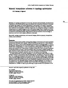
(3) When element growth is allowed the evolutionary process is completed when more elements are switched on than they are switched off. Shape optimization The shape optimization method used in the present study is based on a previous work for treating two-dimensional problems by Hinton and Sienz[8]. It consists of the following essential ingredients: shape generation and control; mesh generation; adaptive finite element analysis; sensitivity analysis; and shape optimization. The method proceeds with the following steps: (1) At the outset of the optimization, the geometry of the structure under investigation has to be defined. The boundaries of the structure are modelled using cubic B-splines which, in turn, are defined by a set of key points. Some of the co-ordinates of these key points will be the design variables which may or may not be independent. (2) An automatic mesh generator is used to create a valid and complete finite element model. A finite element analysis is then carried out and the displacements and stresses are evaluated. An h-type adaptivity analysis may be incorporated in this stage. (3) The sensitivities of the constraints and the objective function to small changes in the design variables are computed either with the finite difference, or the semi-analytical method. (4) A suitable mathematical programming method, like the sequential quadratic programming SQP algorithms, is used to optimize the design variables. If the convergence criteria for the optimization algorithm are satisfied, then the optimum solution has been found and the solution process is terminated, otherwise the new geometry is defined and the whole process is repeated from step (2). The whole procedure is depicted in Figure 1. Sensitivity analysis Sensitivity analysis is the most important and time-consuming part of shape optimization. Although sensitivity analysis is mostly mentioned in the context of structural optimization, it has evolved into a research topic of its own. Several techniques have been developed which can be mainly distinguished by their numerical efficiency and their implementation aspects. The methods for sensitivity analysis can be divided into discrete and variational methods[9]. In the variational approach the starting point is an idealized but continuous structure, such as beam or shell. Applying basic variational theorems to the functions and operators describing the structure and the optimization problem, the sensitivity coefficients can be determined. In this case, the sensitivities are given as boundary and surface integrals which are then solved after the structure has been discretized. In the discrete approach the derivatives or the

Advanced solution methods 61

EC 13,5

Start

Create optimization model

62 Create finite element model

Evaluate new mesh parameters No

Analyse with finite elements

Adaptivity?

Error OK?

Yes

Yes

Estimate error

No

Evaluate sensitivities

Optimize parameters

Update optimization model

No

Figure 1. Flowchart of the shape optimization algorithm

Optimum? Yes

Stop

sensitivities of the characteristic parameters, i.e. displacements, stresses, volume, etc., which define the objective and constraint functions of the discretized structure, are evaluated using the finite element equations. The implementation for discrete methods is simpler than that for variational techniques. A further classification of the discrete methods is as follows: • Global finite difference method. A full finite element analysis has to be performed for each design variable and the accuracy of the method depends strongly on the value of the perturbation of the design variables.

•

•

Semi-analytical method. The stiffness matrix of the initial finite element solution is retained during the computation of the sensitivities. This provides an improved efficiency over the finite difference method by a relatively small increase in the algorithmic complexity. The accuracy problem involved with the numerical differentiation can be overcome by using the exact semi-analytical method, which needs more programming effort than the simple method but, is computationally more efficient. Analytical method. The finite element equations, the objective and constraint functions, are differentiated analytically. The implementation is more complex than for the other two discrete methods and requires access to the source code.

The decision on which method to implement depends strongly on the type of the problem, the structure of the computer program and the access to the source code. The variational method is usually more reliable but requires a more complex computer implementation, whereas when a finite difference method is applied the formulation is much simpler and the sensitivity coefficients can be easily evaluated. In the present investigation the first two variations of discrete approach have been implemented. Irrespective of the type of approach used, the sensitivity analysis can take 50-80 per cent of the total computational effort required to solve the whole optimization problem. Therefore, an efficient and reliable sensitivity analysis module results in a considerable reduction of the overall computational effort. The global finite difference (GFD) method. In shape optimization the stiffness matrix K and the loading vector b are functions of the design variables sk (k = 1, …, n). The primary objective is to compute the derivative of the displacement field with respect to sk. The GFD method provides a simple and straightforward way of computing the sensitivity coefficients. This method requires the solution of a linear system of equations Kx = b, where x is the displacement vector, for the original design variables s0, and for each perturbed design variable spk = s 0k + ∆s k , where ∆s k is the magnitude of the perturbation. The design sensitivities for the displacements ∂x/∂sk and the stresses ∂σ/∂sk are computed using a forward difference scheme:

∂ x / ∂sk ≈ ∂σ / ∂sk ≈

∆x ∆sk ∆σ ∆sk

= =

x( sk + ∆sk ) – x( sk )

(4 )

∆sk

σ ( sk + ∆sk ) – σ ( sk ) ∆sk

.

(5 )

The perturbed displacement vector x(sk + ∆sk) is evaluated by K( sk + ∆sk ) x ( sk + ∆sk ) = b( sk + ∆sk ) and the perturbed stresses σ (sk + ∆sk) are computed from

(6 )

Advanced solution methods 63

EC 13,5

64

σ ( sk + ∆sk ) = DB( sk + ∆sk ) x ( sk + ∆sk )

(7 )

where D and B are the elasticity and the deformation matrices respectively. The GFD scheme is usually sensitive to the accuracy of the computed perturbed displacement vectors, which is dependent on the magnitude of the perturbation. Too small values for the perturbation lead to insignificant changes of the response parameters making the whole procedure vulnerable to round-off errors, whereas too big values give rise to inaccuracies associated with any scheme based on truncated Taylor series expansion. The proper choice for the value of the perturbation is problem dependent and can be found by trial and error. It is usually taken between 10–3 and 10–5. The semi-analytical (SA) method. The SA method is based on the chain rule differentiation of the finite element equations Kx = b ∂x ∂K ∂b K + x= (8 ) ∂sk ∂sk ∂sk which when rearranged results in ∂x K = b*k ∂sk

(9 )

where b*k =

∂b ∂sk

–

∂K ∂sk

(10 )

x

b k* represents a pseudo-load vector. The derivatives ∂b/∂s k and ∂K/∂s k are computed for each design variable by recalculating the new values of K(sk + ∆sk) and b(sk + ∆sk) for a small perturbation ∆sk of the design variable sk, while the stiffness matrix remains unchanged throughout the whole sensitivity analysis. The conventional semi-analytical (CSA) method. In the CSA sensitivity analysis, the values of the derivatives in equation (8) are calculated by applying the forward difference approximation

∂ K / ∂sk ≈ ∂ b / ∂sk ≈

∆K ∆sk ∆ b ∆sk

= =

K( sk + ∆sk ) – K( sk ) ∆sk b( sk + ∆sk ) – b( sk ) ∆sk

.

(11)

(12 )

For maximum efficiency of the semi-analytical method only those elements which are affected by the perturbation of a certain design variable are involved into the calculations of ∂b/∂sk and ∂K/∂sk. Stress gradients can be calculated by differentiating σ = DBx as follows

∂σ

∂D

=

∂sk

Bx + D

∂sk

∂B ∂sk

x + DB

∂x ∂sk

.

(13 )

Advanced solution methods

Since the elasticity matrix, D, is not a function of the design variables then equation (13) reduces to

∂σ

=D

∂sk

∂B

x + DB

∂sk

∂x ∂sk

.

(14 )

In equation (14), ∂x/∂sk may be computed as indicated in equation (4), while the term ∂B/∂sk is computed using a forward finite difference scheme as follows

∂B

∆B

=

∂sk

∆sk

=

B( sk + ∆sk ) – B( sk ) ∆sk

.

(15 )

The “exact” semi-analytical (ESA) method. The CSA method may suffer some drawbacks in particular types of shape optimization problems. This is due to the fact that, in the numerical differentiation of the element stiffness matrix with respect to shape design variables, the components of the pseudo load vector associated with the rigid body rotation do not vanish. A similar inaccuracy problem is not found if the analytical or the global finite difference method is employed. The solution suggested by Olhoff et al.[10] alleviates the problem by performing an “exact” numerical differentiation of the elemental stiffness matrix based on computationally inexpensive first order derivatives. These derivatives can be obtained on the element level as follows

∂k

n

=∑

∂sk

∂k ∂α j

i = 1 ∂α j

(16 )

∂sk

where n is the number of element nodal co-ordinates affected by the perturbation of the design variable sk and αj is the nodal co-ordinate of the element which can be either a x-co-ordinate or a y-co-ordinate. The derivative ∂αj/∂sk can be computed “exactly” by means of a forward difference scheme

∂α j ∂sk

=

∆α j ∆sk

=

α j ( sk + ∆sk ) – α j ( sk ) ∆sk

(17 )

while the derivative ∂k/∂αj is computed by differentiating the element stiffness matrix expression k = ∫ BT DB| J |dΩ Ω

with respect to a perturbation of the nodal co-ordinate αj:

(18 )

65

EC 13,5

66

 ∂B  ∂| J| | J |dΩ + ∫ BT DB = 2 ∫  BT D dΩ   ∂α j ∂α ∂α Lj j Ω Ω

∂k

(19 )

after using symmetry properties of D and k. Equation (19) can be rewritten as ∂k ˆ T DB ˆ ( j ) | J |dΩ = 2∫ B (20 ) ∂α j Ω where Bˆ (j ) is given as ˆ ( j ) = ∂B + 2 B ∂ | J |. B 2 | J | ∂α j ∂α j

(21)

Since equations (18) and (20) have the same structure the existing computer code for calculating the stiffness matrix can be used for the computation of the derivative of the elemental stiffness matrix, as long as it is possible to substitute Bˆ ( j ) in the place of B. The question as to whether ∂k/∂αj can be computed “exactly” is now reduced to an investigation of whether the derivatives of B and |J| with respect to a nodal co-ordinate perturbation αj can be computed with the required accuracy. The derivative ∂|J|/∂αj can be computed “exactly” with a forward difference scheme

∂ | J | ∆ | J | J (α j + ∆α j ) – J (α j ) = = . ∆α j ∆α j ∂α j

(22 )

For the differentiation of B, the derivatives of the shape functions with respect to a change in the nodal co-ordinates need to be evaluated. This can be done “exactly” using the following formula   ∂  N i , x  –1 ∂ | J |  N i , x   =– J   ∂α j  N i , y  ∂α j  N i , y  where ∂J/∂αj can also be computed with a forward difference scheme

∂J ∂α j

=

∆J ∆α j

=

J (α j + ∆α j ) – J (α j ) ∆α j

.

(23 )

(24 )

Applying equation (23) to all terms in the B matrix, the “exact” derivative of ∂B/∂ α j can be evaluated. The evaluation of the “exact” derivatives of the stiffness matrix is computationally more expensive than the corresponding derivatives of the CSA method. This overhead, however, is counterbalanced by the gains in accuracy and the improvement on the overall optimization procedure. The stress sensitivities are computed in the same way as with the CSA method using equation (14), where the term ∂B/∂s k, instead of using

equation (15), is evaluated in this case with respect to the nodal perturbations of co-ordinate αj using equations (23) and (24). Hybrid solution methods The implementation of hybrid solution schemes in structural optimization, which are based on a combination of direct and preconditioned iterative methods, has not yet received the attention it deserves from the research community, even though in finite element linear solution problems and particularly when dealing with large-scale applications their efficiency is well documented. In this work several hybrid methods are applied in the context of topology and shape optimization based on PCG and Lanczos algorithms. The methods are properly modified to address the special features of the particular optimization problems at hand, while mixed precision arithmetic operations are proposed resulting in additional savings in computer storage without affecting the accuracy of the solution. The preconditioned conjugate gradient (PCG) method The PCG method has become very popular for the solution of large-scale finite element problems. An efficient preconditioning matrix makes PCG very attractive even for ill-conditioned problems without destroying the characteristic features of the method. Several global preconditioners have been used in the past for solving finite element linear problems[11]. The most important factor for the success of the hybrid methods is the preconditioning technique used to improve the ellipticity of the coefficient matrix. Preconditioning techniques based on incomplete Cholesky factorization are capable of increasing the convergence rate of the basic iterative method, at the expense of more storage requirements. In the present study the incomplete procedure by magnitude proposed by Bitoulas and Papadrakakis[12], is implemented in a mixed precision arithmetic mode, and a compact storage scheme is used to store both the coefficient and the preconditioning matrices row-by-row. The reason for performing an incomplete factorization is to obtain a reasonably accurate factorization of the coefficient matrix without generating too many fill-ins, whereas a complete factorization produces the strongest possible preconditioner, which in exact precision arithmetic is actually the inverse of K. Both approaches lead to the factorization of the coefficient matrix K: LDLT = K0 + ∆K–E, where E is an error matrix which does not have to be formed. For this class of methods, E is defined by the computed positions of “small” elements in L which do not satisfy a specified magnitude criterion and therefore are discarded. If we have to deal with a reanalysis problem, which is the case of GFD sensitivity analysis and topology optimization problems, the matrix E is taken as the ∆K matrix, whereas in the case of SA sensitivity analysis both E and ∆K are taken as null matrices. Non-zero terms are stored in a real vector, while the corresponding column numbers are stored in an integer vector of equal length. An additional integer

Advanced solution methods 67

EC 13,5

68

vector with length equal to the number of equations is used to record the start of each row inside the compact scheme. Thus, the total storage requirements are NA (stiffness in double precision arithmetic), NL (preconditioner in single precision arithmetic) and NA + NL + 2*(N + 1) short integers (for the addressing), where N is the number of equations. Also the complete Cholesky factorization of the “initial” stiffness matrix K0 is used as the preconditioning matrix in its original skyline form and is stored in single precision arithmetic, thus it does not require the NL short integers for the addressing the compact. Another important factor affecting the performance of the PCG iterative procedure for solving Kx = b is the determination of the residual vector. The accuracy achieved and the computational labour of the method is largely determined by how this is calculated. A study performed in [11] revealed that the computation of the residual vector of the equilibrium equations Kx = b from its defining formula r(m) = Kx(m) – b, with an explicit or a first order differences matrix-vector multiplication Ku(m), offers no improvement in the accuracy of the computed results. In fact, it was found that, contrary to previous recommendations, the calculation of the residuals by the recursive expression r (m+1) = r(m) + αmKd(m), where d is the direction vector, produces a more stable and well-behaved iterative procedure. Based on this observation a mixed precision arithmetic PCG implementation is proposed in which all computations are performed in single precision arithmetic, except for double precision arithmetic computation of the matrix-vector multiplication involved in the recursive evaluation of the residual vector. This implementation is a robust and reliable solution procedure even for handling large and illconditioned problems, while it is also computer storage-effective. It was also demonstrated to be more cost-effective, for the same storage demands, than double precision arithmetic calculations[10,11]. The Neumann-CG method (NCG) The approximation of the inverse of the stiffness matrix using a Neumann series expansion has been used in the framework of stochastic finite element analysis, structural reanalysis and damage analysis problems. In all these cases the method was implemented on an “as is” basis, without any corrections to improve the quality of the solution, thus the results were satisfactory only in the vicinity of the initial design and unacceptable for large modifications of the stiffness matrix. In a recent study by Papadrakakis and Papadopoulos[13] the method was successfully integrated with the conjugate gradient algorithm resulting in a significant improvement on the accuracies achieved with low additional computational cost. It can also handle cases with significant changes of the stiffness matrix. The solution of a typical reanalysis problem ( K0 + ∆K ) x = b yields

(25 )

x = ( I + K0–1∆K )–1 K0–1b.

(26 )

The term in parenthesis can be expressed in a Neumann expansion giving x = ( I – P + P 2 – P 3 + …)K0–1b

(27 )

with P = K0–1 ∆K. The response vector can now be represented by the following series x = x0 – Px0 + P x0 – P x0 + ⋅ ⋅ ⋅

(28 )

x = x0 – = x1 + x2 – x3 + ⋅ ⋅ ⋅

(29 )

2

2

or The series solution can also be expressed by the following recursive equation K0 xi = ∆Kxi – 1 i = 1, 2 , … (30 ) The advantage of this expression is that the stiffness matrix has to be factorized once while the additive terms xi to the solution of equation (29) can be computed by successive backward and forward substitutions. The series may be truncated after a fixed number of terms or according to some error norm given by i

xi /

∑ (– 1)k xk

≤ ε1

(31)

k =0

or ri / b ≤ ε 2

(32 )

where ri = b – (K0 + ∆K)xi. The first criterion is most frequently used since it is computationally more efficient. The second criterion requires the evaluation of the residual vector which involves an additional matrix vector multiplication for each Neumann term. In order to improve the quality of the preconditioning matrix, M, used in the PCG method, a Neumann series expansion is implemented for the calculation of the preconditioned vector z (m) = M –1 r (m) of the PCG algorithm. The preconditioning matrix is now defined as the complete global stiffness matrix K = K 0 + ∆K, but the solution for z is performed approximately using a truncated Neumann series expansion. Thus, the preconditioned vector, z, of the PCG algorithm is obtained at each iteration by (33 ) z = z 0 – z1 + z2 – z3 + ⋅ ⋅ ⋅ z 0 is given by z 0 = K0–1r0

(34 )

and K0 zi = ∆Kzi – 1

i = 1, 2 , …

Advanced solution methods

(35 )

69

EC 13,5

70

The incorporation of the Neumann series expansion in the preconditioned step of the PCG algorithm can be seen from two different perspectives. From the PCG point of view an improvement of the quality of the preconditioning matrix is achieved by computing a better approximation to the solution of x = (K 0 + ∆K)–1b than the one provided by the preconditioning matrix K0. From the Neumann series expansion point of view, the inaccuracy entailed by the truncated series is alleviated by the conjugate gradient iterative procedure. It remains to be seen, however, whether the anticipated improvement on the convergence properties of the PCG method or of the Neumann series expansion implies also a reduction on the overall computational effort by counteracting the additional cost involved at each iteration. The storage requirements for NCG in mixed precision arithmetic are the following: the compact stiffness K is stored in double precision arithmetic and the factorized skyline stiffness and ∆K are stored in single precision arithmetic, while 2*[NA + (N + 1)] + (N + 1) short integers are needed for the addressings. The preconditioned Lanczos method for multiple right-hand sides When a sequence of right-hand sides has to be processed, direct methods possess a clear advantage over the conventional application of iterative methods. The major effort concerned with the factorization of the coefficient matrix is not repeated and only a back and forward substitution is required for each subsequent right-hand side. In the case of iterative methods the whole work has to be repeated from the beginning for every right-hand side. Papadrakakis and Smerou[14] presented a new implementation of the Lanczos algorithm for solving linear systems of equations with a sequence of right-hand sides. This algorithm handles all approximations to the solution vectors simultaneously without the necessity for keeping in fast or secondary storage the tridiagonal matrix or the orthonormal basis produced by the Lanczos method. Thus, when the first solution vector has converged to a required accuracy, good approximations to the remaining solution vectors have simultaneously been obtained. It then takes fewer iterations to reach the final accuracy by working separately on each of the remaining vectors. The equilibrium equations for multiple right-hand sides are stated as follows: K[ x1 … xk ] = [ b1 … b k ]

(36 )

KX = B

(37 )

or and the characteristic equations of the Lanczos algorithm become Tj Yj = Q jT Ro

(38 )

and X j = Q j Yj

(39 )

where Yj = [y1, …, Yk]j, Xj = [x1, …, Xk]j consist of the jth approximation to the k auxiliary and solution vectors y and x respectively, and Ro = [r1o, …, r ko] with roi = bi – Kxoj consists of the residual vectors. By using a Cholesky root-free decomposition of Ti we get Lj D j Z j = Q T j Ro

(39 )

X j = Cj Z j

( 40 )

with Zj = [z1, …, zk] and LjCTj = QTj. The last components of matrix Zj are now given by

ζ ji = (q Tj roi – δ j d j – 1ζ j – 1, i ) / d j

( 41)

and the new approximation to the solution vectors by [ x1 … xk ] j = [ x1 … xk ] j – 1 + c j [ζ jl … ζ jk ].

( 42 )

The algorithm can be stated as follows (where k is the number of right-hand sides, i is the right-hand side counter, j is the iteration counter): Phase I. Initialization r1(1) = b(1) – Kx (o1) For i = 2 , … , k x0( i ) = M –1 [b( i ) – r1(1) ]. For i = 2 , … , k r1( i ) = b( i ) – Kx (oi )  T  β1 =  r1(1) M −1r1(1)    q1 = r1(1) / β1 q o = co = 0

d o = δ 1 = 0.

Phase II. Calculate αj, βj+1, qj+1 For j = 1, 2 , … u j = M –1q j

α j = uTj Ku j rj + 1 = Ku j – α j q j – β j q j – 1 .

Advanced solution methods 71

EC 13,5

β j + 1 = rjT+ 1 M –1rj + 1 q j + 1 = rj + 1 / β j + 1 .

72

Phase III. LDLT factorization of Tj d j = α j – δ j2d j – 1

δ j +1 = β j +1 / d j . Phase IV. Calculate next x(i) For i = 1, 2,…, k   if i = 1 →ζ 11 = β 1 / d 1 if j = 1   else i ≠ 1 →ζ = M –1q T r ( i ) / d 1i 1 1 1    if i = 1 →ζ j 1 = (δ j d j – 1ζ j – 1, 1 ) / d j else j ≠ 1  (i )  else i ≠ 1 →ζ ji = ( M –1q T 1 r1 – δ j d j – 1ζ j – 1, i ) / d j  cTj = M –1q Tj – δ j cTj – 1 (i )

(i )

x j = x j – 1 + ζ ji c j . Phase V. Convergence check rj(1) if r1(1)