Delft University of Technology Fac. of Information Technology and Systems
Control Systems Engineering
Technical report bds:99-05
Advanced traffic control on highways∗ B. De Schutter, T. Bellemans, S. Logghe, J. Stada, B. De Moor, and B. Immers If you want to cite this report, please use the following reference instead:
B. De Schutter, T. Bellemans, S. Logghe, J. Stada, B. De Moor, and B. Immers, “Advanced traffic control on highways,” Journal A, vol. 40, no. 4, pp. 42–51, Dec. 1999.
Control Systems Engineering Faculty of Information Technology and Systems Delft University of Technology Delft, The Netherlands phone: +31-15-278.51.19 (secretary) fax: +31-15-278.66.79 Current URL: http://www.dcsc.tudelft.nl ∗
This report can also be downloaded via http://pub.deschutter.info/abs/99_05.html
Advanced traffic control on highways Bart De Schutter∗, Tom Bellemans†, Steven Logghe‡, Jim Stada‡, Bart De Moor†, Ben Immers‡§
Abstract Due to the ever increasing need for transportation, there will be more and more traffic jams unless some far-reaching measures are taken. There are many possible ways to reduce congestion (such as building new roads, new pricing policies, shift of transport from road to train or ship, and so on). However, since traffic congestion is a pressing problem that has a serious impact on both the economy and the environment, there certainly is a need for measures that can be implemented on the short term. In this paper we discuss — from a systems and control point of view — some of the methods that can be used to reduce traffic congestion problems. We shall focus on highways and ring roads. First we briefly discuss the Automated Highway Systems (AHS) framework, which leads to a reduction of traffic congestion and to a better use of the available capacity of the transportation network. However, several obstacles still have to be overcome before AHS can be implemented on a large scale. Therefore, we will extensively discuss another, more readily implementable step towards the reduction of traffic congestion, namely the development of advanced traffic management systems (ATMS), which is the subject of a research project currently being carried out by the authors. ATMS use advanced modelling, simulation, optimisation and telecommunication techniques to generate and to implement various traffic policy measures to reduce traffic congestion.
1 Introduction As the number of vehicles and the need for transportation grow, cities around the world face serious traffic congestion problems: almost every weekday morning and evening during rush hours the saturation point of the main roads is attained. Traffic jams do not only cause considerable costs due to unproductive time losses1 ; they also augment the possibility of accidents and have a negative impact on the environment (air pollution, lost fuel) and on the quality of life (health problems, noise, stress). In general there exist different methods to tackle the traffic congestion problem: • construction of new roads to eliminate the most important bottle-necks or to realize missing links, ∗ Control Lab, Fac. Information Technology and Systems, Delft University of Technology, Delft, The Netherlands, email:
[email protected] † ESAT-SISTA, K.U.Leuven, Leuven, Belgium, email: {tom.bellemans,bart.demoor}@esat.kuleuven.ac.be ‡ Transportation Planning and Highway Engineering, Dept. of Civil Engineering, K.U.Leuven, Leuven, Belgium, email: {steven.logghe,jim.stada,ben.immers}@bwk.kuleuven.ac.be § TNO-INRO, Delft, The Netherlands, email:
[email protected] 1 The US Federal Highway Administration estimates that the traffic congestion costs in the US will be about $ 62 000 million by the year 2000 [1]. In the Netherlands the economic cost of congestion was estimated at f 1690 million in the year 1997 [17].
1
• stimulating alternatives by promoting public transportation and larger vehicle occupancy, or by appropriate pricing and taxing, • reducing demand by raising tolls or other taxes, or by developing a high-speed communication network, which for many purposes could replace the need for travel, • better use of the available capacity of the existing infrastructure by pricing (time-of-the-day dependent tolls), influencing behaviour (promoting car-pooling and stimulating employee transportation plans for companies) and by better control of traffic. On the short term the most effective measures in the battle against traffic congestion seem to be a selective construction of new roads and a better control of traffic. Due to environmental and budgetary reasons the first option is often not viable. In this paper we focus on the second option and more specifically on automated highway systems (AHS) and advanced traffic management systems (ATMS). In AHS and ATMS advanced modelling, simulation, optimisation and telecommunication techniques are used to assist driver decisions and to control the traffic flows on highways and ringways so as to reduce traffic congestion. This paper is organised as follows. In Section 2 we describe automated highway systems, which also use advanced modelling, simulation, optimisation and telecommunication techniques to control the traffic flow on highways. So automated highway systems can be considered as an alternative for ATMS, but unfortunately they do not seem to be implementable on the short term. Next we present the ATMS framework in Section 3. In Section 4 we give an overview of the most important mathematical modelling techniques that are the basis for ATMS, and in Section 5 we discuss some computer simulation tools that can be used in ATMS.
2 Automated highway systems One approach to augment the flow density on highways uses a policy called automated highway system or Intelligent Vehicle/Highway System. This is a fully automated system in which a combination of control, communication and computing technologies is used to maximise the throughput on the highway. The most viable approaches in the AHS framework are a uniform-spacing approach (see e.g. [6]) and a platooning approach (see e.g. [9, 19]). Platooning has been studied extensively in the framework of the PATH2 project [20] and seems to be in the most mature state of development, and therefore we shall concentrate on this approach3 . In the platooning approach cars travel on the highway in platoons with small distances (e.g. 2 m) between vehicles within the platoon, and much larger distances (e.g. 30–60 m) between different platoons (see Figure 1). Due to the very short intra-platoon distance this approach requires automated distance keeping since human drivers cannot react fast enough to guarantee adequate safety. So in AHS every vehicle contains an automatic system that can take over the driver’s responsibilities in steering, braking and throttle control. Therefore, every single car that uses this system should have a large amount of hardware and software on-board: sensors (to measure the distance to the other vehicles), telecommunication systems (to communicate with the other vehicles), control systems (to 2 PATH
(Partners for Advanced Transit and Highways) is a research program, in which several — mainly Californian — universities participate (see also http://www.path.berkeley.edu/). 3 Also note that a uniform-spacing approach can be considered as a limit case of the platooning approach with platoons consisting of only one car (but with much smaller intra-platoon distances than in the regular platooning approach).
2
maintain the right distance to the other vehicles) and the corresponding interfaces. Furthermore, there is also a road-side control infrastructure to control the composition and movements of platoons, and the interaction between the different platoons. Due to the short spacing between the vehicles in the platooning approach, the throughput of the highway can increase, allowing it to carry as much as twice or three times as many vehicles as in the present situation. The other major advantages of the platooning system are increased safety and fuel efficiency. Safety is increased by the automation and close coordination between the vehicles, and is enhanced by the small relative speed between the cars in the platoon. Because the cars in the platoon travel together at the same speed, a small distance apart, even extreme accelerations and decelerations cannot cause a serious impact between the cars. The short spacing between the vehicles also produces a significant reduction in aerodynamic drag for the vehicles, which leads to improvements of 20 to 25 % in fuel economy and emissions reductions. The AHS approach requires major investments to be made by both the government (or the body that manages the highway system) and the constructors and owners of the vehicles. Since few decisions are left to the driver and since the AHS assumes almost complete control over the vehicles, which drive at high speeds and at short distances from each other, a strong psychological resistance to this traffic congestion policy is to be expected. Another important question is how the transition of the current highway system to an AHS-based system should occur and — once it has been installed — what has to be done with vehicles that are not yet equipped for AHS. Other issues that have to be taken into account are [6]: How will the system be funded? What types of accidents can be expected to occur in AHS, in what numbers, and with what consequences? What are the legal implications of an accident, especially if it were caused by system error or a system oversight? How will an AHS implementation be coordinated on an international level? and so on. Although certain authors argue that only full automation can achieve significant capacity increases on highways and thus reduce the occurrences of traffic congestion [19], AHS do not appear to be feasible on the short term. Furthermore, before such systems can be implemented, many financial, legislative, political and organisational issues still have to be solved. Therefore, we now discuss another approach that is feasible on the short term, that can be implemented by the local authorities and that — at a later stage — could be integrated in the automated highway system that has been described above.
3 Advanced traffic management systems In the advanced traffic management systems (ATMS) approach we do not assume that every individual car contains a separate high-cost on-board control system, but we try to regulate and redirect the traffic flow using measures such as variable message signs or dynamic route information panels (that show appropriate speeds, preferred directions or information on the length and the duration of traffic jams (see Figure 2)), traffic signals at highway access-roads, etc. If necessary each individual car could be provided with a low-cost electronic transponder tag that could provide extra information for the traffic management centres. Eventually this tag could also be used in an automated road-tolling system. An important difference between the AHS approach and the ATMS approach is that in ATMS most of the intelligence is not located in the individual cars but along the roads. As a consequence, the ATMS approach can be implemented more easily and at lesser costs. Moreover, many components needed in ATMS (such as sensors, actuators, data collection, traffic flow simulators, . . . ) are already present in modern traffic control systems. Furthermore, since the ATMS approach does not limit the freedom of choice of the individual drivers completely, ATMS will raise less legal and psychological
3
Figure 1: Snapshot of the demonstration of automated highway system technologies by the National Automated Highway System Consortium held in San Diego, California from August 7–10, 1997 [5]. In this demonstration eight vehicles travelled in close coordination under fully automated longitudinal and lateral control. The cars maintained a fixed spacing of 6.5 m between themselves at all speeds up to full highway speed. (Photo courtesy of California PATH) questions than AHS. Note however that at a later stage the ATMS infrastructure could be combined with control systems in the individual cars to obtain a full AHS. In order to set up an ATMS certain key components should be present. There is a need to determine the optimal policy and to examine the effects of certain traffic policy measures on the actual traffic situation and on congestion. Therefore, ATMS use mathematical models and simulation tools to examine the impact of various traffic policy measures on traffic congestion. The three key components in this model-based control approach are: sensors, models and actuators. Let us now discuss these components in more detail.
4
Figure 2: Dynamic route information panel. (Photo courtesy of Peek Traffic B.V.) Sensors Sensors are necessary to measure the data that will be used to construct a traffic model and to validate this model (i.e. checking whether the behaviour predicted by the model corresponds accurately enough to the real behaviour of the system). For the traffic situation several data should be determined: lane occupancy, traffic densities (i.e. the number of vehicles per hour and per lane), average and instantaneous vehicle velocities, presence of congestion, length and duration of traffic jams. These quantities can directly or indirectly be determined by inductive loop detectors, piezoelectric sensors, pneumatic road tubes, ultrasonic sensors, active and passive infrared sensors, microwave sensors, magnetometers, video cameras, etc. [10]. It is obvious that the sensor infrastructure should be low-cost, high-performance and reliable. Additional data include historical data, weather condition measurements, time of day (rush hour or not), type of day (working day, weekend, public holiday), etc. When coupled to an image recognition system, video cameras can be used for automatic detection of stalled traffic, accidents, noticing of emergency services and efficiently providing accurate information to emergency services. This automated monitoring and diagnosis system allows measures to be taken faster and, as a consequence, the length and duration of incidental traffic congestion will be reduced. Models Once input and output data are available we can develop a model that describes the dynamic relationships between the input and output data. This model can be a mathematical model (expressed by a set of mathematical equations), a computer model, or a combination of both. A very important issue is
5
the trade-off between the accuracy of the model and the (computational) complexity of the analysis of the given model. In general — as a rule of thumb — we could say that the more accurate the model is, the less we can analytically say about its properties. There are many possible models for modelling traffic systems: some are mathematical, others are computer models. In Section 4 we give a more detailed overview of traffic models and in Section 5 we discuss some traffic simulation packages. The models are used for prediction of future traffic flows, to examine the impact of certain traffic measures (‘what if’ analysis and worst-case analysis), to determine optimal routing and traffic signal sequencing policies, for stability analysis (i.e. if delays are introduced, how do they propagate: do they increase or die out?), etc. It is obvious that for most traffic problems that arise in the context of ATMS, we need time-variant models with parameters that are updated regularly on the basis of the information on the current traffic situation provided by the sensors. Actuators Once we have a valid model for our system, we try to optimise the performance of the system, i.e. we determine the inputs of the system such that the system exhibits a desired behaviour. In the traffic context the following ‘actuators’ could be used: • control of traffic signal sequencing (at a single intersection or on a network of intersections) depending on the current traffic conditions to augment traffic flow. We could also control the signals such that the waiting times for specific types of users (e.g. public transportation) are minimised. • providing drivers with information on the length or duration of traffic jams and/or alternative or preferred routes using information panels, RDS/TMC (Radio Data System/Traffic Message Channel) or infra-red beacons, • using variable message signs to re-route traffic or to recommend appropriate speeds (harmonisation of speeds to augment traffic flow), • ramp metering (i.e. controlling the traffic signals at the on-ramps of a highway depending on the actual traffic density on the highway (see Figure 3)) to avoid congestion on the highway, • parking space assignment and corresponding optimal route assignment: Drivers planning to make a trip to a city can be advised on the availability of parking space at their intended destination and estimated arrival time. Furthermore, once a parking lot has been assigned, the ATMS control centre can also suggest an optimal route to the parking lot taking into account the predicted traffic situation. • tidal flow (i.e. reversing the direction of one or more lanes during morning and evening peaks). Model-based control The key idea in model-based control system design is the following: starting from some specification, we write down an objective function that characterises the performance of the system and that should be optimised taking the behaviour of the system into account. This behaviour, which is described by the model of the system, imposes certain constraints. This results in a constrained optimisation problem that can either be solved analytically or numerically (using optimisation algorithms). For traffic situations we can discern various performance measures: • avoidance or reduction of congestion occurrences, 6
Figure 3: Schematic representation of a ramp metering installation: A controlled traffic signal is placed at the on-ramp of the highway. When the traffic signal becomes green one car is allowed to pass. The operation of the traffic signal is determined by the traffic density on the highway. • reduction of the length or duration of traffic jams, • minimisation of average or worst-case travel times, either in general or for certain groups of users (public transport, high-occupancy vehicles, etc.) • increasing the traffic intensity (i.e. the number of vehicles that pass a given point per hour) of a highway. Of course the ultimate goal is to reduce the economic and environmental costs of traffic congestion. An important issue is the robustness of the control policy, i.e. if the traffic model used to generate an optimal control policy does not describe the current and future traffic situation accurately enough (due to the simplicity of the model, errors in sensor data, uncertainty due to e.g. imprecise information, quasi-randomness of the trajectories followed by individual drivers, and so on), the proposed control policy should not lead to undesired behaviour. The city streets and highways of a given region constitute a giant network in which actions and events that occur in one part of the network may propagate and influence the future state of other sections of the network. Fortunately, there is often a sufficient number of buffers present in the system so that the effects of events that occur in one part of the network only affect the neighbouring parts and then die out instead of affecting the entire network. This implies that we can decouple several parts of the system. Moreover, making a model that accurately describes all the flows and interactions for the entire network is a formidable task (and often unnecessary for the reason given above). Even if we would have such a model, the mere size and complexity of the model would make it very hard to analyse or simulate the model in a reasonable amount of time, and to determine optimal control policies based on this giant model in real-time and on-line. Therefore, we often use an hierarchical approach to determine the optimal policy in ATMS. In a hierarchical control framework high-level controllers issue general control statements that are implemented and made explicit by lower-level controllers (see Figure 4). The higher levels of the hierarchy are typically concerned with slower and broader aspects of the system behaviour. The lower levels of the system take much less information into account in reaching decisions, but tend to make decisions at a higher rate. So as much control as possible is done on the local level by a local traffic control system (that specifies a detailed control 7
HLC
MLC
LLC
LLC
MLC
LLC
LLC
LLC
MLC
LLC
LLC
LLC
LLC
Figure 4: An illustration of the concept of hierarchical control: a high-level controller (HLC) coordinates the behaviour of medium-level controllers (MLC), that in turn coordinate the behaviour of low-level controllers (LLC). The medium-level controllers translate the general commands of the high-level controller into more specific commands that are issued to the low-level controllers, which generate the actual control signals for the systems to be controlled. policy for e.g. one individual intersection or one segment of a highway). However, local control policies are not generated independently of the effects that the implementation of these policies will have on other intersections or highway segments: a traffic signal sequence and duration policy that is optimal for e.g. a given intersection of a ring road does not necessarily contribute to a control policy that is optimal when we look at the traffic flows on the entire ring road system; under certain conditions locally optimal control policies for neighbouring intersections may even annihilate, or even worse, counteract each other! Therefore, the actions of the different local traffic control systems are coordinated and supervised by a higher-level controller that is responsible for e.g. a sequence of intersections or several segments of a highway. This higher-level controller governs the interaction and cooperation between the different low-level controllers and issues more general commands. These higher-level controllers can in their way also be supervised by another (city-level or regional-level) control system. Even if we use a hierarchical approach to obtain a tractable model structure that can be used to determine optimal control policies, the computational complexity of the control problem may be too high. Therefore, we also use heuristic methods in ATMS. Moreover, the extensive expertise that is present in human traffic operators can be transferred to an artificial-intelligence system or a fuzzyinference system that can be used to assist the decisions of the human traffic operators. Since in ATMS we want to obtain on-line and real-time control of traffic flows, an important issue is the trade-off between the ‘optimality’ of the solution (i.e. how close is a given solution to the global optimum) and the CPU time that is needed to generate this solution. Another important issue is the choice between static or dynamic algorithms. When we consider e.g. static routing algorithms, then optimal routes are computed given the current and expected future traffic situation. In dynamic routing algorithms the optimal routes are updated each time new information becomes available. Although dynamic routing algorithms will provide more accurate results, it is obvious that the computational requirements of dynamic routing algorithms are much higher that those of static routing algorithms. This would ultimately result in a traffic management setup with an overall structure as depicted in Figure 5. A typical structure of such an ATMS is shown in Figure 6. The input data for the ATMS come from the sensor devices along the roads and the highways. Additional information on accidents, road works, weather conditions, etc. can be provided by the traffic police or — for accidents
8
actuator devices
traffic network
sensor devices
advanced traffic management system
Figure 5: The overall traffic management framework used in this paper. In this setup the traffic flows are controlled by an advanced traffic management system (ATMS). The structure of the ATMS is detailed in Figure 6. — by drivers using their mobile telephones4 . All this information is used to update the model for the traffic flows. This model is then used to generate the optimal control strategy. The type of control strategy is also determined by external set-points (e.g. desired average or maximal speeds, weather conditions, etc.) and specifications (e.g. maximise overall throughput, minimise average travel time for public transportation, and so on). Furthermore, the information from the sensors and the model can be displayed on a digitised road map so that human operators can quickly get an overview of the current traffic situation and detect problem spots if necessary. This information can also be processed in order to detect accidents, stalled traffic, etc. The results from this diagnosis process are also used in the computation of the optimal control strategy. This strategy is then used to send appropriate signals to the different actuators along the roads and the highways to re-route and to control the traffic flow in the desired fashion. Since the traffic control strategies are regularly updated to take the changes in the current traffic situation into account, this approach is also called Dynamic Traffic Management (DTM). At later stages, e.g. when each car has its own on-board information and navigation system, we could also include information that is coming from individual cars (such as the intended destination) to provide further fine-tuning of the control measures. The optimal traffic routing policy or advice that results from the simulations could not only be used by traffic police and displayed on dynamic route information panels, but (individualised) information or routing advice could also be transmitted to the route-guidance computers on board of individual cars. Furthermore, if congestion is imminent, drivers that prepare to start their journey could be advised to postpone it or to take an alternative route5 .
4 Mathematical models for traffic flows First, we deal with the behaviour of a traveller while she is making a trip. During the trip the traveller makes several choices. For every type of choice the traveller makes there exists a submodel that 4 In
Belgium this information is collected and processed via Touring Mobilis. in Los Angeles can already use the World-Wide Web to consult an on-line map that is updated once every minute and on which the average traffic speeds on the main arterials of the city are indicated by a colour code (see http://www.scubed.com/caltrans/la/). In the Benelux, e.g. Touring and ANWB provide on-line information on traffic congestion on their web sites: http://www.touring.be/trafic/ and http://verkeer.anwb.org/. 5 Drivers
9
additional info: − accidents − road works
model update parameter estimation control signals
on−line determination
data
GUI visualisation
of model−based for actuators
control actions
from sensors
monitoring diagnosis
alarm settings
set points specifications
Figure 6: An advanced traffic management system uses model-based analysis, simulation and optimisation tools to generate optimal traffic flow re-routing and control strategies. describes the making of that choice. We will give a short introduction on these submodels followed by a discussion of the different traffic models that are built using the submodels.
4.1
The behaviour of a traveller before and during the trip
The behaviour that each individual traveller shows when she is making a trip can be split into five different moments of choice which are continuously repeated. This simplified view of a traveller’s behaviour can be seen as the base for every traffic model. The five choices a traveller makes are: 1. The choice to make a trip or not. Here the traveller decides to make a trip or not. If she decides to make a trip, she also decides when she will make it. 2. The choice of the destination. 3. The modal choice. Here the traveller selects the means of transportation that will be used to reach the destination. 4. The route choice. Here the traveller chooses a path leading from the starting point to her destination. 5. The choice of manoeuvre. During the trip many manoeuvres have to be carried out and the traveller continuously has to decide to make one manoeuvre or another.
10
Each road user makes these five choices mostly unconsciously and adjusts them during the trip. Some decisions are not always necessary (e.g. you do not have to choose a manoeuvre when you are sitting in a train), and some choices are not independent of the other choices and can occur simultaneously (e.g. the selected destination will influence the choice to make a trip or not). The five choices are not always made in the order stated above.
4.2
Traffic submodels
In this section we describe the five submodels that are related to each type of choice the traveller makes. First we make an additional simplification concerning the transportation system. In the previous section we made some simplifications in the behaviour of the traveller when making a choice. Now, the transportation system will also be simplified. We suppose that the network can be considered as a collection of links with a resistance and a capacity. The resistance due to an intersection is taken into account as a supplementary resistance in the link. In the simple models considered here capacity is regarded as a static characteristic, whereas the resistance is traffic dependent. Furthermore, the area under consideration is divided into zones. We assume all possible origins and destinations lying in a zone to be located in one point, representing that zone. Only trips between zones are taken into account. After these simplifications, we are able to develop a submodel for every choice a traveller makes. 4.2.1 Generation model The generation model estimates the number of trips produced and attracted in a zone using an activity level for that zone. Using the generation model we find an estimate of the number of trips for every zone in the area under consideration. The level of activity of a zone is a function of the number of inhabitants, the number of employees, income values, car possession, shopping floor area, employment opportunities, and other socio-economic parameters of the zone. 4.2.2 Distribution model The distribution model determines the destinations of all the trips. The result from this operation is an Origin-Destination matrix (OD-matrix). The entry on the ith row and the jth column of the OD-matrix gives the number of trips that originate in zone i and have zone j as their destination. The complete OD-matrix contains for every possible pair of zones the number of trips between these zones. A possible distribution model is the gravity model. The gravity model attempts to model the selection of destinations by travellers on the basis of the ‘attractiveness’ of a destination and the resistance to reach it. In the gravity model, the larger the distance between two zones and the less potential for attraction of trips there is between two areas, the less trips there are between these zones. 4.2.3 Modal split model The modal split model describes how the trips calculated with the distribution model are divided over the different means of transport. The resistance of each mode plays a part in the choice of the traveller and is therefore taken into account in the modal split model. Comfort, velocity, and frequency also determine the resistance of the several modes. Finally, an OD-matrix can be generated for each mode. The sum of the OD-matrices for the different modes must sum up to the OD-matrix of the distribution model.
11
4.2.4 Assignment model The route choices of the travellers are modelled by an assignment model. There are two fundamentally different types of assignment models: static and dynamic assignment models. In the remainder of this section we will discuss them separately. 4.2.4.1 Static assignment In a static assignment model the load of the network is derived from the OD-matrices for each mode. The choice of route for each trip between two zones can be made in the following two ways : • All or Nothing (AON) In this case the route of the smallest resistance between two zones is searched and all trips between these zones are supposed to follow this route. • User equilibrium In this method, the fact that the resistance of a link can become larger when more people use it, is taken into account. The Wardrop principle [21] applies: “Under equilibrium conditions traffic arranges itself in congested networks such that all used routes between an origin-destination pair have equal and minimum resistance, while all unused routes have greater or equal costs. This implies that no individual trip maker can reduce his resistance by unilaterally changing routes.” So, the flow between two zones is divided over several routes and does not necessarily occur along only one route. These two methods are deterministic. We can also distinguish two stochastic route determination methods: • Stochastic assignment Not every traveller knows which route is the optimal one in a given situation. Also the resistance assigned by a traveller to a route can vary from traveller to traveller, since the personal cost function that is minimised by every traveller is not the same for every traveller. This uncertainty about a traveller and her choice of route leads to the introduction of stochastic resistance functions. • Stochastic equilibrium assignment The stochastic equilibrium assignment method combines the characteristics of both the stochastic and the equilibrium assignment. The resistances of the links are a function of the traffic density and can also vary from traveller to traveller. We can classify these four static assignment methods as in Table 1. The static assignment yields a network where the expected flow of each link is known. 4.2.4.2 Dynamic assignment Due to the increasing availability of computational power, dynamic assignment for networks became feasible only recently. As a consequence, dynamic assignment is still in development. Several dynamic methods are extensions of the static models. • Three-dimensional assignment In three-dimensional assignment the time becomes an additional coordinate besides the position coordinates of the two-dimensional network. This is an extension of the static models where 12
Stochastic effects No
Yes
Variable
No
All-or-nothing assignment
Stochastic assignment
resistance
Yes
Equilibrium assignment
Stochastic equilibrium assignment
Table 1: Classification of the static route assignment methods. the time periods are discrete. So, the load is calculated for each place of the network and for each period under consideration. • Simulation During a simulation, every individual vehicle will be assigned a specific route. Usually, the dynamic assignment of a simulation is coupled with a dynamic choice of manoeuvres (see next subsection). 4.2.5 Model for the choice of manoeuvre This submodel describes the configuration of the vehicles on the road. Just as for dynamic assignment, the simulation of manoeuvres in networks has become recently feasible due to the ever increasing availability of computational power. The simulation of these manoeuvres allows us to calculate the effects of the movements of individual vehicles on the overall traffic pattern. The situation of each vehicle is calculated for successive time intervals by combining the driving characteristics of the vehicles with the observations and the behaviour of the drivers. The position, speed and acceleration of each vehicle is calculated for each simulation period. Examples of manoeuvre models are the car following model and the lane changing behaviour model. The car following model describes the fundamental interaction between a leader-following pair of vehicles travelling in the same lane. The lane changing behaviour model decides how and when a vehicle changes its lane. There is a feedback from this submodel to the assignment submodel: the manoeuvres influence the speed and the traffic density on a link. These variables are taken into account in the assignment model. In the next section we will use the submodels introduced above to build different traffic models.
4.3
Different types of traffic models
A traffic model is an attempt to describe the transportation pattern in an area during a specific period of time. The most complete traffic model consists of the five submodels and allows for a complete description of the transportation pattern. However, not all the traffic models contain all the submodels. Based upon the terminology used, the most frequently used models are presented next. 4.3.1 Classification of traffic models based on the level of detail Based on the level of detail we can distinguish the following types of traffic models: • Micro-models In this kind of model each individual vehicle is described separately. The choice of manoeuvre is usually taken into account.
13
• Meso-models In a meso-model individual vehicles with the same characteristics are grouped into a package. So, each vehicle within a package has the same origin and destination, the same route, the same driver characteristics, and so on. In that way the computation time needed for the simulation is reduced compared to micro-models. • Macro-models In a macro-model the individual vehicles are aggregated and described as flows. The choice of manoeuvre is usually not considered. For the macro-models we can make a subdivision that is based upon whether or not the different means of transport are described separately in the model. – In multimodal models the different means of transportation are taken into account separately and the model for the choice of the mode of transport (the modal split model) is used. – In unimodal models all the means of transportation are treated equally and only one traffic flow is used. The submodel for the mode of transport is not used. 4.3.2 Classification of traffic models based on the level of time-variability Based on the level of time-variability we can distinguish the following types of traffic models: • Static models In static models, all the parameters such as capacity, link resistance, etc. are constant in time. This implies that the flows at a certain point are time-invariant. • Dynamic models In dynamic models the parameters and the flow at a certain point can be time-varying. The dynamic character can be considered on several levels: – Link level: The capacity of a link becomes time-dependent. – Route level: The choice of route is repeated in each time interval. – Demand level: The choice of demand (i.e. generation, distribution, or modal split) is repeated in each time interval. A simulation model is a time propagation model. So, it is inherently dynamic. The static models discussed above were originated in the 60s and are well-established by now. In the next section we discuss some recent developments in traffic modelling.
4.4
Recent trends in traffic modelling
We can look at traffic from the system theory viewpoint. The operational state of the traffic stream on a road network is considered as the primary process of the traffic system. The individual travellers form the basic system components. Furthermore, the road administrators, the traffic regulators and the emergency services are also components of the traffic system. Two properties of the basic components determine how the traffic process functions and how it may be controlled: • The nature and dimension of the interactions between the system components.
14
System with interaction between the elements possessing own intelligence
System with interaction between the elements not possessing own intelligence
System without interaction or with an interaction that can be described; the elements possess no own intelligence.
Internal regulation (self−organisation)
Internal regulation (chaos)
External regulation
Behavioral psychology
Chaos theory
Flow dynamics
restriction of the level of abstraction Figure 7: A schematic view of the three types of traffic systems. • The intelligence of the components and thus the freedom of decision making by the travellers. Dependent on these two properties, we can distinguish three types of traffic systems and consequently three ways of regulating the traffic (see also Figure 7): 1. The first system is based on the concept of self-organisation from behavioural psychology. The system components possess their own intelligence and interact with each other. 2. The elements in the second system possess no own intelligence, but they interact with each other. The system is described by methods originating from chaos theory6 . 3. In the third system, the system components possess no intelligence and the interactions between these elements may be fully described or alternatively there is no interaction at all. Probably the real traffic system can most appropriately be described as a self-organising system. In that two approaches may be distinguished for the regulation of the traffic process, notably influencing and constraining. • Influencing The behaviour of the system components may be influenced while the features of both the system components and the traffic process remain unchanged. The behaviour may be influenced by: 6 The
behaviour of the system can be described by complex nonlinear difference equations. Chaos theory can be used to describe and explain the behaviour of this kind of systems.
15
– changing the environment The senses (sound, smell, touch) can be influenced on a micro level. On a macro level one may influence the behaviour by factors such as promoting different driving habits and by altering the design of the infrastructure and the way it is matched with the surrounding landscape. – providing information Presently driver performance is quite high. Traffic information therefore needs to relate to dynamic and unexpected situations. This strategy of influencing is one of the objectives in the ATMS approach. • Constraining We can also change the system by decreasing the intelligence of and the interactions between the system components. Thus the traffic process starts to resemble a system of type two or three, and may be described accordingly. Constraining the system components is one of the techniques used in the automated highway system discussed in Section 2. It reduces the traffic to a more deterministic system where external regulation may be applied. In this discussion, the individual travellers were viewed as the basic system components possessing own intelligence. It is also possible to consider the traffic system from a higher level of abstraction. Other regulation principles become feasible when the traffic stream is considered as the basic system component. For example management and logistic techniques can then be applied to design buffers or ramp metering. For more information on traffic models in general the interested reader is referred to [3, 4, 7, 8, 11, 12, 13, 14, 15, 16, 18].
5 Simulation software The term microsimulation refers to a combination of an assignment model and a model for the choice of manoeuvre. In this section we will first discuss the general features of microsimulation. Next we will explain how microsimulation can be used in ATMS. Finally, we review some microsimulation software packages.
5.1
Features of microsimulation
A microsimulation model is dynamic (hence the term ‘simulation’) and the vehicles are treated individually (hence the term ‘micro’). Other features of microsimulation are: • Microsimulation is based on assignment (choice of route) and choice of manoeuvre. Microsimulation models do not contain generation, distribution and modal split submodels. For each mode there is an OD-matrix given as input for each vehicle type. A new approach is required to set up these dynamic OD-matrices. In microsimulation models there is an order in the computation of the different choices: – The route choice will not necessarily be computed again in each interval for each vehicle. – The manoeuvre choice will be reviewed in each simulation interval. 16
• The capacity and the flow on each link are taken into account during the assignment. • The choice of manoeuvre occurs on the basis of the mechanical characteristics of the vehicle, the possible observations and the behaviour of the driver in a car following model. • There might be a stochastic component in the choice of manoeuvre (i.e. the behaviour of drivers is stochastic). Since the behaviour of the individual drivers influences the flow and the density on a link, this has its effects on the assignment. • A microsimulation model does not need a different OD-matrix for each simulation interval of e.g. 0.5 s. These matrices are given for a larger period (e.g. 5 minutes). The departure times of the several vehicles are distributed in a random way within this larger period. Note that because of the latter two stochastic properties the simulation model approaches the reality in a more truthful way.
5.2
Microsimulation and ATMS
There are several reasons why microsimulation models are so useful as a basis for computing Dynamic Traffic Management (DTM) measures on highways in an ATMS framework: • To determine optimal DTM measures we really need a dynamic model. • Since some DTM measures are intervening on the scale of individual vehicles, it is required that a micro-level simulation is used. • Although every vehicle is modelled in an individual way, it is possible to compute derived parameters such as fuel consumption, nuisance of noise, etc. But macro-level parameters such as link density, flow, and so on, can also be computed. So microsimulation models give both detailed and aggregated information. • The representation of simulated traffic movements on a computer screen makes it possible for everyone to interpret the traffic situation. As a consequence, microsimulation models are also accessible for non-experts. • It is also possible to use real-time measurements of the traffic (obtained using e.g. cameras) to drive the simulation instead of an OD-matrix. • Due to the increased availability of computer power, it is possible to simulate the traffic faster than real-time. In this way several possible scenarios can be simulated on-line and on the basis of a comparison of the results an optimal control strategy can be selected. • For highways the scale of the network is also important. As a result of the growing speed of computer systems, microsimulation models are not limited to isolated intersections or single highway segments between an on-ramp and an off-ramp, but it is now possible to use it for dynamic control of highway networks.
17
5.3
Overview of microsimulation packages
This overview is based on the Smartest Study [2]. In this European project, the gap between designers and users of microsimulation models was investigated. As a part of this process, an overview of thirtytwo microsimulation packages was made. Some of these packages can only be used for simulating urban traffic, whereas other packages are not useful for an ATMS framework due to their limited possibilities: some of the packages are not able to implement regulation strategies, and sometimes the size of the area or the number of vehicles that can be simulated is too small. The following properties are important while selecting a microsimulation package that can be used in ATMS: • The package should be able to cope with the various DTM measures. • The package needs an open structure, so that new measures and control strategies can be added very easily. • The representation of the traffic movements and of the derived parameters should be clear and intuitive. Some highway traffic simulation packages that have a substantial user-base and that can be used in an ATMS framework are Paramics (see Figure 8), Aimsun (see Figure 9), SITRA B+, Vissim, Hutsim and Transims.
6 Conclusion In this paper we have presented two approaches to reduce traffic congestion on highways and urban ring roads. First we have discussed automated highway systems in which the control of the cars is taken over from the drivers, and in which a uniform-spacing or a platooning approach is used. Since many obstacles still have to be overcome before such a fully automated system can possibly be implemented, we have also considered another approach that it is cost effective and that can be implemented on the short term: Advanced Traffic Management Systems (ATMS). In ATMS advanced modelling and control techniques are used to control and coordinate the traffic flows. We have described the set-up of ATMS and discussed the three key components in this approach: sensors, models (including computer simulation) and actuators. We have also given an overview of the various traffic models and traffic simulation packages that can be used in an ATMS framework.
Acknowledgements This research was sponsored by the Concerted Action Project of the Flemish Community, entitled ‘Model-based Information Processing Systems’ (GOA-MIPS), by the Belgian program on interuniversity attraction poles (IUAP P4-02 and IUAP P4-24), by the Belgian sustainable mobility program ‘Traffic Congestion Problems in Belgium: Mathematical Models, Simulation, Control and Actions’ (MD/01/24), and by the ALAPEDES project of the European Community Training and Mobility of Researchers Program.
References [1] 1997 Federal Highway Cost Allocation Study. U.S. Department of Transportation, Federal Highway Administration, 1997. 18
Figure 8: Paramics screen shot: The figure represents a part of the E17 highway Ghent-Antwerp (Belgium), for which a simulation has been set up. The available traffic counts are processed in an estimation for the OD matrices, which are provided as input to the simulator. [2] S. Algers, E. Bernauer, M. Boero, L. Breheret, C. Di Taranto, M. Dougherty, K. Fox, and J.F. Gabard, “Review of micro-simulation models,” Rep. SMARTEST/D3, Institute for Transportation Studies, University of Leeds, Leeds, UK, Mar. 1998. See also http://www.its.leeds.ac.uk/smartest. [3] M. Ben-Akiva and S. Lerman, Discrete Choice Analysis: Theory and Application to Travel Demand. Cambridge, Massachusetts: MIT Press, 1985. [4] J. de Dios Ort´uzar and L.G. Willumsen, Modelling Transport. Wiley, 2nd ed., 1994. [5] “Demo ’97: Proving AHS works,” Public Roads, vol. 61, no. 1, pp. 30–34, July–Aug. 1997. [6] R.E. Fenton, “IVHS/AHS: Driving into the future,” IEEE Control Systems Magazine, vol. 14, no. 6, pp. 13–20, Dec. 1994. [7] N.H. Gartner, C.J. Messer, and A.K. Rathi, eds., Monograph Flow Theory. Oak Ridge National Laboratory (ORNL), 1997. http://www-cta.ornl.gov/cta/research/trb/tft.html. [8] D.C. Gazis, ed., Traffic Science. Wiley, 1974. 19
on Traffic See also
[9] J.K. Hedrick, M. Tomizuka, and P. Varaiya, “Control issues in automated highway systems,” IEEE Control Systems Magazine, vol. 14, no. 6, pp. 21–32, Dec. 1994. [10] B. Johnson, “Keeping the world flowing,” Traffic Technology International, pp. 38–40, June-July 1999. [11] M.L. Manheim, Fundamentals of Transportation Systems Analysis — Vol. 1: Basic Concepts. Cambridge, Massachusetts: MIT Press, 1979. [12] A.D. May, Traffic Flow Fundamentals. Englewood Cliffs, New Jersey: Prentice-Hall, 1990. [13] G.F. Newell, Traffic Flow on Transportation Networks. Cambridge, Massachusetts: MIT Press, 1980. [14] M. Papageorgiou, ed., Concise Encyclopedia of Traffic and Transportation Systems. Oxford, UK: Pergamon Press, 1991. [15] M. Papageorgiou, B. Posch, and G. Schmidt, “Comparison of macroscopic models for control of freeway traffic,” Transportation Research Part B, vol. 17, no. 2, pp. 107–116, 1983. [16] R.B. Potts and R.M. Oliver, Flows in Transportation Networks. New York: Academic Press, 1972. [17] Press Release no. 5752 of the Dutch Ministery of Transport, Public Works and Water Management, July 9, 1998. [18] Y. Sheffi, Urban Transportation Networks: Equilibrium Analysis With Mathematical Programming Methods. Prentice-Hall, 1985. [19] P. Varaiya, “Smart cars on smart roads: Problems of control,” IEEE Transactions on Automatic Control, vol. 38, no. 2, pp. 195–207, Feb. 1993. [20] “Vehicle platooning and automated highways.” PATH Fact Sheet. [21] J.G. Wardrop, “Some theoretical aspects of road traffic research,” Proceedings of the Institution of Civil Engineers, Part II, vol. 1, pp. 325–378, 1952.
20
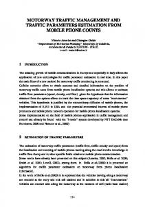
Figure 9: Aimsun2 screen shot: Zoom-in on a complex node in a highway network, simulated in Aimsun2. (Photo courtesy of TSS)
21