Home
Search
Collections
Journals
About
Contact us
My IOPscience
Advances in Computational High-Resolution Mechanical Spectroscopy HRMS Part I: Logarithmic Decrement
This article has been downloaded from IOPscience. Please scroll down to see the full text article. 2012 IOP Conf. Ser.: Mater. Sci. Eng. 31 012018 (http://iopscience.iop.org/1757-899X/31/1/012018) View the table of contents for this issue, or go to the journal homepage for more
Download details: IP Address: 213.134.187.143 The article was downloaded on 22/02/2012 at 11:58
Please note that terms and conditions apply.
6th EEIGM International Conference on Advanced Materials Research IOP Conf. Series: Materials Science and Engineering 31 (2012) 012018
IOP Publishing doi:10.1088/1757-899X/31/1/012018
Advances in Computational High-Resolution Mechanical Spectroscopy HRMS. Part I - Logarithmic Decrement M Majewski1, A Piłat2, L B Magalas1 1
AGH University of Science and Technology, Faculty of Metals Engineering and Industrial Computer Science, al. Mickiewicza 30, 30-059 Kraków, Poland 2 AGH University of Science and Technology, Faculty of Electrical Engineering, Automatics, Computer Science and Electronics, al. Mickiewicza 30, 30-059 Kraków, Poland
E-mail:
[email protected] Abstract. The comparison between different methods used to compute the logarithmic decrement in high-resolution mechanical spectroscopy (HRMS) is analyzed. The performance of parametric OMI method (Optimization in Multiple Intervals) and interpolated discrete Fourier transform (IpDFT) methods are investigated as a function of the sampling frequency used to digitize free decaying oscillations in lowfrequency resonant mechanical spectrometers. It is clearly demonstrated that a new Yoshida-Magalas (YM) method is the most powerful IpDFT-based method which outperforms the standard Yoshida (Y) method and other DFT-based methods. Four IpDFT methods and the OMI method are carefully analyzed as a function of the sampling frequency. The results presented in this work clearly show that the relative error in the estimation of the logarithmic decrement depends both on the length of free decaying signal and on the sampling frequency. The effect of the sampling frequency was not yet reported in the literature. The performance of different methods used in the computations of the logarithmic decrement can be listed in the following order: (1) the OMI, (2) the Yoshida-Magalas YM, (3) the Yoshida-Magalas YMC, and finally (4) the Yoshida Y.
1. Introduction High-resolution mechanical spectroscopy HRMS [1-3] requires new computing tools and algorithms to determine the logarithmic decrement δ and the resonant frequency f 0 from free decaying oscillations with high precision and very low dispersion in experimental points. In addition, it is also expected that computations of the δ and f 0 will be independent on small external perturbations (i.e. the ZPD effect [7, 9], defined as the deployment of the center of damped harmonic oscillations) while computing time must be reasonably short. These, frequently contradictory requirements, are difficult to be fulfilled [1-20]. These problems are tackled in this work. Computations of the logarithmic decrement δ will be analyzed here as a function of the length of free decaying oscillations for two different sampling frequencies: 1 kHz (usually used in low-frequency resonant mechanical spectrometers) and 6 kHz (it will be demonstrated here that f S = 6 kHz yields the best results for lowfrequency mechanical spectrometers operating around the resonant frequency f 0 ≈ 1 Hz). It should be emphasized that computation techniques used in HRMS depend on too many parameters, which is why the computational problem is a multi-dimensional task [1-13].
Published under licence by IOP Publishing Ltd
1
6th EEIGM International Conference on Advanced Materials Research IOP Conf. Series: Materials Science and Engineering 31 (2012) 012018
IOP Publishing doi:10.1088/1757-899X/31/1/012018
To elucidate this problem the effect of the length of the signal L and the sampling frequency f S on computed values of the logarithmic decrement are investigated. HRMS can provide better insight into a number of relaxation processes involving e.g. interaction of dislocations with mobile points defects (Dislocation-Enhanced Snoek Effect DESE and Snoek-Köster relaxation in bcc metals and alloys [14-20]), Bordoni relaxations, study of phase transitions and a number of transient phenomena frequently observed in mechanical loss measurements of different materials. It is noted that the OMI method (Optimization in Multiple Intervals) [1-8] and the YoshidaMagalas YM method can be successfully used to analyze free decaying oscillations biased by the ZPD effect [7, 9] which accompanies phase transitions and dislocation-induced phenomena.
2. Results and Discussion The exponentially damped time-invariant harmonic oscillations (free decaying oscillations, A(t ) ) embedded in an experimental noise εw(t) can be described using the digitized data Ai (t ) and ti acquired from free decaying signal [1, 2]:
A(t ) = A0e − δ f 0 t cos(2π f 0 t + ϕ ) + ε w (t ) + dc ,
(1)
where A0 is the maximal strain amplitude of a sample mounted in a mechanical spectrometer, t is a continuous time in seconds, −π < φ ≤ π is the phase of the signal A(t ) in radians, and dc is an offset. The noise εw(t) corresponds here to the signal-to-noise ratio S/N= 32 dB [1-7]. The logarithmic decrement δ can be computed from Eq. (2) [12]
−3 Im R −1 δ = 2π 3 Re s1 − R −1
(2)
while
R=
F ( s1 ) − 2 F ( s2 ) + F ( s3 ) , F ( s2 ) − 2 F ( s3 ) + F ( s4 )
(3)
where F ( s1 ), F ( s2 ), F ( s3 ), F ( s4 ) denote the magnitude of DFT bins [1-3, 12, 13, 21]. Three new interpolated discrete Fourier transform (IpDFT) methods: the Yoshida-Magalas methods (the YM, the YMC, and the YL [1-3]) and the original Yoshida method (Y) [12] use four DFT bins ( F ( s1 ), F ( s2 ), F ( s3 ), F ( s4 ) ) and a rectangular window [21]. The YL method differs from the Y method by the use of a fixed length of the signal A(t ) [1]. The YM method uses four optimal values of the DFT bins [1-3] whereas the YMC differs from the YM method by using a complete number of oscillations [1-3]. The Yoshida method [12] and other IpDFT methods were recently reviewed in [13]. The systematic errors induced by spectral leakage and a picket fence effect were also discussed in [13]. Detailed mathematical description of IpDFT methods used in this work (i.e. the YM, the YMC, and the YL) will be described elsewhere. 2
6th EEIGM International Conference on Advanced Materials Research IOP Conf. Series: Materials Science and Engineering 31 (2012) 012018
IOP Publishing doi:10.1088/1757-899X/31/1/012018
The performance of four IpDFT methods and the OMI method [1-8] for low damping level (δ = 5×10⁻⁴, f 0 = 1.12345 Hz) is analyzed here for two sampling frequencies: f S = 1 kHz and
f S = 6 kHz. It should be emphasized that the effect of the sampling frequency, f S , was not investigated in the literature [4, 8]. The results of computing the logarithmic decrement δ for a set of 100 free decays are reported here as a function of the length of free decaying signals L [1-3, 5, 7] (in seconds and/or as a function of the number of oscillations Losc) for two sampling frequencies, f S . Each free decaying signal A(t ) was embedded in statistically different experimental noise defined by the same S/N ratio. The results of computations obtained from the OMI and IpDFT methods are offset independent [3, 7]. Figures 1, 2, 5, and 6 demonstrate that the OMI method (the results are illustrated by the 1st set of computed δ values vertically plotted from the left side) outperforms IpDFT methods: the YM, the YMC, the YL , and the Y (the 2nd – 5th set of computed δ values vertically plotted) for all lengths of analyzed signals A(t ) . It should be emphasized that the Yoshida method generates the highest dispersion in δ values and the highest relative error γ δ (Figs. 2 and 6), the highest minimal γ δ
min
,
and the maximal γ δ max relative errors (Figs. 3, 7). The Y method returns the highest standard deviation too (Figs. 4, 8). It is convincingly demonstrated that the precision in computing the logarithmic decrement depends on the length of the signal while each method shows different performance. The Yoshida method returns strong dispersion for some well defined lengths of the signal A(t ) as a natural consequence of the relationship between the sampling and the resonant frequencies, and the fixed number of data points used in the algorithm [12] (e.g. Figs. 1, 5). That is why the sampling frequency f S is a key factor which affects the performance of the Yoshida method, Y. Computations of the δ for too short oscillations inevitably returns very strong dispersion (Figs. 1(a), 2(a) and 5(a), 6(a)). Is noteworthy that among four IpDFT methods the best performer is always the Yoshida-Magalas YM method [1-3]. Figures 1, 2 and 5, 6 indicate that the YMC method should be used to compute the δ from short free decaying signals. Figures 3 and 7 illustrate the performance of the IpDFT methods and the OMI method defined by the smallest relative error γ δ , the smallest minimal γ δ min and the maximal γ δ max relative error in the estimation of the δ, that is, the smallest dispersion of experimental points in mechanical loss measurements.
An increase in the sampling frequency, from 1 kHz to 4 kHz, reduces the dispersion by around 50 %. Further increase up to 6 kHz yields the best estimation for the δ for all lengths of the free decaying signals and generates the smallest computing errors (compare Figs. 1 - 4 and Figs. 5 - 8).
3. Conclusions The performance of different methods to compute the logarithmic decrement for low damping level (δ = 5×10⁻⁴ ) can be listed in the following order: (1) the OMI, (2) the Yoshida-Magalas YM, (3) the YMC, and the Yoshida (Y). The YM method outperforms other IpDFT methods [1-3, 12, 13] including the classic Yoshida method [12]. The YM method yields the smallest dispersion in experimental points of the logarithmic decrement δ for different lengths of free decaying oscillations and different sampling frequencies. The parametric OMI method is considered as the ‘gold standard’ in lowfrequency high-resolution mechanical spectroscopy HRMS [1, 2]. It is emphasized that the sampling frequency is an important factor to obtain the lowest dispersion of experimental points, that is, the
3
6th EEIGM International Conference on Advanced Materials Research IOP Conf. Series: Materials Science and Engineering 31 (2012) 012018
IOP Publishing doi:10.1088/1757-899X/31/1/012018
(a) -4
δ x10
4
20
8.90 t [s]
6.23
4.45 x 10
OMI YM YM
15
C
10
Y
5
Y
L
0 5
7
10
Losc
(b)
(c) -4
δ x 10
4
5.4
53.41 t [s]
44.50
35.60 x 10
5.2 5 4.8 40
45
50
55
60 L osc
(d)
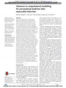
Figure 1. The effect of the sampling frequency f S = 1 kHz on dispersion of 100 values of the logarithmic decrement δ computed according to OMI, YM, YMC, YL, and Y methods as a function of the length of free decaying signals (i.e. the number of oscillations Losc .) (a) Losc = 5, 7, 10, (b) Losc = 15, 20, 25, 30, (c) Losc = 40, 50, 60, (d) Losc = 70, 80, 90, and 100. Computed values of the δ, displayed on vertical plots, correspond to a set of 100 different free decaying noisy oscillations (S/N = 32 dB) characterized by the same value of the δ = 0.0005 and the resonant frequency f0 = 1.12345 Hz.
4
6th EEIGM International Conference on Advanced Materials Research IOP Conf. Series: Materials Science and Engineering 31 (2012) 012018
IOP Publishing doi:10.1088/1757-899X/31/1/012018
(a) 4.45
γ [%]
400
6.23
8.90
t [s] OMI YM YM
200
C
Y
δ
L
Y
0 -200
5
7
10
Losc
(b)
(c) 35.60
53.41 t [s]
44.50
δ
γ [%]
5 0 -5 40
45
50
55
60 L
osc
(d)
Figure 2. The effect of the sampling frequency f S = 1 kHz on the relative errors γδ obtained for computations of the logarithmic decrement δ shown in Fig. 1 as a function of the length of free decaying signals (i.e. the number of oscillations Losc .) (a) Losc = 5, 7, 10, (b) Losc = 15, 20, 25, 30, (c) Losc = 40, 50, 60, (d) Losc = 70, 80, 90, and 100.
5
6th EEIGM International Conference on Advanced Materials Research IOP Conf. Series: Materials Science and Engineering 31 (2012) 012018
IOP Publishing doi:10.1088/1757-899X/31/1/012018
300
δ
max( γ ), min( γ ) [%]
(a) OMI YM YM C
200
Y
L
100
Y
δ
0
-100 5
7
15 L
10
osc
δ
max ( γ ), min ( γ ) [%]
(b) 5
δ
0
-5 20
30
40
50
60
70
80
Figure 3. The effect of the sampling frequency f S = 1 kHz on the minimal
γ δ min
100 L
90
osc
γδ
and the maximal
max
relative errors obtained for computations of the logarithmic decrement δ shown in Fig. 1. (a) Losc = 5, 7, 10, 15, (b) Losc = 20, 25, 30, 40, 50, 60, 70, 80, 90, and 100.
(a) -4
x 10 4
OMI YM YM
σ
3
C
Y
L
2
Y
1 5
7
15 L osc
10
(b) -6
x 10
σ
10
5
0 20
30
40
50
60
70
80
Figure 4. The effect of the sampling frequency f S = 1 kHz on the standard deviation
90
100 L
osc
σ obtained for computations
of the logarithmic decrement δ shown in Fig. 1. (a) Losc = 5, 7, 10, 15, (b) Losc = 20, 25, 30, 40, 50, 60, 70, 80, 90, and 100.
6
6th EEIGM International Conference on Advanced Materials Research IOP Conf. Series: Materials Science and Engineering 31 (2012) 012018
IOP Publishing doi:10.1088/1757-899X/31/1/012018
(a) 4.45
20
8.90 t [s]
6.23
OMI YM YM
4
15
δ x 10
C
Y
10
L
Y 5 0 5
7
10
Losc (b)
-4
δ x10
4
7
x13.35 10
17.80
22.25
20
25
26.70 t [s]
6 5 4 15
30 L
osc
(c) -4 35.60
53.41 t [s]
44.50
x 10
δ x10
4
5.4 5.2 5 4.8 4.6 40
45
50
60 L
55
osc
(d) -4
5.3
71.21
62.31 x 10
89.01 t [s]
80.11
δ x10
4
5.2 5.1 5 4.9 4.8 70
75
80
85
90
95
100 L
osc
Figure 5. The effect of the sampling frequency f S = 6 kHz on dispersion of 100 values of the logarithmic decrement δ computed according to OMI, YM, YMC, YL, and Y methods as a function of the length of free decaying signals (i.e. the number of oscillations Losc .) (a) Losc = 5, 7, 10, (b) Losc = 15, 20, 25, 30, (c) Losc = 40, 50, 60, (d) Losc = 70, 80, 90, and 100. Computed values of the δ, displayed on vertical plots, correspond to a set of 100 different free decaying noisy oscillations (S/N = 32 dB) characterized by the same value of the δ = 0.0005 and the resonant frequency f0 = 1.12345 Hz.
7
6th EEIGM International Conference on Advanced Materials Research IOP Conf. Series: Materials Science and Engineering 31 (2012) 012018
IOP Publishing doi:10.1088/1757-899X/31/1/012018
(a) 4.45
400
6.23
8.90
t [s] OMI YM YM
γ [%]
200
C
Y
δ
L
Y
0 -200
5
7
10
Losc
(b) 40
13.35
17.80
22.25
20
25
26.70 t [s]
δ
γ [%]
20 0 -20 15
30
Losc
(c) 35.60
53.41 t [s]
44.50
δ
γ [%]
5 0 -5 40
45
50
60 L
55
osc
(d) 89.01 t [s]
80.11
71.21
62.31
δ
γ [%]
5
0
-5 70
75
80
85
90
95
100 L
osc
Figure 6. The effect of the sampling frequency f S = 6 kHz on the relative errors γδ obtained for computations of the logarithmic decrement δ shown in Fig. 5 as a function of the length of free decaying signals (i.e. the number of oscillations Losc .) (a) Losc = 5, 7, 10, (b) Losc = 15, 20, 25, 30, (c) Losc = 40, 50, 60, (d) Losc = 70, 80, 90, and 100.
8
6th EEIGM International Conference on Advanced Materials Research IOP Conf. Series: Materials Science and Engineering 31 (2012) 012018
IOP Publishing doi:10.1088/1757-899X/31/1/012018
300
δ
max( γ ), min( γ ) [%]
(a) OMI YM YMC
200
YL
δ
100
Y
0
-100
5
7
15 L
10
osc
δ
max ( γ ) , min ( γ ) [%]
(b) 10 5
δ
0 -5 20
30
40
50
60
70
80
Figure 7. The effect of the sampling frequency f S = 6 kHz on the minimal
γ δ min
100 L
90
osc
and the maximal
γδ
max
relative errors obtained for computations of the logarithmic decrement δ shown in Fig. 5. (a) Losc = 5, 7, 10, 15, (b) Losc = 20, 25, 30, 40, 50, 60, 70, 80, 90, and 100.
(a) -4
4
x 10
OMI YM YM
σ
3
C
Y
L
2
Y
1 0
5
7
15 L osc
10
(b) -6
x 10
σ
15 10 5 0 20
30
40
50
60
70
80
Figure 8. The effect of the sampling frequency f S = 6 kHz on the standard deviation of the logarithmic decrement δ shown in Fig. 5. (a) Losc = 5, 7, 10, 15, (b) Losc = 20, 25, 30, 40, 50, 60, 70, 80, 90, and 100.
9
90
100 L osc
σ obtained for computations
6th EEIGM International Conference on Advanced Materials Research IOP Conf. Series: Materials Science and Engineering 31 (2012) 012018
IOP Publishing doi:10.1088/1757-899X/31/1/012018
lowest level of computing errors. It is concluded that the sampling frequency f S = 6 kHz provides much better results as compared to usually used
f S = 1 kHz in low-frequency mechanical
spectrometers operating around the resonant frequency f 0 ≈ 1 Hz. The OMI method and the Yoshida-Magalas YM method are recommended to compute the logarithmic decrement δ from exponentially damped time-invariant harmonic oscillations embedded in an experimental noise recorded in low-frequency mechanical spectrometers ( f 0 ≈ 1 Hz.) This conclusion is valid for low damping level (δ = 5×10⁻⁴.) Acknowledgements. This work was supported by Polish National Science Centre under grant No N N507 249040 and No N N507 446639.
References
[1] [2] [3] [4] [5] [6] [7] [8] [9] [10] [11] [12] [13] [14] [15] [16] [17] [18] [19] [20] [21]
Magalas L B and Majewski M 2011 Sol. St. Phen. 184 467-472 Magalas L B and Majewski M 2011 Sol. St. Phen. 184 473-478 Majewski M 2011 PhD Thesis, AGH University of Science and Technology, Kraków, Poland Magalas L B 2006 Sol. St. Phen. 115 7-14 Magalas L B and Majewski M 2008 Sol. St. Phen. 137 15-20 Magalas L B and Malinowski T 2003 Sol. St. Phen. 89 247-260 Magalas L B and Majewski M 2009 Mater. Sci. Eng. A 521-522 384-388 Magalas L B and Stanisławczyk A 2006 Key Eng. Materials 319 231-240 Magalas L B and Piłat A 2006 Sol. St. Phen. 115 285-292 Magalas L B 2003 Sol. St. Phen. 89 1-22 Etienne S, Elkoun S, David L and Magalas L B 2003 Sol. St. Phen. 89 31-66 Yoshida I, Sugai T, Tani S, Motegi M, Minamida K and Hayakawa H 1981 J. Phys. E: Sci. Instrum. 14 1201-1206 Duda K, Magalas L B, Majewski M and Zieliński T P 2011 IEEE Transactions on Instrumentation and Measurement 60 3608-3618 Magalas L B, Dufresne J F and Moser P 1981 J. de Phys. 42 (C-5) 127-132 Magalas L B, Moser P and Ritchie I G 1983 J. de Phys. 44 (C-9) 645-649 Magalas L B and Gorczyca S 1985 J. de Phys. 46 (C-10) 253-256 Rubianes J, Magalas L B and Fantozzi G 1987 J. de Phys. 48 (C-8) 185-190 Ngai K L, Wang Y N and Magalas L B 1994, J. Alloy Compd. 211/212 327-332 Magalas L B 1996 J. de Phys. IV 6 (C8) 163-172 Magalas L B 2003 Acta Metallurgica Sinica 39 1145-1152 Brigham E O 1988 The Fast Fourier Transform FFT and its Applications, Prentice Hall Signal Processing Series
10