17th International Conference on the Application of Computer Science and Mathematics in Architecture and Civil Engineering K. G¨urlebeck and C. K¨onke (eds.) Weimar, Germany, 12–14 July 2006
ADVANCES IN FLUID-STRUCTURE INTERACTION Wolfgang A. Wall∗ , Christiane F¨orster, Malte Neumann and Ekkehard Ramm ∗
Chair of Computational Mechanics, Technical University of Munich Bolzmannstraße 15, 85747 Garching, Germany E-mail:
[email protected]
Keywords: fluid-structure interaction, strong coupling schemes, stability Abstract. For the dynamic behavior of lightweight structures like thin shells and membranes exposed to fluid flow the interaction between the two fields is often essential. Computational fluid-structure interaction provides a tool to predict this interaction and complement or eventually replace expensive experiments. Partitioned analyses techniques enjoy great popularity for the numerical simulation of these interactions. This is due to their computational superiority over simultaneous, i.e. fully coupled monolithic approaches, as they allow the independent use of suitable discretization methods and modular analysis software. We use, for the fluid, GLS stabilized finite elements on a moving domain based on the incompressible instationary Navier-Stokes equations, where the formulation guarantees geometric conservation on the deforming domain. The structure is discretized by nonlinear, three-dimensional shell elements. Commonly used sequential staggered coupling schemes may exhibit instabilities due to the so-called artificial added mass effect. As best remedy to this problem subiterations should be invoked to guarantee kinematic and dynamic continuity across the fluid-structure interface. Since iterative coupling algorithms are computationally very costly, their convergence rate is very decisive for their usability. To ensure and accelerate the convergence of this iteration the updates of the interface position are relaxed. The time dependent, ’optimal’ relaxation parameter is determined automatically without any user-input via exploiting a gradient method or applying an Aitken iteration scheme.
1
1
INTRODUCTION
Robust and reliable numerical simulation of complex fluid-structure interaction problems remains challenging. In particular shell structures exhibit highly nonlinear and sensitive physical behavior which clearly also transfers to the numerical schemes [18]. Within this work a partitioned fluid-structure interaction algorithm is considered. Partitioned algorithms allow for specificly designed numerical approaches on the single fields and yield a modular software structure. Finite elements are employed for the spatial discretization of both fields, i.e. the fluid and structural part. The arbitrary Lagrangian Eulerian (ALE) formulation is used on the fluid field allowing to track the interface exactly which is crucial for accurate interaction. The ALE approach demands for the solution of the fluid equations on a moving domain. Correct determination of coupling information at the interface including geometric conservation on the entire fluid domain is essential to obtain a robust overall algorithm which is both stable and accurate [8, 7]. While being attractive in terms of efficiency staggered coupling schemes employed for the interaction of incompressible flows and slender, lightweight structures may exhibit an inherent instability. This so-called artificial added mass effect is not an artifact of a particular discretization scheme but rather a built-in property of the coupling scheme itself. Consequently the instability does not decrease when the accuracy of the temporal discretization is increased. An analysis reveals that the instability stems from too high eigenvalues of the amplification operator inherent in the coupling scheme. Thus for a robust fluid-structure interaction algorithm the prize has to be payed and the scheme has to be formulated iteratively. Iterative fluid-structure interaction schemes for three-dimensional problems demand immense computational resources and easily touch the limit of todays computer power. Thus efficiency is a major concern in terms of an efficient coupling algorithm as well as efficient solvers in particular on the fluid domain which consumes by far the largest part of the overall computing time [17]. The instability of the staggered or weakly coupled scheme transfers to parameter sensitivity in the iteratively staggered scheme. Parameter combinations which cannot be treated by a weakly staggered scheme demand for a high number of iterations in the iteratively staggered case and also induce an upper bound on the relaxation parameter ω to enable convergence [4]. Two methods to automatically determine the proper amount of relaxation required are given. Numerical examples demonstrate the method. 2 2.1
GOVERNING EQUATIONS AND DISCRETIZATION Structure field
The problems of interest frequently include large structural deformations which have to be considered within the structural formulation. The structure is thus described by the equations of geometrically nonlinear elastodynamics on the structural domain ΩS ¨ ~ + ρS~b, ρS d~ = ∇ · S
(1)
with appropriate initial and boundary conditions. Here d~ represents the vector field of structural displacements, ρS the structural density and ~b the structural body forces. The over-set dot ¨ ~ denotes the second Piolarepresents time derivatives, i.e. d~ is the structural acceleration field. S 2
physical space χ2
ϕ(χ, t) χ2 χ1
reference space
x2
χ1
Ωt
x1
Figure 1: Sketch of ALE mapping
~ through a St. VenantKirchhoff stress tensor related to the Green-Lagrange strain tensor E Kirchhoff constitutive relation. ³ ´ ~=C ~ :E ~ ~ = 1 F~ T · F~ − I~ , S with E (2) 2 where F~ represents the deformation gradient tensor. A variety of different finite elements is employed for spatial discretization. Particularly shell elements are used that offer reliable results even for large deformations [1, 2, 11]. After discretization in space the semidiscrete structural equation reads ¨ + DS d˙ + NS (d) = f S MS d (3) where damping has been included. In the matrix equation (3) the symbols MS and DS represent the structural mass and damping matrices while NS and f S denote the internal and external ¨ represents forces, respectively. The nodal displacement vector is given by d while d˙ and d discrete nodal velocities and accelerations. In the present approach this system is solved using the ’generalized-α method’ of Chung and Hulbert [5] along with consistent linearization and a Newton-Raphson iterative scheme. The ’generalized-α method’ is an implicit, one-step time integration scheme based on Newmark like approximations in the time domain. It exhibits controllable numerical dissipation and allows for unconditional stable solutions of nonlinear dynamics. 2.2
Fluid field
A Newtonian fluid is considered governed by the incompressible Navier-Stokes equations. The flow equations determining the unknown fields of the velocity ~u and the kinematic pressure p read ¯ ∂u ¯¯ + ∇ (u ⊗ u) − 2ν∇ · ε(u) + ∇p = f F in ΩF × (0, T ), (4) ∂t ¯x ∇ · ~u = 0 in ΩF × (0, T ). (5) The parameter ν = µ/ρF denotes the kinematic viscosity where µ represents the viscosity and ρF density of the fluid. The vector field f~F denotes the specific body force on the fluid. In order to formulate the balance of momentum in a deforming ALE frame of reference the coordinate system χ which follows the motion of the respective boundaries while deforming arbitrary in between is introduced as sketched in figure 1. The geometrical location of a mesh 3
point is obtained from the unique mapping x = ϕ(χ, t). Employing the reference system χ and Reynolds transport theorem equation (4) can be reformulated on moving grids as ¯ © ¡ ¢ ª ∂(uJt ) ¯¯ + ∇ · u ⊗ (u − uG ) − 2ν∇ · ε(u) + ∇p Jt = f F Jt , (6) ¯ ∂t χ where Jt = det(∂x/∂χ) denotes the time dependent Jacobian of the mapping and uG = ∂x/∂t|χ represents the velocity of the reference system, i.e. in the discretized case the grid velocity. It is very common to use the finite volume method for the discretization of flow problems. In this case equation (6) has to be used as point of departure for a discretization in space which results in a difficulty with the temporal discretization of the mass term. This difficulty can be seen in the weighted residual formulation where the mass term yields a time derivative of an integral over a temporally changing domain. The time discretization of this term is rather cumbersome. Thus extra effort has to be made in order to satisfy the geometric conservation law resulting in the need for temporal averaging of either geometries or fluxes within a time step when a finite volume discretization is applied [7]. Depending on the temporal discretization scheme different versions of the geometric conservation law, i.e. different discrete geometric conservation laws (DGCL) and thus averaging schemes, have to be used [12] if (6) is discretized directly. Discretization by means of finite elements allows to circumvent these difficulties. The geometric conservation law itself is given in the strong form by ∂Jt = J t ∇ · uG ∂t
(7)
linking the temporal change of the domain to the domain velocity. Equation (7) can be incorporated into (6) yielding a local form of the balance of momentum which can straightforwardly be discretized in time and space ¯ ¡ ¢ ∂~u ¯¯ + ~u − ~uG · ∇~u − ∇ · σ = f~F in ΩF × (0, T ), (8) ¯ ∂t χ where the stress tensor of a Newtonian fluid is given by σ = −pI + 2νε(~u) and
ε(~u) =
¢ 1¡ ∇~u + ∇~uT 2
denotes the strain rate tensor. The local ALE form (8) avoids the difficulties inherent in (6) and allows to preserve the stability as well as the order of accuracy which a time discretization scheme exhibits on fixed grids. As the geometric conservation law (7) has been incorporated prior to discretization the need for different DGCL schemes is removed [8]. The partial differential equation (8) is subject to appropriate initial and boundary conditions. After discretization in space equation (8) yields the matrix representation MF u˙ + NF (u)u + KF u + Gp = f F GT u = 0,
(9)
where MF represents the fluid mass matrix, NF (u) and KF denote the nonlinear convective and viscous matrix, respectively, and f F is the nodal vector of the integrated body and boundary 4
forces. The matrix G represents the discrete gradient operator. All fluid matrices depend on the unknown velocity u due to additional nonlinearities introduced by stabilization terms [19]. To evaluate the above matrices the integration of the weak form of all terms is performed over the actual configuration at time level n + 1 ensuring geometric conservation [8] as described above. Second order accurate backward differencing (BDF2) scheme or the one-step-θ time integration both fully implicit are used to discretize (9) in time. The occurring nonlinearities are dealt with using a Newton iteration scheme. 3
PARTITIONED DIRICHLET-NEUMANN ALGORITHM
The overall analysis is based on an element-wise, i.e. non-overlapping partitioned approach. This allows single field solvers, tailored to meet the needs of structural and fluid fields. The wet structural surface is thus the ’natural’ coupling interface Γ. 3.1
Coupling boundary conditions
A key requirement for the coupling schemes is to fulfill two coupling conditions: the kinematic and the dynamic continuity across the interface at all times. Kinematic continuity requires that the position of structure and fluid boundary are equal at the interface, while dynamic continuity means that all tractions at the interface are in equilibrium. In a continuous setting the boundary conditions at the coupling interface Γ read ¯ ∂rΓ (t) ¯¯ G dΓ (t) · n = rΓ (t) · n and uΓ (t) · n = uΓ (t) · n = (10) ·n ∂t ¯χ σ SΓ (t) · n = σ FΓ (t) · n
(11)
with n and r denoting the unit normal vector on the interface and the position of the reference system, respectively. Here σ SΓ represents the Cauchy stress tensor of the structural field. Satisfying the kinematic continuity leads to mass conservation at Γ, satisfying the dynamic continuity yields conservation of linear momentum, and energy conservation requires to simultaneously satisfy both continuity equations. Due to different time discretization schemes on the three fields of structure, fluid and mesh exact satisfaction of all boundary conditions at all times will not be possible in a discrete setting. Rather discrete versions of the coupling conditions (10) and (11) can be found. Assuming for brevity a sticking mesh which follows the deformation of the wet surface Γ in normal and tangential directions the discrete displacement continuity reads = dn+1 rn+1 Γ , Γ i.e. at the end of a new time step the mesh and structural interface displacements are equal. The new fluid velocity at the interface also depends upon the mesh (and thus the structural) displacement. For the time discretization schemes considered here namely BDF2 and one-stepθ, the fluid velocity at the wet interface is given by rn+1 − rnΓ Γ − unΓ , (12) ∆t which ensures that the discrete velocity function integrated in time yields the actual interface position and thus geometric conservation and consequently a correct mass balance is satisfied at the boundary. un+1 =2 Γ
5
The temporal interpolation of the mesh velocity is crucial to preserve the formal order of accuracy. In order to guarantee the second order accuracy of the overall algorithm a second order interpolation of the mesh velocity is required. For either time discretization of the fluid velocities u BDF2 is used to interpolate the mesh velocity uG Γ yielding uG,n+1 = Γ
3 rn+1 − 4 rnΓ + rΓn−1 Γ . 2 ∆t
(13)
The difference of un+1 and uG,n+1 is regarded a discretization error. Γ Γ The discrete dynamic boundary condition yields f ΓS,n+1 = ρF f F,n+1 , Γ where the fluid forces have to be multiplied by the fluid density in order to account for the normalization of the Navier-Stokes equation (8) by the density. To obtain accurate coupling forces consistent with the spatial discretization by finite elements nodal forces have to be evaluated. Assuming that no body forces are present and using BDF2 time discretization the consistent nodal forces read ¡ F ¡ n ¢ ¢ n+1 3 1 F n+1 F F n−1 n+1 f F,n+1 = M M u + N 4 u − u (14) + K u + G p − Γ Γ Γ Γ 2 ∆t Γ 2 ∆t Γ where the subscript Γ denotes the lines of the original matrices belonging to the interface degrees of freedom. Consistent nodal forces share the formal order of accuracy of the primary variable and naturally contain the contribution of viscous forces. In contrast to forces obtained from the discrete stresses, nodal forces obtained from (14) ensure conservation [13]. They further fit into a nodal based data structure and are thus easy and efficiently to implement. Consistent nodal fluid forces are a key ingredient for accurate coupling on moderately fine meshes. 3.2
Partitioned schemes
The partitioned analysis schemes under consideration with synchronous time discretizations in the fluid and structural part can be cast in a unified algorithmic framework. They are discussed in detail in Mok [21, 16]. In the following, (·)I and (·)Γ denotes variables or coefficients in the interior of a subdomain Ωj and on the coupling interface, respectively, while a vector without any of the subscripts I and Γ comprises degrees of freedom on the entire subdomain including interior and interface. In addition to the structural domain ΩS and the fluid domain ΩF a mesh domain ΩM is introduced here which coincides with the fluid domain or parts of it. The mesh automatically determines the position of the internal fluid nodes by solving the pseudo structural equation KM r = f M , where KM represents the mesh stiffness matrix, r denotes the nodal position vector and the right hand side vector f M stems from Dirichlet boundary conditions on the mesh domain. In every time interval [tn , tn+1 ] the following algorithmic steps have to be performed in order to compute the new coupled solution at tn+1 , starting from a known state of motion at tn . n+1 1. Compute structural predictor dn+1 (see subsection Γ,0 for the interface displacements at t 3.3). Set i = 0
2a. Solve fluid mesh ΩM for new positions. M n+1 n+1 KM II rI,i+1 = −KIΓ rI,i+1
with Dirichlet b.c. 6
n+1 rn+1 I,i+1 = dΓ,i
2b. Derive new grid velocity at time level n+1 in compliance with the geometric conservation law and the required accuracy1 . For second order accuracy equation (13) can be used. 2c. Derive new fluid velocity along wet surface Γ which is used as Dirichlet boundary condition according to equation (12). 2d. Solve fluid partition ΩF on new mesh configuration (at n + 1) for new fluid velocity and pressure fields, i.e. solve a temporally discretized version of (9). 3. Determine consistent nodal fluid forces by inserting the obtained fluid solution and Dirichlet boundary conditions into the equations belonging to the wet surface Γ as done in equation (14). 4. Solve structure partition ΩS , i.e. a temporally discretized version of equation (3), with n n+1 oT ˜ . Neumann b.c. f S,n+1 for new structural displacements dn+1 := d dn+1 i+1
Γ,i+1
Γ,i+1
I,i+1
5a. For iterative schemes only: Determine suitable relaxation parameter ωi ∈ R+ (see subsection 3.4). 5b Compute relaxed update of predicted interface position. n+1 ˜ n+1 dn+1 Γ,i+1 = ωi dΓ,i+1 + (1 − ωi )dΓ,i
(15)
5c. Check convergence of interface displacements and/or residual. If not converged, then set i → i + 1 and go back to step 2. 6. Proceed to next time step by setting n → n + 1. 3.3
Weak coupling approaches and artificial added mass effect
A particularly appealing way to solve the coupled problem is a sequentially staggered formulation which demands for only one solution of either field per time step. While the fluid and structural domain are solved implicitly the coupling information is exchanged once per time step which introduces an explicit feature. While being very promising in the sense of efficiency sequentially staggered algorithms may exhibit an inherent instability which increases with decreasing time step. Properties of the instability The problem has been described by Mok [21, 16] and its mathematical background has recently been provided by Causin et al. [4]. • With decreasing ∆t the instability occurs earlier. • The mass ratio between fluid and structure has a significant influence on the stability of F the staggered system. The bigger the mass ratio ρρS the worse the instability. • Numerical observations indicate that increased fluid viscosity increases the instability while increased structural stiffness offers a slightly decreasing effect. 1
The accuracy of the temporal interpolation of the mesh motion determines the overall temporal accuracy. Higher order overall accuracy can be sacrificed by using an interpolation of the mesh motion which is just first order [8].
7
• The actual onset of unconditional instability depends upon the particular combination of temporal discretization items. Especially the first point indicates that the instability is not due to a lack of temporal accuracy introduced by the explicit character of the coupling scheme. Artificial added mass effect As the not fully balanced fluid forces have the effect of an extra mass on the structural interface degrees of freedom the destabilization has been termed artificial added mass effect [19]. An analysis shows that the instability is caused by too large eigenvalues of the amplification operator of the explicit step [4, 9]. Summarizing the steps 2. and 3. within the algorithm given in subsection 3.2 allows to identify the dimensionless added mass operator MA . This operator directly transfers the predicted nodal accelerations u˙ Γ at the interface Γ into the fluid forces f Γ exerted on the structure by f Γ = mF MA u˙ Γ , where mF denotes a characteristic fluid mass. The added mass operator MA contains the solution of the fluid problem in terms of forces along Γ caused by interface accerlation u˙ Γ [9]. Introducing this into the discrete linear and undamped structural equations and neglecting structural forces for the purpose of a stability analysis yields · S ¸· ¸ · S ¸· ¸ · ¸ ¨I MII MSIΓ d KII KSIΓ dI 0 (16) ¨ Γ + KSΓI KSΓΓ dΓ = −mF MA u˙ Γ . MSΓI MSΓΓ d Here the structural system of equations has been split into internal (subscript I) and interface (subscript Γ) degrees of freedom. Inserting the particular representation of the predictor and Dirichlet boundary condition allows to analyze the eigenvalue of the operator that transfers the interface displacements dΓ from time level n to n + 1. Here two different cases can be distinguished where dn+1 is either a function of a limited number of old interface positions Γ n n−1 n−2 (for example dn+1 = f (d Γ , dΓ , dΓ )) or it depends upon all previously calculated interface Γ 0 positions dn+1 = f (dnΓ , dn−1 Γ Γ , . . . , dΓ ). As shown in [9] this depends on the time discretization of the two fields as well as on the specific predictor and the way to obtain the Dirichlet boundary condition on the fluid field at Γ. In the first case an ‘instability condition’ of the form mF max µi > C1 mS
(17)
can be obtained, where mS represents a characteristic structural mass and µi denotes the ith eigenvalue of the added mass operator MA . The partitioned scheme is unstable if the condition (17) is satisfied. The limit C1 depends upon the particular details of the temporal discretization and decreases with increasing accuracy [9]. Thus the more accurate the scheme is the earlier it gets unstable with respect to the density ratio of fluid and structure. This effect can be observed when C1 is investigated for a number of different structural predictors used in step 1. of the algorithm given in subsection 3.2. A simple predictor which is zeroth order in time is given by n dn+1 Γ,P = dΓ . A first order predictor is
n ˙n dn+1 Γ,P = dΓ + ∆t dΓ
8
while
µ dn+1 Γ,P
=
dnΓ
+ ∆t
3 ˙ n 1 ˙ n−1 d − d 2 Γ 2 Γ
is a second order accurate predicted interface displacement. The instability limits obtained in [9] for the different structural predictors and backward Euler (BE) or second order backward differencing (BDF2) time discretization of the fluid equations are given in table 1. Similar results can be obtained when the temporal accuracy of other items of the overall algorithm (for example the interpolation order of the Dirichlet boundary condition required in step 2c.) of subsection 3.2 is increased. Table 1: Instability limit C1 for sequentially staggered fluid-structure interaction schemes depending upon the structural predictor and fluid time discretization scheme.
predictor
BE
BDF2
0th order 1st order 2nd order
3
3 2 3 10 1 6
3 5 1 3
In the second case where the interface displacements depend on all previously calculated 0 interface positions dn+1 = f (dnΓ , dn−1 Γ Γ , . . . , dΓ ) the problem gets even worse. Here an instability condition of the form C2 mF max µ > i mS n is obtained where n is the number of the time step. Thus the instability limit C2 /n decreases during the simulation and regardless of the density ratio a step will be reached at which the problem becomes unstable. When stabilized fluid elements are considered the analysis gets more complicated and the simple instability limits given in table 1 are not directly applicable any more. It can however be proven that for every sequentially staggered scheme a density ratio ρF /ρS exists at which the scheme becomes unstable [9]. Numerical investigations show that the instability limits are very restrictive when incompressible fluids are considered and stabilized finite elements are employed, effectively preventing stable computations by means of staggered algorithms. 3.4
Iterative staggered schemes
The only way to obtain a stable and accurate solution without changing the underlying physics are subiterations. These so-called iterative staggered schemes must then of course be designed to be as cheap and robust as possible. The iterative scheme described in the above algorithmic framework for fluid-structure interaction is due to Le Tallec et al. [15]. It can be interpreted as an iterative Dirichlet-Neumann substructuring scheme based on a preconditioned nonstationary Richardson iteration. This becomes obvious from the iterative evolution equation, ³ ´ mod,n+1 n+1 −1 n+1 dn+1 = d + ω S f − (S + S ) d i S F S Γ,i+1 Γ,i Γ,i Γ ext
9
which is reduced to the degrees of freedom on the interface Γ. SF and SS denote the Schur complement matrices of the fluid and structural fields, respectively, and f mod,n+1 is the external Γ ext load vector resulting after static condensation of the degrees of freedom in the interior of both subdomains. In this iterative scheme convergence is accelerated and ensured by the relaxed updates of the interface position. The iteration then converges to the simultaneous solution, exactly fulfilling the discrete coupling conditions. However a key question remains: How to choose optimal relaxation parameters ωi ? This is a rather sensitive question as relaxation is not always helpful in order to accelerate convergence. The instability observed at the sequentially staggered scheme transfers to the iteratively staggered algorithm demanding a relaxation parameter ωi < 1 to enable convergence [4]. The commonly used strategy to employ an experimentally (by trial end error) determined fixed parameter is unsatisfactory, because such a parameter is very problem-dependent, in general suboptimal especially for nonlinear problems, and it requires a careful, time consuming and difficult determination. Here two techniques are proposed which are both robust in the sense that they have problem-independent acceleration properties even for nonlinear systems, and user-friendly in the sense that relaxation parameters are determined automatically without any user-input being necessary. 3.4.1
Iterative substructuring scheme accelerated via gradient method
The first technique is an acceleration via the application of the gradient method (method of steepest descent) to the iterative substructuring scheme. This method also guarantees convergence. In every iteration a relaxation parameter ωi is computed by ωi =
gTi gi gTi gi ³ ´ = ¡ ¢ −1 S −1 F T gTi SS SF + SS gi gi S S gi + gi
(18)
which is locally optimal with respect to the actual search direction, i.e. the residual ³ ¡ F ¢ n+1 ´ −1 S ˜ n+1 − dn+1 . g i = SS f mod,n+1 − S + S dΓ,i = d Γ,i+1 Γ,i Γ ext A procedure for evaluating equation (18) without explicitly computing and storing the Schur complements SF and SS has been proposed in Wall et al. [20]. 3.4.2
Iterative substructuring scheme accelerated via the Aitken method
A second technique for explicitly calculating a suitable relaxation parameter is the application of Aitken’s acceleration scheme for vector sequences according to Irons et al. [14]. To obtain ωi the interfacial displacement difference is computed n+1 ˜ n+1 ∆dn+1 Γ,i+1 := dΓ,i − dΓ,i+1 .
The Aitken factor is obtained from µn+1 i
=
µn+1 i−1
+
¡
µn+1 i−1
¡ ¢ n+1 T ¢ ∆dn+1 ∆dn+1 Γ,i − ∆dΓ,i+1 Γ,i+1 −1 ¡ n+1 ¢ n+1 2 ∆dΓ,i − ∆dΓ,i+1
10
and yields the relaxation parameter . ωi = 1 − µn+1 i Even though a rigorous analysis of its convergence properties does not exist, numerical studies have shown that the Aitken acceleration for vector sequences applied to the fluid-structure interaction problems considered here shows a performance which is at least as good as the acceleration via the gradient method. Furthermore the evaluation of the relaxation parameters via the Aitken method is extremely cheap in terms of both CPU and memory and simple to implement. 4 4.1
EXAMPLES Vibrating U-pipe
Coriolis flowmeters are an elegant way to measure the mass flow rate in a pipe. The measuring unit inside such a flowmeter is a flexible tube which classically is U-shaped, clamped at both ends and passed by the flow. The pipe is subject to a forced vibration at angular frequency ωf which induces opposite and time dependent Coriolis forces within the fluid in the inflow and outflow part of the tube. Thus the resulting vibration is not just the enforced bending but accompanied by an amount of torsion depending upon the frequency ratio ft /ff where ft denotes the eigenfrequency of the torsional mode. Geometry and material parameters of the sample tube are given in figure 2 where the tube is fully clamped at the in- and outflow boundaries. In contrast to technical flowmeters the pipe geometry
0110 1010 0110 1001 10 10 10 10 inflow
outflow
y
A z 1.5 cm
2.0 cm
B
0.5 cm
1.5 cm
10.0 cm
diameter 1.0 cm
shell thickness: t = 0.1 cm
material structure: E = 1.0 × 10⁸ s2 gcm Poisson’s ratio: 0.4 g ρS = 1.5 cm 3 fluid: g ρF = 0.998 cm 3
x
2
ν = 0.01012 cm s
1.5 cm
Figure 2: Geometry and material of flowmeter tube
tube material is a rubber like compressible neo-Hookean type of material which yields large deflections of the overall system and thus allows to highlight the physical effect. Gravity points 11
in negative z-direction while the gravitational forces of the shell are neglected. The inflow velocity of the water inside the tube is prescribed to uy = 15 cm/s. The mesh of the tube itself consists of 5120 quad4 shell elements [1] enriched by means of the enhanced assumed strain method (EAS) to remove membrane shear locking inherent in linear elements. Further the Assumed Natural Strains method (ANS) is employed to avoid parasitic transverse shear strains, i.e. removing shear locking. Scaled director conditioning with C = 10.0 is employed to improve the conditioning of the resulting structural system of equations [10, 11]. The fluid domain is meshed by 11520 trilinear hex8 elements with residual based stabilization [19]. A major part of the fluid domain is accompanied by a mesh field consisting of 10240 pseudo structural hex8 elements. Thus the overall mesh while still being quite coarse for the problem consists of 26880 elements yielding a total of 94924 degrees of freedom on three fields. To adequately resolve the higher frequencies of interest a small time step of ∆t = 0.005 s is used. A harmonic force with a frequency of ff = 7.685 Hz which is close to the eigenfrequency of the torsional mode ft is applied on the tip of the clamped tube pointing in z-direction. The force is distributed over the area of the part of the pipe which is parallel to the x-axis. The induced oscillation is not just the expected bending but also an increasing torsional replay which is due to the Coriolis forces induced in the two arms of the pipe during the up and down cycles. In figure 3 the evolution of the vertical displacements at the points A and B is depicted along with the displacement difference. 0.6
vertical displacement in cm
0.4 0.2 0 -0.2 -0.4 -0.6 -0.8 -1 -1.2 -1.4 -1.6
5
5.5
9 7 7.5 8 8.5 time in s vertical displacement of point A vertical displacement of point B difference of vertical displacement of point A and point B 6
6.5
Figure 3: Vertical displacements at the two points A and B along with displacement difference between the respective points
In order to ensure the well-posedness of the problem the flow passing the tube as well as the gravitational forces have to be built up over a period in time. This startup was finished at 4.0 s when the system oscillated in the first bending mode and its corresponding eigenfrequency as 12
it can be seen in the first part of the diagram in figure 3. At 5.5 s the periodic vertical tip force is switched on creating a forced vibration on the first, the bending eigenmode of the structure. The evolution of the increasing contribution of the torsional mode can be detected from the increasing displacement difference of the two reference points A and B of the shell. In every cycle a portion of the bending energy is transfered to the torsional mode resulting in an increasing torsional oscillation. In figure 4 the deformed tube at different time instants is depicted. The figures show the x-z plane of the problem. The non-symmetric part of the structural response is entirely due to the interaction with the flowing water inside the tube. If the water is resting inside the tube no torsional displacement results. t = 9.87 s
t = 10.07 s
t = 9.945 s
t = 10.13 s
t = 10.005 s
t = 10.20 s
Figure 4: Deformation of the tube at different time instants
4.2
Flow in a collapsible tube
This example is concerned with the problem of viscous flow in an elastic tube. Elastic tubes collapse (buckle non-axisymmetrically) when the transmural pressure (internal minus external pressure) falls below a critical value. The tube’s large deformation during the buckling leads to a strong interaction between the fluid and the solid mechanics. To illustrate the tube’s behavior we consider its deformation in a procedure in which the flow rate is prescribed by means of a volumetric pump attached to the tube’s upstream end (see figure 5). We keep the fluid pressure at the tubes far downstream end constant, pdown = 0.0 and induce the tube’s collapse by increasing the chamber pressure. As the chamber pressure is increased, the transmural pressure decreases and first becomes negative (compressive) at the tube’s downstream end. When the compressive load exceeds a critical value, the axisymmetric deformation looses its stability and the tube buckles non-axisymmetrically. Figure 6 shows the tube’s wall deformation as the non-axisymmetric collapse increases.
13
g replacements 0.001 0.1 ib 0.2 1.0 pdown pup
pc ob
pe
u
pu
pd m1
pext u ˆ3 pressure chamber inflow boundary outflow boundary
m3
pe
m4
m3
Figure 5: Problem definition collapsing tube
3d
Cross1
g replacements
Cross2
u ˆ3
Cross section of he buckling pattern of collapsing tube deformed domain
m2
Long u
Figure 6: Tube deformation
14
5
CONCLUSIONS
Partitioned coupling schemes are a viable approach to deal with fluid-structure interaction problems. However due to the artificial added mass effect which is an inherent cause for potential instabilities sequentially staggered schemes fail to work. In particular in the context of slender structures interacting with an incompressible flow the instability may exhibit a devastating effect. Thus subiterations have to be invoked. The instability of the sequential scheme transfers to the iteratively staggered scheme in demanding a relaxation parameter strictly smaller than a bound in order to enable convergence of the iteration between fluid and structural field. A suitable relaxation parameter can be obtained by either a steepest descent based approached or by convergence acceleration via the Aitken method. While convergence can be proven only in the first case the second on the other hand is very cheap in terms of CPU and memory and simple to implement. The correct exchange of coupling information is crucial for the accuracy of partitioned schemes for coupled problems. In the present case second order accuracy demands for adequately formulated coupling velocities, consistent nodal fluid forces on the structure and a mesh velocity interpolation which is at least second order in time. The discrete coupling information has to be formulated in conjunction with the respective discretization schemes on the single fields. A examples the proposed method is used to simulate a long time fluid-structure interaction problem including large deflections of a thin structures. ACKNOWLEDGEMENTS This work was supported by a grant of the German Science Foundation ”Deutsche Forschungsgemeinschaft” (DFG) under project B4 of the collaborative research center SFB 404 ’Multifield Problems in Continuum Mechanics’. This support is gratefully acknowledged.
REFERENCES [1] Bischoff M, Ramm E (2000) On the physical significance of higher order kinematic and static variables in a three-dimensional shell formulation. Int J Solids and Structures 37:6933–6960 [2] Bletzinger K-U, Bischoff M, Ramm E (2000) An unified approach for shear-locking-free triangular and rectangular shell finite elements. Int J Computers and Structures 75:321– 334 [3] Boffi D, Gastaldi L (2004) Stability and geometric conservation laws for ALE formulations. Comp Methods Appl Mech Engng 193:4717–4739 [4] Causin P, Gerbeau J-F, Nobile F (2005) Added-mass effect in the design of partitioned algorithms for fluid-structure problems. Comp Methods Appl Mech Engng 194:4506– 4527 [5] Chung J, Hulbert GM (1993) A time integration algorithm for structural dynamics with improved numerical dissipation: the generalized-α method. J Appl Math 60:371–375 15
[6] Farhat C, Geuzaine P, Grandmont C (2001) The discrete geometric conservation law and the nonlinear stability of ALE schemes for the solution of flow problems on moving grids. J Comput Physics 174:669–694 [7] Farhat C, Geuzaine P (2004) Design and analysis of robust ALE time-integrators for the solution of unsteady flow problems on moving grids. Comp Methods Appl Mech Engng 193:4073–4095 [8] F¨orster Ch, Wall WA, Ramm E (2006) On the geometric conservation law in transient flow calculations on deforming domains. Int J Numer Meth Fluids, in press [9] F¨orster Ch, Wall WA, Ramm E (2006) Artificial added mass instabilities in sequential staggered coupling of nonlinear structures and incompressible flow. Institute of Structural Mechanics, University of Stuttgart, Preprint SFB 404 [10] Gee M (2004) Effiziente L¨osungsstrategien in der nichtlinearen Schaldenmechanik. PhD Thesis, University of Stuttgart, Institute of Structural Mechanics Report No. 43, Germany [11] Gee M, Wall WA, Ramm E (2005) Parallel multilevel solution of nonlinear shell structures. Comp Methods Appl Mech Engng 194:2513–2533 [12] Guillard H, Farhat C (2000) On the significance of the geometric conservation law for flow computations on moving meshes. Comp Methods Appl Mech Engng 190:1467–1482 [13] Hughes TJR, Engel G, Mazzei L, Larson MG (2000) The continuous Galerkin method is locally conservative. J Comput Physics 163:467–488 [14] Irons B, Tuck RC (1969) A version of the Aitken accelerator for computer implementation. Int J Numer Meth Engng 1:275–277 [15] Le Tallec P, Mouro J (2001) Fluid structure interaction with large structural displacements. Comp Methods Appl Mech Engng 190:3039–3067 [16] Mok DP (2001) Partitionierte L¨osungsans¨atze in der Strukturdynamik und der FluidStruktur-Interaktion. PhD Thesis, University of Stuttgart, Institute of Structural Mechanics, Report No. 36, Germany [17] Neumann M, Tiyyagura SR, Wall WA, Ramm E (2006) Robustness and efficiency aspects for computational fluid structure interaction. Proc. of the Second Russian-German Advanced Research Workshop on Computational Science and High Performace Computing, Stuttgart, Germany, In: Notes on Numerical Fluid Mechanics and Multidisciplinary Design (NNFM) Vol. 91, Springer, in press [18] Ramm E, Wall WA (2004) Shell structures - a sensitive interrelation between physics and numerics. Int J Numer Meth Engng 60:381–427 [19] Wall WA (1999) Fluid-Struktur-Interaction mit stabilisierten Finiten Elementen. PhD Thesis, University of Stuttgart, Institute of Structural Mechanics Report No. 31, Germany [20] Wall WA, Mok DP, Ramm E (1999) Partitioned analysis approach of the transient coupled response of viscous fluids and flexible structures. In: W. Wunderlich (ed) Solids, Structures and Coupled Problems in Engineering, Proceedings of the European Conference on Computational Mechanics ECCM ’99. 16
[21] Mok DP, Wall WA, Ramm E (2001) Accelerated iterative substructuring schemes for instationary fluid-structure interaction. In: K.J. Bathe (ed) Proc. of the First MIT Conference on Computational Fluid and Solid Mechanics: 1325–1328, Elsevier.
17