Advances in quantum tunneling models for ...

Politecnico di Torino

Electronic Engineering (program in Electronic Devices) – th 29 Cycle

Ph.D. Thesis

Advances in Quantum Tunneling Models for Semiconductor Optoelectronic Device Simulation

Marco Mandurrino Supervisors Michele Goano Francesco Bertazzi

Examination Board ˚ Asa Haglund Aldo Di Carlo Sahar Sharifzadeh Gianluca Fiori Enrico Bellotti Pierluigi Debernardi

Doctorate Coordinator Marco G. Ajmone Marsan

March 2017

Examination Board 1. First Member and Thesis Reviewer ˚ Asa Haglund Ph.D., Associate Professor at Chalmers University of Technology, Gothenburg (Sweden)

2. Second Member and Thesis Reviewer Aldo Di Carlo Ph.D., Full Professor at University of Rome “Tor Vergata” (Italy)

3. Third Member Gianluca Fiori Ph.D., Associate Professor at University of Pisa (Italy)

4. Fourth Member Sahar Sharifzadeh Ph.D., Assistant Professor at Boston University (Massachusetts, USA)

5. Fifth Member Enrico Bellotti Ph.D., Full Professor at Boston University (Massachusetts, USA)

6. Sixth Member Pierluigi Debernardi Ph.D., Senior Researcher at Politecnico di Torino, CNR and IEIIT (Italy)

i

Preface

T

he core of my Ph.D. activity has been spent in the study and modeling of quantum transport effects in wide- and narrow-gap semiconductor devices. The choice of such topic came rather straightforwardly since my first degree in physics and the ensuing specialization in physics engineering in the field of nanotechnologies and device modeling. So, the interest in tunneling mechanisms arose very naturally already as undergraduate student. Anyway, I would not to dedicate more words on this topic than what I’ve done in the almost 2-hundred pages following this introduction. Here I wish commenting my work as Ph.D. candidate in a wider sense, by re-browsing the years passed within the Electronics and Telecommunications department. As my first occupation, in the early 2014 I had the possibility to more deeply develop as main investigator the study started with my Master’s thesis, namely the physics-based numerical simulation of direct tunneling mechanisms in reverse-biased HgCdTe p-i -n structures for infrared detection. As undergraduate student this activity dealt with purely theoretical investigations, while the first months of 2014 have been dedicated to adapt my results to real case-study devices thanks to a collaboration, in which I had the pleasure to be partially involved, between my department and the German company AIM Infrarot Module. Very soon the efforts put into this area gave their tangible results (by the scientific standpoint) and the simulations coming also from my previous work provided several results suitable for the first publications (from here one journal paper and a number of conference contributions arose). The first year also represented, more than the others, the year dedicated to the academic training. Both as student and as tutor. From April to June 2014, indeed, I was allowed to give my contribution to the laboratory classes about devices numerical simulation intended for undergraduate students afferent to the electronics and physics courses held by professors Simona Donati and Francesco Bertazzi. This represented one of the most enriching experiences I had during the Ph.D. because nothing gives the feeling of what it has really been learned and understood as the teaching practice. Contemporarily and immediately after the activity on photodetectors I started my research on LEDs, again, as main investigator searching for tunneling signatures. Thanks to a collaboration with colleagues from Padua University and to the data on the first (grown-on-SiC) structure fabricated by OSRAM they provided us, I’ve been able to enter

ii

Preface

into this new framework. After studying a bit of related literature and performing some conjectures and modeling activities, in the 2014 summer I yet had the opportunity to give my first two talks, at NUSOD international conference (Palma de Mallorca) and also at the annual meeting of the Italian Physical Society (SIF) held in Pisa, Italy. The NUSOD experience and the poster presented at the International Workshop on Nitrides (IWN) held in Wroclaw (Poland) were fundamental since they represented the casus fostering the papers I wrote the following year. The 2014, moreover, saw a big bunch of efforts spent in setting up a self-consistent library of GaN-based material properties suitable for LED simulations. The other relevant activity in which I’ve been involved was the supervision of a graduating student working on a thesis focusing on LED efficiency-related issues. In 2015 the proposals to write a journal paper coming both from the NUSOD president J. Piprek and from IWN experience became realities: in the first months of the second year I wrote a paper for a special issue on nitride semiconductors of Physica Status Solidi A and also for another special issue, of the Journal of Computational Electronics, dealing with numerical simulations of GaN-based LEDs. The first work was more engineering-oriented, being related to some modeling technicalities and methodologies. Instead, the second one was especially intended for a physicist-like audience since there I presented a big section concerning the results of my theoretical studies on phonon emission effects on trapping processes related to defect-assisted tunneling transitions. During the 2015 I enriched my formative career thanks to some courses and seminars offered by the Politecnico, as the excellence course held by Goeffrey Grossman from MIT (Boston) on nanoscale modeling, or the summer school for researchers “SCS2015” focusing on dissemination and scientific communication for which I ranked among the 40 people elected to participate after a national-based selection. At the same time I attended also external courses, as the one about defects in GaN and GaN for power electronics held in Pisa, Italy, on June 2015 and organized by Infineon Technologies and University of Pisa, or the school for researchers about detectors for high-energy physics experiments organized by the Italian Institute of Nuclear Physics (INFN). In the second year I was also one of the nine people selected by our Doctoral School among all the Ph.D. students in Politecnico to carry out a part-time collaboration activity for an overall amount of 100 hours which was dedicated to assist the management of doctoral didactics. By the research standpoint, 2015 saw again a little contribution of mine on infrared photodetectors with the analysis of impact ionization modeling strategies. But the most intensive efforts have been directed towards the comprehension of trap-assisted tunneling by heavy holes in LEDs grown-on-Si (again, provided by OSRAM and characterized in Padua). Here the most advanced data analysis I conducted on LEDs measurements saw the light, is appropriate to say. Then, in this second year I worked also within a certain number of collateral research areas: for instance, this is the period in which I gave my contribution to a collaborative study with colleagues from Padua about defects implications on LED reliability and robustness that resulted in a couple of publications totally uncorrelated to the topic of tunneling: I collaborate with M. Meneghini and his group for a 2015 paper published in the Microelectronics Reliability journal and I was also involved in a conference contribution presented at the 26th Symposium on Reliability of Electron Devices, Failure Physics and Analysis (ESREF2015). Also uncorrelated to any tunneling phenomenon is the contribution I gave within the area of LED efficiency droop. Here the publications were numerous: as an example I report here the paper written in 2015 and published the

iii

Preface

following year in the Journal of Applied Physics, as reported in the list of my publications. Also in 2016 I was selected (resulting the first ranked) to carry out the same part-time collaboration activity I gave the year before, again, for a total budget of 100 hours. By the scientific standpoint, the last year has been connoted by a change of perspective in my research on tunneling. Moreover, having the unique opportunity to meet and talk with the Nobel Laureate in Physics, Professor H. Amano, at the GaN Marathon held in Padua on April 2016 has been illuminating for my consideration about the future of GaN in solid-state electronics. After being involved also in several methodological studies where different commercial simulation tools have been compared for what concerns classical and quantum physical models (some results can be found in the contributions presented on February 2016 at the 20th SPIE International Conference on LEDs in San Francisco and at other minor events), already since the last months of 2015 my research focus – albeit still tunnelingrelated – moved from semiclassical to full-quantum modeling approach. In this context I started to be increasingly involved in the development of an in-house code for NEGF simulations which has led me to explore the world of advanced programming: so, I attended a course on parallel computing organized by the CINECA university consortium. To this purpose, my third year of Ph.D. was definitely oriented towards the genuine quantum simulations, both via NEGF method and also by developing hand-made codes for the solution of confinement problems in nanostructures, as explained in the very last part of this thesis.

Marco Mandurrino, Pinerolo, October 2016

iv

Declaration

T

his dissertation is presented in partial fulfillment of the requirements for the Ph.D. degree in Electronic Engineering, program in Electronic Devices, at the doctoral school “ScuDo” (Scuola di Dottorato) of Politecnico di Torino. I declare that all the content and its organization within the present dissertation constitutes the result of my own original work and, for this reason, it does not compromise in any way and form the rights of third parties, including those relating to the security of personal data. It is also worth pointing out that all figures – as well as data published in tables – have been originally developed by the author or, otherwise, freely inspired by their source and then originally re-interpreted and re-edited for personal purposes, as always specified in the related captions. Marco Mandurrino, Pinerolo, October 2016

v

Contents

Preface

ii

Declaration

v

Abstract

ix

Acknowledgments

xi xii

List of Publications General Introduction I Motivation and Research Focus . . . . . . . . . . . . . . . . . . . . . II About this Work . . . . . . . . . . . . . . . . . . . . . . . . . . . . .

1 1 2

I

6

Fundamentals of Solid-State Optoelectronic Devices

1 General Concepts concerning Semiconductors 1.1 From Orbitals to the Theory of Bands . . . . . . . . 1.2 Carrier Statistics . . . . . . . . . . . . . . . . . . . . 1.3 Doping and Carrier Concentrations . . . . . . . . . . 1.4 Generation/Recombination Mechanisms . . . . . . . 1.4.1 Non-radiative mechanisms . . . . . . . . . . . 1.4.1.1 SRH generation/recombination . . . 1.4.1.2 Auger generation/recombination . . 1.4.2 Radiative mechanisms . . . . . . . . . . . . . 1.5 Classical Transport in Semiconductors . . . . . . . . 1.5.1 Short recall about drift-diffusion (DD) model 1.5.2 Boundary conditions . . . . . . . . . . . . . . 1.5.3 Discretization procedure . . . . . . . . . . . .

vi

. . . . . . . . . . . .

. . . . . . . . . . . .

. . . . . . . . . . . .

. . . . . . . . . . . .

. . . . . . . . . . . .

. . . . . . . . . . . .

. . . . . . . . . . . .

. . . . . . . . . . . .

. . . . . . . . . . . .

7 7 11 13 14 16 16 19 22 24 25 28 29

Contents

2 Narrow Gap Infrared Photodetectors (IRPDs) 2.1 Historical Overview . . . . . . . . . . . . . . . . . . 2.1.1 The origins . . . . . . . . . . . . . . . . . . 2.1.2 Extrinsic detection . . . . . . . . . . . . . . 2.1.3 Intrinsic detection . . . . . . . . . . . . . . . 2.1.4 The modern era . . . . . . . . . . . . . . . . 2.2 MCT Material Properties . . . . . . . . . . . . . . 2.2.1 Lattice growth and structure . . . . . . . . . 2.2.2 Energy dispersion . . . . . . . . . . . . . . . 2.2.3 Carrier transport . . . . . . . . . . . . . . . 2.2.4 Photon absorption . . . . . . . . . . . . . . 2.2.5 Macroscopic properties . . . . . . . . . . . . 2.3 Detectors Performance and Figures of Merit . . . . 2.3.1 Light detection and photocurrent . . . . . . 2.3.2 Transport performance and limitations . . .

. . . . . . . . . . . . . .

. . . . . . . . . . . . . .

3 Wide Gap Light-Emitting Diodes (LEDs) 3.1 Historical Overview . . . . . . . . . . . . . . . . . . . 3.1.1 From SiC to nitrides . . . . . . . . . . . . . . . 3.1.2 Blue LEDs . . . . . . . . . . . . . . . . . . . . . 3.1.3 Today lighting . . . . . . . . . . . . . . . . . . . 3.2 Properties of III-nitride materials . . . . . . . . . . . . 3.2.1 Growth techniques and lattice structure . . . . 3.2.2 Band structure . . . . . . . . . . . . . . . . . . 3.2.3 GaN, InGaN and AlGaN material libraries . . . 3.2.4 Doping and defects . . . . . . . . . . . . . . . . 3.3 Operation Principles and Efficiency Problem . . . . . . 3.3.1 Carrier confinement in QWs and light emission 3.3.2 Electronic transport and quantum efficiency . .

II

. . . . . . . . . . . . . .

. . . . . . . . . . . .

. . . . . . . . . . . . . .

. . . . . . . . . . . .

. . . . . . . . . . . . . .

. . . . . . . . . . . .

. . . . . . . . . . . . . .

. . . . . . . . . . . .

. . . . . . . . . . . . . .

. . . . . . . . . . . .

. . . . . . . . . . . . . .

. . . . . . . . . . . .

. . . . . . . . . . . . . .

. . . . . . . . . . . .

. . . . . . . . . . . . . .

33 33 33 34 35 36 39 41 44 49 51 54 55 55 60

. . . . . . . . . . . .

66 66 66 68 69 71 72 74 78 85 86 86 92

Tunneling in Direct Band Gap Semiconductor Devices

4 Tunneling: From Quantum Theory to Modeling 4.1 Tunneling and WKB Approximation . . . . . . . . . . . . . . . . . 4.1.1 From pure analytical to numerical-oriented picture . . . . . 4.1.1.1 Band-to-band tunneling (BTBT): Kane formalism . 4.1.1.2 Trap-assisted tunneling (TAT): Hurkx formalism . 4.2 A Novel BTBT Formulation for MCT IRPDs . . . . . . . . . . . . 4.3 MPE Theory for Defect-Assisted Tunneling . . . . . . . . . . . . . . 4.4 Full-Quantum Tunneling Simulation . . . . . . . . . . . . . . . . . . 4.4.1 Density matrix and Wigner functions formalism . . . . . . . 4.4.2 Non-Equilibrium Green’s Functions (NEGFs) . . . . . . . .

vii

97 . . . . . . . . .

98 99 113 113 119 123 127 138 139 146

Contents

5 Tunneling in HgCdTe IRPDs 5.1 Background and Motivations . . . . . . . 5.2 Device Fabrication and Characterization 5.3 Simulation Technique . . . . . . . . . . . 5.4 Results: Tunneling Models at Work . . . 5.4.1 My novel inter-BTBT formulation 5.4.2 Hurkx TAT model . . . . . . . . 5.5 Final Remarks . . . . . . . . . . . . . . .

. . . . . . .

. . . . . . .

. . . . . . .

. . . . . . .

6 Tunneling in InGaN/GaN LEDs 6.1 Background and Motivations . . . . . . . . . . . 6.2 Devices Characterization and Data Analysis . . 6.2.1 Supplementary analysis on LED-B about 6.3 Semiclassical Approach for interband TAT . . . 6.3.1 Parameters calibration . . . . . . . . . . 6.3.2 TAT simulation results . . . . . . . . . . 6.4 Quantum Approach for intra-BTBT . . . . . . . 6.4.1 NEGF for direct tunneling towards QBS 6.5 Final Remarks . . . . . . . . . . . . . . . . . . .

. . . . . . .

. . . . . . .

. . . . . . .

. . . . . . .

. . . . . . .

. . . . . . .

156 . 156 . 158 . 160 . 164 . 168 . 169 . 170

. . . . . . . . . . . . hole TAT . . . . . . . . . . . . . . . . . . . . . . . . . . . . . . . . . . . .

. . . . . . . . .

. . . . . . . . .

. . . . . . . . .

. . . . . . . . .

. . . . . . . . .

. . . . . . . . .

. . . . . . .

. . . . . . .

. . . . . . .

. . . . . . .

. . . . . . .

7 Summary and Conclusions

171 172 174 178 180 181 186 191 193 194 197

Appendices

202

Appendix A HgCdTe Parameters Implementation A.1 Energy Gap and Electron Affinity . . . . . . . . . A.2 Permittivity . . . . . . . . . . . . . . . . . . . . . A.3 Effective Mass . . . . . . . . . . . . . . . . . . . . A.4 Mobility . . . . . . . . . . . . . . . . . . . . . . . A.5 Doping . . . . . . . . . . . . . . . . . . . . . . . . A.6 GR Mechanisms . . . . . . . . . . . . . . . . . . .

. . . . . .

. . . . . .

. . . . . .

. . . . . .

. . . . . .

203 204 205 205 206 207 208

Appendix B GaN/InGaN/AlGaN Parameters Implementation B.1 Energy Gap . . . . . . . . . . . . . . . . . . . . . . . . . . . . B.2 Electron Affinity . . . . . . . . . . . . . . . . . . . . . . . . . B.3 Permittivity . . . . . . . . . . . . . . . . . . . . . . . . . . . . B.4 Effective Mass . . . . . . . . . . . . . . . . . . . . . . . . . . . B.5 Mobility . . . . . . . . . . . . . . . . . . . . . . . . . . . . . . B.6 Doping I: Ionization Energy . . . . . . . . . . . . . . . . . . . B.7 Doping II: Incomplete Ionization . . . . . . . . . . . . . . . . B.8 GR Mechanisms . . . . . . . . . . . . . . . . . . . . . . . . . .

. . . . . . . .

. . . . . . . .

. . . . . . . .

. . . . . . . .

210 210 211 213 214 215 216 216 217

. . . . . .

. . . . . .

. . . . . .

. . . . . .

. . . . . .

. . . . . .

Appendix C Novel BTBT Formulation: C++ Routine

219

References

223

viii

Abstract

T

he undiscussed role of solid-state optoelectronics covers nowadays a wide range of applications. Within this scenario, infrared (IR) detection is becoming crucial by the technological point of view, as well as for scientific purposes, from biology to aerospace. Its commercial and strategic role, however, is confirmed by its spreading use for surveillance, clinical diagnostics, environmental analysis, national/private security, military purposes or quality control as in food industry. At the same time solid-state lighting is emerging among the most efficient electronic applications of the modern era, with a billion-dollar business which is just destined to increase in the next decades. The ongoing development of such technologies must be accompanied by a sufficiently fast scientific progress, which is able to meet the growing demand of high-quality production standards and, as immediate but not obvious consequence, the need of performances which would be the highest possible. One issue affecting both kinds of applications we mentioned is the quantum efficiency, no matter the signal they produce is coming from absorbed or emitted photons. At any rate, the balance between the stimulus coming from the surrounding environment is and the generated electrical current is absolutely crucial in each modern optoelectronic device. More in depth, since IR detectors are asked to convert photons into electrons, device designers must ensure that mechanisms concurring to this conversion should be dominant with respect to any opponent phenomenon. Symmetrically, light-emitting diodes should realize the inverse process, where electrons are converted into photons. In real life this mechanism never take place in a one-to-one electron-photon correspondence. Indeed tunneling, a quantum effect related to the probabilistic nature of particles and, thus, also of charges, contributes to unbalance this correspondence by degrading the signal produced within the device active region. In IR photodetectors this translates into of a current even in absence of light (and, by virtue of this fact, this current is known as “dark current”) while in light-emitters tunneling is responsible for leakages that may undermine the quantum efficiency and the power consumption also below the optical turn-on. The present dissertation is part of such framework being the result of studying and modeling different tunneling mechanisms occurring in narrow-gap infrared photodetectors (IRPDs) for mid-wavelength IR (MWIR) applications (3 to 5 µm) and in wide-gap blue LEDs (around 450 nm) based on nitride material system. This study has been possible

ix

Abstract

thanks to the collaboration with several academic institutions (Boston University, Padua and Modena e Reggio Emilia Universities) and two important German industries, AIM Infrarot Module and OSRAM Opto Semiconductors, which provided the case-study devices here analyzed. After reviewing basic concepts of solid-state physics, the first part of this work deals with the description of the above cited optoelectronic devices, along with their constituent materials: the HgCdTe alloy, in the case of photodetectors, and GaN and its ternary alloys with In and Al, for what concerns blue LEDs. Since the literature focusing on this research area is still not mature enough, in the second part different tunneling mechanisms and models are proposed, described in detail and then tested for the first time, as in the case of a novel formulation intended for direct tunneling in IRPDs or the description of defect-assisted tunneling in LEDs which also includes elements coming from the microscopic theory of multiphonon emission (MPE) in solids. Simulations are carried out by means of several numerical simulation approaches, using either commercial TCAD (Technology Computer Aided Design) tools and codes developed ad hoc for this purpose. The encouraging and fully satisfying results of numerical modeling here proposed confirm, on the one hand, the widely accepted relevance of tunneling in modern electronics and, on the other hand, also propose a new perspective about possible tunneling mechanism in optoelectronic devices and their appropriate physical, mathematical and numerical investigation tools. Furthermore, the role of device modeling does not end here because many physical details and technological information can be inferred from simulations, with enormous beneficial effects for the electronic industry and the quality improvement of its fabrication processes such those invoked above.

x

Acknowledgments

I

wish to primarily thank all my family and the people who supported me in the last, unrepeatable, three years of my life: Aurora, Matteo, my brother, and – above all – my parents. They have always endorsed me... and also endured me. Either in more and less positive days (and nights). Without their help I would not be the person I am, even professionally. To them I dedicate this work. Strictly concerning the work, a thanks must inevitably go to the Compagnia di San Paolo, without whose financial support I could not carry out my Ph.D. program. I would also remember that my activity was in part supported by the U.S. Army Research Laboratory (ARL) through the Collaborative Research Alliance (CRA) for MultiScale multidisciplinary Modeling of Electronic materials (MSME). Immediately after, I’m grateful to my Department of Electronics and Telecommunications (DET), in Politecnico di Torino, for all logistic, financial and formative support, then also to my Ph.D. supervisors and colleagues. Finally, my gratitude also goes to all the external colleagues: Giovanni Verzellesi, to whom goes the merit of initiating me into LEDs simulation and with whom I had interesting discussions about tunneling in these devices; then also to our collaborators from Boston University – in the person of Enrico Bellotti – for part of the financial support and from Padua University, Matteo Meneghini and his coworkers, for their precious experimental data and for prompt feedback on technological issues and lastly, but not by importance, to the German companies AIM Infrarot Module GmbH and OSRAM Opto Semiconductors GmbH, that provided us the structures and the authorization to publish upon them, and their representatives who have been our co-authors in several papers.

xi

List of Publications

Journal Papers [J1] C. De Santi, M. Meneghini, M. La Grassa, B. Galler, R. Zeisel, M. Goano, S. Dominici, M. Mandurrino, F. Bertazzi, D. Robidas, G. Meneghesso, and E. Zanoni, “Role of defects in the thermal droop of InGaN-based Light Emitting Diodes,” J. Appl. Phys., vol. 119, pp. 094501, 2016. [J2]

M. La Grassa, M. Meneghini, C. De Santi, M. Mandurrino, M. Goano, F. Bertazzi, R. Zeisel, B. Galler, G. Meneghesso, and E. Zanoni, “Ageing of InGaN-based LEDs: effects on internal quantum efficiency and role of defects,” Microelectron. Reliability, vol. 55, no. 9–10, pp. 1775–1778, 2015.

[J3]

M. Vallone, M. Mandurrino, M. Goano, F. Bertazzi, G. Ghione, W. Schirmacher, S. Hanna, and H. Figgemeier, “Numerical Modeling of SRH and Tunneling Mechanisms in High Operating Temperature MWIR HgCdTe Photodetectors,” J. Electron. Mater., vol. 44, no. 9, pp. 3056–3063, 2015.

[J4]

M. Mandurrino, M. Goano, M. Vallone, F. Bertazzi, G. Ghione, G. Verzellesi, M. Meneghini, G. Meneghesso, and E. Zanoni, “Semiclassical simulation of trap-assisted tunneling in GaN-based light-emitting diodes,” J. Comput. Electron., vol. 14, no. 2, pp. 444–455, 2015 [Special Issue Invited Paper].

[J5]

M. Mandurrino, G. Verzellesi, M. Goano, M. Vallone, F. Bertazzi, G. Ghione, M. Meneghini, G. Meneghesso, and E. Zanoni, “Physics-based modeling and experimental implications of trap-assisted tunneling in InGaN/GaN light-emitting diodes,” Phys. Status Solidi A, vol. 212, no. 5, pp. 947–953, 2015 [Special Issue].

Conference Papers (∗ speaker) [C1] C. De Santi, M. Meneghini, M. La Grassa, B. Galler, R. Zeisel, M. Goano, S. Dominici, M. Mandurrino, F. Bertazzi, G. Meneghesso, and E. Zanoni, “Investigation of the thermal droop in InGaN-layers and blue LEDs,” in International Workshop on Nitride Semiconductors (IWN 2016), Oct 2016, Orlando (FL, USA).

xii


[C2]

M. Goano, F. Bertazzi, X. Zhou, M. Mandurrino, S. Dominici, M. Vallone, G. Ghione, A. Tibaldi, M. Calciati, P. Debernardi, F. Dolcini, F. Rossi, G. Verzellesi, M. Meneghini, N. Trivellin, C. De Santi, E. Zanoni, and E. Bellotti, “Simulation of GaN-based active optoelectronic devices: semiclassical models and beyond,” in Gallium Nitride Technology in Europe, GaN Marathon, Apr 2016, Padova (Italy) [Invited Paper].

[C3]

C. De Santi, M. Meneghini, M. La Grassa, N. Trivellin, B. Galler, R. Zeisel, B. Hahn, M. Goano, S. Dominici, M. Mandurrino, F. Bertazzi, G. Meneghesso, and E. Zanoni, “Thermal droop in InGaN-based LEDs: physical origin and dependence on material properties,” in Proc. SPIE 9768, Light-Emitting Diodes: Materials, Devices, and Applications for Solid State Lighting XX, OPTO Photonics West, Feb 2016, San Francisco (CA, USA), pp. 97680D–97680D-8.

[C4]

M. Goano, F. Bertazzi, X. Zhou, M. Mandurrino, S. Dominici, M. Vallone, G. Ghione, F. Dolcini, F. Rossi, G. Verzellesi, M. Meneghini, E. Zanoni, and E. Bellotti, “Challenges towards the simulation of GaN-based LEDs beyond the semiclassical framework,” in Proc. SPIE 9742, Physics and Simulation of Optoelectronic Devices XXIV, OPTO Photonics West, Feb 2016, San Francisco (CA, USA), pp. 974202–974202-11 [Invited Paper].

[C5]

G. Verzellesi, M. Bernabei, L. Rovati, M. Mandurrino, F. Bertazzi, M. Goano, M. Meneghini, G. Meneghesso, and E. Zanoni, “Efficiency droop in Gallium Nitride based light-emitting diodes: physical mechanisms and technological remedies,” in EMN Meeting, Dec 2015, Guangzhou (China) [Invited Paper].

[C6]

M. La Grassa, M. Meneghini, C. De Santi, M. Mandurrino, M. Goano, F. Bertazzi, R. Zeisel, B. Galler, G. Meneghesso, and E. Zanoni, “Ageing of InGaN-based LEDs: effects on internal quantum efficiency and role of defects,” in 26th European Symposium on Reliability of Electron Devices, Failure Physics and Analysis (ESREF), Oct 2015, Toulouse (France).

[C7]

F. Bertazzi, S. Dominici, M. Mandurrino, D. Robidas, X. Zhou, M. Vallone, M. Calciati, P. Debernardi, G. Verzellesi, M. Meneghini, E. Bellotti, G. Ghione, and M. Goano, “Modeling challenges for high-efficiency visible light-emitting diodes,” in Research and Technologies for Society and Industry Leveraging a better tomorrow (RTSI), 2015 IEEE 1st International Forum on, Sept 2015, Turin (Italy), pp. 157–160.

[C8]

M. Mandurrino, M. Goano, S. Dominici, M. Vallone, F. Bertazzi, G. Ghione, M. Bernabei, L. Rovati, G. Verzellesi, M. Meneghini, G. Meneghesso, and E. Zanoni, “Trap-assisted tunneling contributions to subthreshold forward current in InGaN/GaN LEDs,” in Proc. SPIE 9571, Solid State Lighting and LED-based Illumination Systems XIV, Optical Engineering + Applications, Aug 2015, San Diego (CA, USA), pp. 95710U– 95710U-6.

xiii


[C9]

F. Bertazzi, S. Dominici, M. Mandurrino, D. Robidas, X. Zhou, M. Vallone, G. Verzellesi, M. Meneghini, G. Meneghesso, E. Zanoni, E. Bellotti, G. Ghione, and M. Goano, “Transport modeling challenges for GaN-based light-emitting diodes,” in GE 2015 Annual Meeting, Jun 2015, Siena (Italy).

[C10]

M. Mandurrino, G. Verzellesi, M. Goano, S. Dominici, F. Bertazzi, G. Ghione, M. Meneghini, G. Meneghesso, and E. Zanoni, “Defect-related tunneling contributions to subthreshold forward current in GaN-based LEDs,” in Fotonica AEIT Italian Conference on Photonics Technologies, 2015, May 2015, Torino (Italy), pp. 1–4.

[C11]

M. Vallone, M. Mandurrino, M. Goano, F. Bertazzi, G. Ghione, W. Schirmacher, S. Hanna, and H. Figgemeier, “Contributions to the dark current in HOT MWIR HgCdTe photodetectors: experiments and numerical modeling,” in 42nd Freiburg Infrared Colloquium, Mar 2015, Freiburg (Germany).

[C12]

M. Vallone, M. Mandurrino, M. Goano, F. Bertazzi, G. Ghione, W. Schirmacher, S. Hanna, and H. Figgemeier, “Numerical modeling of SRH and tunneling mechanisms in HOT MWIR HgCdTe photodetectors,” in II-VI US Workshop, on the Physics and Chemistry of II-VI materials, Oct 2014, Baltimore (MD, USA).

∗

[C13]

M. Mandurrino, G. Verzellesi, M. Goano, M. Vallone, F. Bertazzi, G. Ghione, M. Meneghini, G. Meneghesso, and E. Zanoni, “Tunneling elettronico in strutture LED in InGaN/GaN: analisi sperimentale e simulazioni numeriche,” in 100◦ Congresso Nazionale Società Italiana di Fisica (SIF 2014), Sept 2014, Pisa (Italy).

∗

[C14]

M. Mandurrino, G. Verzellesi, M. Goano, M. Vallone, F. Bertazzi, G. Ghione, M. Meneghini, G. Meneghesso, and E. Zanoni, “Trap-assisted tunneling in InGaN/GaN LEDs: experiments and physics-based simulation,” in Numerical Simulation of Optoelectronic Devices (NUSOD), 2014 14th International Conference on, Sept 2014, Palma de Mallorca (Mallorca, Spain), pp. 13–14.

[C15]

M. Mandurrino, G. Verzellesi, M. Goano, M. Vallone, F. Bertazzi, G. Ghione, M. Meneghini, G. Meneghesso, and E. Zanoni, “Trap-assisted forward tunneling current in InGaN/GaN LEDs: experiments and physicsbased simulation,” in International Workshop on Nitride Semiconductors (IWN 2014), Aug 2014, Wroclaw (Poland).

∗

Bibliometric Data Citations: 44 H-index: 3 i10-index: 2 RG Score: 13.61∗ Most cited paper: J5 (15 citations) Highest journal IF (2016): 2.04, Journal of Applied Physics (J1) Sources: https://scholar.google.it and ∗ https://www.researchgate.net (Mar 2017)

xiv

Nature, as we understand it today, behaves in such a way that it is fundamentally impossible to make a precise prediction of exactly what will happen in a given experiment Richard P. Feynman — “Six Easy Pieces” (1964)

General Introduction

F

or many decades electronics considered carriers as classical particles. The real breakthrough came, probably, in the early 90s with the work done by C. Zener, who realized that electronic devices could no longer be considered as classical systems due to the presence of excess currents unpredicted by the standard transport models: for the first time the technology and a newborn quantum mechanics came into contact, and real-life objects experienced effects that only laboratories did before. This dissertation deals with quantum phenomena in solid matter that are at the origin of such kind of currents and, in particular, with tunneling in electronic nano-systems for optoelectronic applications. In the next paragraphs we shall introduce the framework in which the present work is collocated and then a brief perspective about the organization of the presented topics will be also provided.

I

Motivation and Research Focus

The rapidly growing field represented by lighting and light detection is known to be affected by the quantum probabilistic nature of carriers in solids, especially when devices dimensions tend to be reduced down to the nanoscale. Moreover, photon emission or absorption, more than other areas of interest as power electronics or digital ones, requires a certain signal quality, besides standard noise controlling. Let us mention, for instance, night vision for security purposes or the use of particular emission wavelengths to reproduce specific natural habitats essential for the artificial breeding of certain fauna. Quantum tunneling represents, seen from the optoelectronics applications perspective, a cause of current leakage. Thus it may heavily contribute to the signal degradation, no matter whether is coming from emitted or received photons. Nonetheless, the rigorous description of these effects is not yet mature like for silicon technology, where tunneling is under study since several decades: think, for instance, to all the developments made about direct or Fowler-Nordheim tunneling

1

II About this Work

control in MOSFETs. In some other applications, moreover, tunneling became a resource, an underlying operation principle, like for resonant tunneling diodes (RTDs) or tunneling-field-effect transistors (TFETs). The present dissertation has been developed with the aim of trying to fill, in part, this gap through the study and modeling of different tunneling-related phenomena occurring in different kinds of optoelectronic devices, by means of different theoretical and analytical approaches offered by the computational physics applied to the simulation of electronic devices. To do so, the author focused both on photodetectors (in our case intended to detect IR light) and light-emitters (here GaN-based LEDs have been studied). Since the materials constituting our devices highly differ from the well-known silicon and its properties this research activity has been a bit challenging and – for such reason – extremely exciting and mentally stimulating. In order to make this work as clear as possible, we next present the thesis plan, discussing how it articulates throughout the chapters sequence.

II

About this Work

This work is divided into two main parts, plus a section which includes three important appendices that will be described in the following. Let us start from Part I, concerning “Fundamentals of Solid-State Optoelectronic Devices”. After a very short, but necessary, introduction about some basic concepts concerning semiconductors, theory of bands and carrier statistics/dynamics, Chapter 1 also provides several important information about one of the most relevant category of physical processes occurring in semiconductor devices: generation/recombination (GR) mechanisms. This is absolutely propaedeutical to the continuation of all the thesis since tunneling mechanisms could involve a GR event or, they could be somehow assimilated to a GR process as net result of a carrier transition across the band gap. The last part of this chapter also deals with a brief recall about one of the most used model among classical theories about carrier transport in semiconductors: the drift-diffusion (DD) formalism and its computational/mathematical properties, as boundary conditions and geometrical discretization of space-time domain. This formalism will be used in the following chapters when semiclassical tunneling models will be explained and applied. Chapter 2 is intended to introduce the theory of solid-state infrared (IR) photon detection along with a complete description of all the physical properties of the elective material system used in today IR industry: the narrow- and tunable-gap semiconducting ternary alloy HgCdTe, also known as “Mer-Ca-Tel”, or MCT. These first two topics correspond to as many subsection of the chapter and, in part, have their origin in the research work done by the author during the Master’s thesis development, which was focusing on a theoretical investigation of direct tunneling within (unrealistic) MCT-based p-i -n structures. The chapter concludes with a description of modern devices and of the most relevant transport properties of which they are characterized. Knowing the standard behavior of these objects is crucial in order to recognize the famous excess current we mentioned at the beginning

2

II About this Work

which is referred, in our case, to particular (direct) tunneling transitions occurring in HgCdTe-based devices. Chapter 3 opens retracing the history of solid-state lighting, from first attempts with macroscopic samples made of SiC in the first years of the 20th century to the modern era, dominated by light-emitting diodes (LEDs) and laser diodes. Then we immediately focus on our area of interest, represented by GaN-based blue LEDs, by describing the properties of narrow-gap III-nitride semiconductors (essentially GaN and its ternary alloys made with Al and In used as Ga-substitutional) and also by analyzing some important LED operation principles. These topics deal with a new research area in which the author worked during its Ph.D. activities: in particular, setting up and calibrating a material library (here reported) has represented one of the main prerequisite to be accomplished before entering more deeply in tunneling analysis and modeling. The chapter concludes by treating some advanced descriptions of quantum confinement in LED active regions and also about light emission and efficiency-related issues, of which also tunneling makes part. The first three chapters complete Part I of the present dissertation. Part II, or “Tunneling in Direct Band Gap Semiconductor Devices”, represents the core of the author’s scientific production, meant as relevant theoretical results and their practical impact on published studies over real devices. However, as pointed out in the Preface, we are not talking about all the scientific production, but only of that one concerning the main topic, which is tunneling. Chapter 4 is surely the most important of all the dissertation. Its articulation is quite complex and its purpose is to bring the reader from pure theoretical principles of quantum mechanics to the art of modeling them with a calculator. The passage is conceptually rather crucial since the physics must necessarily be simplified in order to be modeled and the way of doing this finally determines the accuracy level of the adopted strategy and, substantially, even the outcoming results of the overall modeling procedure. For these simple but important reasons it has been decided to organize the treatment starting from one of the most used and, at the same time, also the most effective approximations that can be adopted, known as the semiclassical approximation of quantum mechanics or “WKB approximation”, from the names of the three scientists, G. Wentzel, H. A. Kramers and L. N. Brillouin, who separately came to the same formalism, in 1926. From here we shall progressively move towards more accurate descriptions, by shrinking the observation scale and decreasing the number of approximations. Being the WKB formalism at the basis of a wide part of scientific literature dealing with the modeling of quantum particles within confining potentials in solids, its analysis becomes even more useful for us. So, after the initial theoretical section, shall be able to present through the WBK perspective two important tunneling effects, i.e. the direct (BTBT) and trap-assisted tunneling (TAT). Then some of the most relevant models for both processes are browsed and reviewed: we are talking about the rigorous theory of BTBT by E. O. Kane and the widely-used TAT formalism developed by G. A. M. Hurkx. Since the target here is to deviate from standard framework towards ad hoc applications conceived for not fully conventional materials as MCT or III-N, the treatment continues presenting a novel BTBT formulation intended for MCT-based p-i -n structures to which the au-

3

II About this Work

thor began working in 2013 thanks to the above mentioned Master’s thesis and here fully developed. The model takes origin from Kane’s studies and introduces some new elements allowing its application to realistic mid-wavelength-infrared (MWIR) HgCdTe-based photodetectors under opportune conditions about the electric field across the diode junction. For what concerns TAT, a third section focuses on a microscopic general theory here supposed to be valid to describe also defect-assisted tunneling in wide-gap light-emitters: this theory is referred to as the multiphononemission (MPE) theory. The reader can find its derivation as a theoretical introduction of the 2015 paper published in the Journal of Computational Electronics, vol. 14 no. 2. On the basis of such rigorous approach, some new features have been described and then added – as in the case of a WKB-related probabilistic term or as for nonlocal-effects terms – in order to obtain a formulation of trapping rates suitable for semiclassical simulations of TAT in GaN-based blue LEDs. Still moving towards the microscopic world, the chapter closes with a brief but intense description of two of the most advanced full-quantum modeling approaches for tunneling mechanisms in semiconductor devices: the first class is represented by the so-called density-matrix approach (here only described) while the second one concerns the promising Non-Equilibrium Green’s Functions (NEGF) method, which has been described both by the theoretical and computational standpoint. This method will be used in the following when a code developed by our group will be applied to a realistic GaN-based structure. After the digression about tunneling mechanisms and models, Chapter 5 begins the series of applicative chapters dedicated to the results of simulations obtained including all the previously exposed theories in real optoelectronic structures. Here the case-study involves two HgCdTe IR photodetectors (IRPDs) manufactured by AIM Infrarot Module GmbH which are nominally identical except for their p-type doping technology. After a parametric calibration, the measured dark characteristics of both devices have been successfully reproduced with semiclassical simulations which included the author’s novel BTBT formulation and also suitable impact ionization models. The second part of the chapter is somehow a review of the publications in this field and, in particular, of one journal paper (Journal of Electronic Materials, vol. 44 no. 9, 2015) and two conference papers (presented at the 2014 US Workshop on II-VI materials, Baltimora, and at the 2015 Infrared Colloquium, Freiburg). Besides the review, even some unpublished results are included. The author would thank the collaboration with AIM Infrarot Module and its researchers (among all, W. Schirmacher, S. Hanna and H. Figgemeier) and also with Boston University (especially Prof. E. Bellotti, from the Electrical & Computer Engineering group), without which this study could not have been developed. Another collaboration with a well-known German company, OSRAM Opto Semiconductors GmbH, is at the center of my second research area. Thanks to two InGaN/GaN single quantum well (SQW) blue LEDs fabricated by such company, Chapter 6 analyzes the structures searching for tunneling signatures and then describes the results of semiclassical TAT simulations performed accounting for the MPE model previously discussed which demonstrate, for the first time in the literature, its efficacy in reproducing forward electrical characteristics of such GaN-based

4

II About this Work

light-emitters. Besides the defect-related transport across the band gap, the present thesis proposes the existence of a further tunneling mechanism occurring between quasi confined states within the quantum well (QW) and the surrounding barriers: the intra-band-to-band tunneling (BTBT), a direct transition involving only one band, conduction for electrons or valence for holes. The formalism chosen in order to investigate this hypothesis is the full-quantum NEGF method since, in the author’s opinion, only a genuine microscopic description could capture the quantum essence of a mechanism involving quasi-confined fermions. After choosing a further (realistic) case-study structure, the NEGF code developed by our Computational Electronics group is tested, confirming – at least via simulations – the presence of the inferred intra-BTBT mechanism. In summary, this chapter essentially proposes, in a completely rearranged form, all the studies published about tunneling in light-emitters, also including some unpublished analysis and results: in particular, at least two special-issue journal papers (Physica Status Solidi A, vol. 212 no. 5, and Journal of Computational Electronics, vol. 14 no. 2, both dated 2015) and as many conference papers (presented at the 2014 International Conference on Numerical Simulation of Optoelectronic Devices (NUSOD), Palma de Mallorca, and at the 14th SPIE International Conference on Solid-State Lighting and LED-based Illumination Systems, San Diego) plus other less prestigious but even important national/international conference papers. Besides OSRAM Opto Semiconductors, this research was possible also thanks to our collaboration with Padua University, Italy (and particularly with Prof. E. Zanoni, G. Meneghesso and Dr. M. Meneghini) and Prof. G. Verzellesi from Modena e Reggio Emilia University, Italy. Chapter 7, finally, reports some useful global comments and considerations about this work. Then a section dedicated to three Appendices has been included. In Appendices A and B we described the way of implementing the most relevant material parameters of MCT and III-nitrides, respectively, into the simulator used for semiclassical numerical modeling. Lastly, Appendix C presents the C++ code used to perform simulations via the author’s BTBT formulation: being a novel model, the commercial simulator employed for semiclassical analysis needs to receive the routine as external file. So, for the sake of completeness (and also to give reproducibility to the present work) we reported it for the reader benefit.

5

Part I Fundamentals of Solid-State Optoelectronic Devices

6

Chapter

1

General Concepts concerning Semiconductors

Before introducing the two main categories of optoelectronic devices presented in this thesis, that is the narrow gap photodiodes for infrared light detection (see Chapter 2) and the wide gap, GaN-based, light-emitting diodes (see Chapter 3), a general introduction about classical solid-state physics in semiconductors must be provided. To this purpose we present here a propaedeutic description organized as follows: Section 1.1 is devoted to recalling the origins of energetic band structure, the fundamental ingredient for each electronic transition, as tunneling mechanisms are. A simple derivation of the k · p method, one of the most exploited in order to predict the energy band structure in semiconductors, is also included. Then, among these transitions, Shockley-Read-Hall, radiative and Auger processes, which are the most important occurring in both devices categories, will be the topic of Section 1.4. As we shall see, both mechanisms dynamics and the equations commonly used to represent them in the classical framework will be described.

1.1

From Orbitals to the Theory of Bands

According to the Bloch theorem, electrons in solid matter experiencing a periodic lattice potential U (r) has a wavefunction of the form Ψn,k (r) = un,k (r) eik·r

(1.1)

(see panel (a) in Figure 1.1), where eik·r is a propagating plane wave and the term uk (r) has the same period of U (r): if R is the unitary vector in the real space, K its reciprocal (i.e., referred to the lattice in the k-space) and U (r + R) = U (r) by construction, than also uk (r + R) = uk (r) and Ψk+K (r) = Ψk (r) are automatically verified.

7

1.1 From Orbitals to the Theory of Bands

a)

b)

Ψn,k (x)

eikx

energy

EC un,k (x)

p-orbitals s-orbitals

EV

x

a0

U (x)

interatomic distance

c

MMandurrinoPhDThesis2017

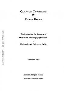
Figure 1.1. (a) Graphical representation of a generic monodimensional Bloch-wavefunction Ψn,k (x) = un,k (x) eik·x and its components: the slowly oscillating plane wave eik·x and the latticeperiod function un,k (x). Grey dots are crystal nuclei and U (x) is the relative 1D lattice periodic potential (Kronig-Penney). (b) Energy bands formation in a tetrahedral crystal cell (Si or Ge): as one can see from the plot representing the transformation of electronic energy levels as a function of the interatomic distance, orbitals may overlap and degenerate into bands which open at the equilibrium radius a0 determining a typical forbidden gap Eg = EC − EV .

The first observation about Eq. (1.1) is that the wavefunction Ψn,k (r) cannot be any possible function but it must be eigensolution of the (time-independent) Schrödinger equation ~2 ∆r Ψn,k (r) + U (r)Ψn,k (r) = En (k)Ψn,k (r) , 2m∗ where ~ is the reduced Plank constant, m∗ the carrier effective mass, −

~2 k2 with n = 1, 2, 3, . . . 2m∗ (n is the principal quantum number of the state/sub-band) and En (k) ' En +

(1.2)

(1.3)

~2 ∆r (r) + U (r) (1.4) 2m∗ is the Hamiltonian operator of the system. The other important consideration has to do with the presence of the subscript k, and consists in the fact that we can find a completely different solution of Eq. (1.1) by changing the wavevector k: the wavevector here becomes a true quantum number, labeling in Eq. (1.2) the complete basis of Bloch-wavefunctions. As a consequence of the Bloch theorem, also energy eigenvalues are periodic as Ψn,k (x) in the reciprocal lattice, so: H=−

En (k + K) = En (k) .

8

(1.5)


a)

b) z x

.. . E4 (k) E3 (k)

conduction band

y

En (k)

π a0

− aπ0 valence band

a0

E2 (k)

kx,y,z E1 (k)

c


Figure 1.2. (a) Simplified 2D representation of a periodic cubic crystal, where the lattice parameter a0 is highlighted. (b) Corresponding band structure of a direct band gap material in the first Brillouin zone (FBZ), i.e. for |k| ≤ aπ0 , where k is the crystal wavevector k projected along one of the three axes of the real space. First conduction and valence band states En (k) around the Γ symmetry point (k = 0) are also represented, while the grey area is the band gap.

These results represent a remarkable difference from what one can observe in free atoms, where the electronic potential of nuclei determine a well-defined spectrum of energy levels and wavefunctions, whatever the value k. In case of solids, valence electrons are seen as an ensemble of fermions whose wavefunction is represented by a term un,k (r) with the same period of lattice potential (Kronig-Penney potential [1]) modulated by a slowly oscillating plane wave eik·r . The energy spectrum now depends on the lattice momentum ~k and is no more a set of discrete spectrum of possible states but the orbital levels result to be degenerated into a system of allowed (or forbidden) “bands”, where states are energetically dense. When k assumes real values the band is allowed, otherwise we are in presence of forbidden states, since there the eigenfunctions are exponentially decaying. The framework we developed is at the basis of the energy band theory, a formalism merging quantum mechanics and solid-state physics in a unique model which is able to predict the behavior of electrons in a periodic crystal. Now we have the fundamental elements to investigate the energy structure of each solid. What makes the difference between a descriptive model and another one is the way of approximating the lattice potential (see, for instance, the virtual-crystal approximation in Section 2.2.2). Rigorous approaches consist in the tight-binding approximation and the k · p perturbation method : the first one describes the system accounting for atomic orbitals of only nearby atoms, and the second one is based on an Hamiltonian with perturbation terms in the momentum space. Before entering in the details of this last method, let us start from the bands formation (see panel

9


(b) in Figure 1.1). Typically, in direct band gap semiconductors, atoms are connected through σ-bonds, consisting in a superposition of p-orbitals in a three-fold sp 3 hybridization (p-lobes are lying on all the three directions of the real space: p x , p y , p z ). These bonds give the major contribution to the shape of un,k (r) and the related probability density |un,k (r)2 | while, at the same time, they are responsible for the differentiation of valence electrons in at least three sub-bands. Moreover, if we include also spin-orbit interactions, that is the overlapping term (s × L) of interaction between the intrinsic electron angular momentum (i.e. the spin s) and the magnetic field generated by the nuclei (or their momentum L, almost equal to the electron orbit momentum), the energy splitting becomes even more evident. Similarly, for what concerns conduction states, the s-orbitals and their quasispherical symmetry dominate the shape of the rapidly oscillating part of the wavefuction. Thanks to this symmetry, the formation of a conduction band could be explained solely through the overlap/degeneration of s-orbitals, without accounting for any sub-band splitting effect, as we did instead for valence band. Nevertheless, the lack of orbital momentum L in s-states does not allow spin-orbit effects. The only possible degeneration, at this stage of approximation, could be a slight contribution of the p-orbital to the conduction band at high energies (see, again, panel (b) in Figure 1.1). But as long as we assume L ' 0 the sp two-fold splitting in this case will be considered negligible. As we may appreciate from Figure 1.2, panel (b), in direct band gap semiconductors like Hg1−x Cdx Te, GaN, Inx Ga1−x N or Alx Ga1−x N the conduction band (CB) minimum and the top of the valence band (VB) are located at the critical point Γ of the first Brillouin zone (FBZ), i.e. at k = 0. This represents an advantage for some kinds of applications, especially in optoelectronics, where the most probable part of direct transitions between CB and VB can be established without interactions in the momentum space (∆k = 0), as instead occurs in phonon-assisted processes. Being the conduction and valence band trend almost parabolic in k (see again panel (b) in Figure 1.2 and also Eq. (1.3)), if we neglect the tensorial notation for carrier effective masses around Γ, then one can see that m∗ can be considered proportional to the curvature of the function E(k). In fact: 1 d2 En (k) 1 ' 2 . m∗ ~ dk2

(1.6)

The lower the concavity, the higher m∗ . Now we briefly derive the k · p formalism starting from the substitution of a generic Bloch-wavefunction into the Schrödinger equation: ~2 ~ ~2 k2 − ∗ ∆r + ∗ k · p + + U (r) un,k (r) = En (k) un,k (r) (1.7) 2m m 2m∗ where p = −i~∆ is the momentum operator. Supposing to know the Hamiltonian and the wavefunction at a given k0 Hk0 = −

~2 2 ~ ~2 k20 ∇ + k · p + + U (r) 0 2m∗ r m∗ 2m∗

10

(1.8)

1.2 Carrier Statistics

and Ψn,k0 (r) = un,k0 (r) eik0 ·r , then Eq. (1.2) becomes ~ ~2 2 2 Hk0 + ∗ (k − k0 ) · p + (k − k0 ) un,k0 (r) = En (k) un,k0 (r) , m 2m∗

(1.9)

(1.10)

where un,k0 (r) =

X n0

An0 ,n (|k − k0 |) un0 ,k0 (r) ,

(1.11)

If we plug Eq. (1.11) into Eq. (1.10), after multiplying both sides by u∗n,k0 (r) and integrating over the volume of a unit cell, we obtain the eigenvalue secular equation: X ~2 ~ 2 2 En (k0 ) + (k − k0 ) δn0 ,n + ∗ (k − k0 ) · pn0 ,n An0 ,n = En (k) An,n ∗ 2m m 0 n (1.12) in which m~∗ (k − k0 ) · pn0 ,n is our perturbation term and where Z pn0 ,n = u∗n,k0 (r) p u∗n0 ,k0 (r) dr . (1.13) Now one can proceed to solve the k · p secular equation written for k ' k0 , determining the coefficients An0 ,n and then also the eigenvalues En (k) of the system in the perturbation framework. As we shall see in next chapters, the most important transitions in direct band gap semiconductors involve the main conduction band (CB) and at least three valence bands, depending on the effective hole mass m∗h : so we have the heavy hole (HH) band, the light hole (LH) band and the split-off (SO) band. The presence of three different valence bands is due to the state separation produced, in turn, by spin-orbit interaction effects, since otherwise they would be degenerate.

1.2

Carrier Statistics

The classical picture describing a charge population in solids and its related density is usually based on the Fermi-Dirac statistical distributions 1

fFD (E) = e

E−EF kB T

,

(1.14)

+1

with kB the Boltzmann constant and EF the Fermi energy, which represents the highest possible energy of carriers when T = 0. This formalism is straightforward for electrons, which are fermions (1/2-spin particles obeying to the Pauli exclusion principle) and, by symmetry, is also applied to holes. Now, differential carrier densities are given by ( dn = ρC (E) fFD (E) dE , (1.15) dp = ρV (E) (1 − fFD (E)) dE

11

ρC (E)

energy

energy

energy

1.2 Carrier Statistics

1 − f (E)

EF −EC

n = NC e kB T = ρC (E) f (E)

EC

EC

EC

EF

EF

EF

EV

EV

EV

ρV (E)

0.5

density of states

EV −EF

f (E) 1

p = NV e kB T = ρV (E) (1 − f (E))

Fermi function

carrier density

c


Figure 1.3. Density of states (DOS), Fermi function and carrier density represented as a function of energy in intrinsic semiconductors (EF ' (EV +EC )/2 and n = p = ni at equilibrium) for T > 0.

where ρC (E) and ρV (E) are the so-called density of states (DOS)  √ dNC (E) 4π 8m∗e p   = E − EC , for E ≥ EC ρC (E) = dE h p ,  4π 8m∗h p dN (E) V  ρV (E) = = EV − E , for E ≤ EV dE h

(1.16)

which indicate how many states (occupied or not) can be found for a given energy E, and where NC (E) and NV (E) are the effective densities in conduction and valence band ∗ 3 me,h kB T 2 NC,V = 2 , (1.17) 2π~2 where m∗e,h is the electron/hole effective mass. At T = 0 the function fFD (E) is a step-function such that ( 1 if E ≤ EF fFD = 0 if E > EF

(1.18)

while, as represented in Figure 1.3 for a generic intrinsic semiconductor, when T is greather than zero the Fermi-Dirac distribution function becomes smoothed in a region approximately wide ∼kB T . This implies that only at thermal equilibrium (T = 0) EF represents the energy which corresponds to completely filled VB and empty CB. At higher temperatures we have that f (EF ) = 1/2. So, if EF stays within the band gap (i.e. for low doping densities) and the energy gap is sufficiently greater than kB T , then the semiconductor can be still considered somehow at thermodynamic equilibrium. If the gap is narrower, instead, the finite probability fFD (E) to

12

1.3 Doping and Carrier Concentrations

have an electron in CB (and, at the same time, the probability (1 − f (E)) to have a hole in VB) can induce “spontaneous” band-to-band transitions typical of these materials, as we will see talking about tunneling phenomena. The Fermi-Dirac distribution is not only valid for intrinsic semiconductors, i.e. the one in which the Fermi level equals the intrinsic one NV 1 (EC + EV ) + kB T log , (1.19) EF ≡ EFi = 2 NC but it can be also applied to other materials like degenerate semiconductors, where doping levels are very high. Nonetheless, the choice of an approximated description is common when we study non-degenerate materials. This approximation consists in using the Boltzmann distribution function fB (E) = e

−

E−EF kB T

(1.20)

in place of fFD , where now the carrier population no longer obeys to the Pauli exclusion principle. Comparing the two formulations one can notice that E − EF 1, (1.21) fFD (E) ' fB (E) ⇔ exp kB T i.e. for E kB T . At this limit the classical Boltzmann treatment in place of the semiclassical Fermi-Dirac one is rather well acceptable. Finally, integrating the differential density for electrons and holes in Eq. (1.15) with respect to the bands we obtain their concentrations at equilibrium:  E −E n = N e FkB T C C , (1.22) EV −EF  kB T p = NV e where np =

E p − g NC NV e 2kB T ≡ ni .

(1.23)

Alternatively, one can also write  EF −EF n = n e kB T i i . EF −EF i  kB T p = ni e

1.3

(1.24)

Doping and Carrier Concentrations

A building-block of each solid-state system is constituted by the feature of artificially enhance the native carrier concentrations through the introduction of impurity atoms. These dopants elements may act as donors or acceptors and their energy ED or EA tipically lies just below the CB minimum or above the top of the VB,

13

1.4 Generation/Recombination Mechanisms

respectively. The difference between this energy and the corresponding band edge is called ionization energy Eion : ED,ion = EC − ED

or EA,ion = EA − EV .

(1.25)

In neutral conditions the new Fermi level due to doping is determined by the balance equation ntot = n + nD = p + pA = ptot (1.26) where the ionized carrier densities, still obeying to the Fermi statistics, are  1  nD = ND EF −ED   kB T 1 + gD e , (1.27) 1   p = N  A EA −EF  A 1 + gA e kB T being gD and gA the degeneracy factors (usually gD = 2 and gA = 4). Eq. (1.27) is known as the incomplete ionization law, since nD and pA determine the fraction of thermally ionized dopant, once their nominal values ND and NA are given. In other words, effective doping can reach the concentration of implanted chemical dopants only in the limit of high T , so: ( T →∞ nD = ND . (1.28) T →∞ pA = NA When a doped semiconductor is out of equilibrium (by carrier injection or other external stimuli), the Fermi level changes its position going close to the CB in n-type materials and to the VB in p-type ones: ( EFn = EFi + kB T ln (ntot /ni ) . (1.29) EFp = EFi − kB T ln (ptot /ni ) These two new energies are called quasi-Fermi levels.

1.4

Generation/Recombination Mechanisms

The usual operation state of semiconductor-based electronic devices consists in a non-equilibrium condition. In this regime the external energy given to the system is partially converted into a signal (optical or electrical) through specific transitions which can take place in the energy domain, as well as in real or momentum space. In the case of direct band gap semiconductors, most of the common transitions between bands occur at the Γ symmetry point, where the gap reaches its minimum energy, Eg . This is the condition in which electron/hole pairs are generated or recombined (annihilated), depending on whether the energy is absorbed or delivered, respectively. This energy can involve a photon, i.e. a quantum of light, as in case of

14


optical processes. But, in general, interband transitions may occur also in the nonradiative regime. Generation/recombination mechanisms change the availability of carriers in CB and VB, both majority and minority, determining relaxation processes towards equilibrium which can affect and limit the device performance by means of carriers lifetime enhancement. So, GR processes can be divided into two main categories, non-radiative and radiative mechanisms. In both, generation consists of an electron coming from CB that occupies an empty state (hole) in VB, while recombination is its inverse, and these two competitive processes are perfectly balanced at equilibrium. Electron/hole pairs are generated or recombined through a characteristic lifetime, depending on the material and on the particular GR mechanism involved. Out of equilibrium the algebraic sum of the generation G and recombination R rate is the so-called net generation/recombination rate U = G − R, i.e. the number of pairs recombined per volume in the unit time (cm−3 s−1 ), which is a function of the carrier densities at equilibrium n0 , p0 and out of equilibrium n0 , p0 such that U 6= 0 if and only if ∆n 6= 0 and ∆p 6= 0, where ∆n = n0 − n0 and ∆p = p0 − p0 . This set of properties goes under the name of relaxation time approximation, according to which we have:  ∆n n0 − n0   = U '  n τn τn , 0 p − p0 ∆p   U p ' = τp τp

(1.30)

where τn and τp are the electron and hole lifetimes, respectively. For small excess carrier concentrations ∆n, ∆p and within the Boltzmann statistics framework:  ∆n ∂∆n   '−  ∂t τn (1.31) ∂∆p ∆p   '−  ∂t τp that yields: ( n(t) = ∆n e−t/τn + n0 , (1.32) p(t) = ∆p e−t/τp + p0 from which it is even more clear why τ are called relaxation times, being the time constant needed to restore the original equilibrium concentrations n0 , p0 . Under the same assumptions given before, the lifetime contribution coming from each GR process (non-radiative, radiative and others) can be treated as independent. For this reason: X 1 1 = (1.33) τtot τj j where index j stands for the contribution from a j -th GR process.

15


EC

Etrap

EV a)

b)

c)

d)

c


Figure 1.4. Single-level model of Shockley-Read-Hall (SRH) generation and recombination processes in a direct band gap semiconductor. Solid arrows represent: (a) electron capture. (b) electron emission. (c) hole capture. (d) hole emission. Completing the processes with dashed arrows we have recombination in (a) and (c) and generation in (b) and (d).

1.4.1

Non-radiative mechanisms

1.4.1.1

SRH generation/recombination

A first class of non-radiative processes involves a certain density Ntrap of energy levels within the semiconductor band gap, like dopants, impurities or defects. These states, also called Shockley-Read-Hall (SRH) centers, can assist interband transitions which are typically stimulated by energies lower than Eg . As depicted in Figure 1.4 for a single-level model, these transitions may follow four different channels. In panel (a) an empty SRH trap (with and energy Etrap ) is occupied by a conduction electron with capture cross-section σn and capture rate cn = σn vthn , where vthn is the thermal speed of the electron. In (b) an electron escapes from a trap with emission rate en and is promoted into CB. Panels (c) and (d), instead, respectively represent the capture and emission of a valence hole with rates cp = σp vthp and ep . Likewise, vthp is the thermal speed of the hole and: s vthn,p =

3kB T . m∗e,h

(1.34)

Deriving Eqs. (1.32) with respect to time and recalling Eq. (1.30), which is valid for small ∆n and ∆p, one can write the time-evolution of carriers in SRH processes

16


for direct band gap semiconductors as [2]  dn(t)  USRHn = − = −cn n(t) Ntrap (1 − ftrap (Etrap )) + en Ntrap ftrap (Etrap ) dt (1.35)  dp(t) U = −cp p(t) Ntrap ftrap (Etrap ) + ep Ntrap (1 − ftrap (Etrap )) SRHp = − dt that, thanks to the charge neutrality law, are linked via n(t) + Ntrap ftrap (Etrap ) = p(t) ,

(1.36)

where ftrap (Etrap ) is the occupation function of the trap level. At steady-state equilibrium (i.e. when dn = 0, dp = 0, n ≡ n0 and p ≡ p0 ): dt dt  Etrap −EF i en0  kB T  = n e ≡ n1 i c n0 EF −Etrap i e    p 0 = ni e k B T ≡ p1 cp0

(1.37)

and 1 1 = cn Ntrap σn vthn Ntrap , 1 1 = = cp Ntrap σp vthp Ntrap

   τn0 =   τp0

(1.38)

where n1 and p1 are valid when Etrap ≡ EF . ± Now, assuming Ntrap = Ntrap ftrap (Etrap ) the fraction of occupied (charged) traps 0 and Ntrap = Ntrap (1−ftrap (Etrap )) the same quantity referred to unoccupied (neutral) ones, we can rewrite Eq. (1.35) as  dn(t) 0 ±   = −cn (n Ntrap − n1 Ntrap ) dt . (1.39)   dp(t) = −c (p N ± − p N 0 ) p 1 trap trap dt Then we have (still in steady-state conditions) that ± dNtrap dn(t) dp(t) = − + dt dt dt 0 ± ± 0 = cn (n Ntrap − n1 Ntrap ) − cp (p Ntrap − p1 Ntrap )

which must be null by definition (except for transient regimes). Thus:  cn n 1 + cp p 0   Ntrap = Ntrap c (n + n ) + c (p + p ) n 1 p 1 . c n + c p n p 1  ±  N = N  trap trap cn (n + n1 ) + cp (p + p1 )

17

(1.40)

(1.41)


By using all the previous relations, the relaxation process involving excited carrier densities n0 , p0 can be written as dn0 (t) dp0 (t) (n0 + ∆n) (p0 + ∆p) − n2i = = = USRH . dt dt τp0 (n0 + ∆n + n1 ) + τn0 (p0 + ∆p + p1 )

(1.42)

So, for electrons: −1 dn0 = − ∆n dt τp (n0 + ∆n + n1 ) + τn0 (p0 + ∆p + p1 ) ∆n = − 0 (n0 + ∆n) (p0 + ∆p) − n2i σn vthn (n0 + ∆n + n1 ) + σp vthp (p0 + ∆p + p1 ) = − ∆n 2 σn vthn σp vthp Ntrap [(n0 + ∆n) (p0 + ∆p) − n2i ]

(1.44)

np − γn γp n2i EF −Etrap Etrap −EF i i kB T kB T + τn p + γp ni e τp n + γn ni e

(1.46)

τSRHn

(1.43)

(1.45)

and similarly for the holes. Then, recovering our previous steady-state assumptions: USRH =

(from which is evident that USRH is maximized when Etrap = EFi ) and 1 τSRHn,p = , σn,p vthn,p Ntrap

(1.47)

where the functions γn,p are equal to 1 in case of Boltzmann statistics (as supposed so far) otherwise, in the Fermi statistics picture  C n − EFkn −E   BT γ = e  n NC (1.48) p − EVk−ETFp   B γp = e NV and the carrier densities become  EFn − EC   nF = NC F1/2 kB T , (1.49) EV − EFp   pF = NV F1/2 kB T where NC,V are the conduction/valence band effective densities, F1/2 () represents the 1/2-th order Fermi integral Z∞ √ 2 E F1/2 () = √ dE (1.50) 1 + eE+ π 0

and EFn,p are the quasi-Fermi levels for electrons and holes, which generate from the Fermi level when the material is out of equilibrium. Now, since τn = ∆n/USRH and τp = ∆p/USRH , as stated by Eq. (1.43), by using one of the possible representations of carrier densities (Boltzmann or Fermi) one can appreciate the T -dependence of the SRH rate, which is increasing with temperature.

18


1.4.1.2

Auger generation/recombination

Besides defect-assisted non-radiative GR processes, a very important family of processes is represented by Auger mechanisms, “three-body” interactions classified depending on which carriers or sub-bands are involved. So, in principle, different types of Auger GR can exist. The most important are depicted in Figure 1.5: in panel (a) we find the “eeh” transition, which is the recombination of a CB electron, where the excess energy is released to a second electron that can be promoted to a higher conduction level; then in (b) the “ehh” process is represented, where the energy is released to a hole, contrarily to the previous case; finally (c) represents the “hhe” generation due to a hole promoted into the CB, where the excess energy is transferred to another hole that is excited into a deeper valence state. As just mentioned, processes (a) and (b) involve the recombination of an electron/hole pair before interacting with a third carrier. The case (c), instead, represents an example of Auger generation, a process which is commonly referred to as impact ionization. In this sense Auger and impact ionization are symmetric processes, whatever the kind of carriers involved. If Auger GR can be heavily present in forward-biased light-emitting diodes based on wide band gap materials, especially at high T or injection regimes, impact ionization can be more important in narrow band gap IR photodiodes, which operate in reverse bias conditions. Being a three-body mechanism, the net Auger recombination rate is fundamentally different from traditional non-radiative rates. Moreover one has to observe that its rate roughly goes like ∼n2 p for “eeh” processes or ∼np2 for “ehh” ones and, in general, it is proportional to the third power of the total carrier density or, in turn, to the doping level. Now we go through the derivation of a macroscopic description of the Auger recombination rate and lifetime, starting from quantum theory based on microscopic quantities towards the common expressions used in experimental or modeling studies. To do this, a formalism among all those present in the literature has been chosen, which is the one developed by P. T. Landsberg and well discussed in Ref. [3]. Let us start with considering as a template example the process CHCC. A new detailed scheme is proposed in Figure 1.6, where all the single steps constituting the whole process are highlighted and properly labeled: numbers 1 and 10 indicate respectively the initial and the final states of the first “direct transition”, i.e. the band-to-band recombination of an electron/hole pair, while 2 and 20 are the initial and final state of the second process, which we shall call “exchange interaction”. In the Landsberg formalism they are all described by Bloch states. So, by using the Fermi golden rule in the first-order perturbation theory, the overall transition rate as a function of time t can be written as 2πt (1) 2 (0) (0) 0 , (1.51) |W1→2 (t)| = H20 →1 δ E20 − E1 ~ (1)

where H20 →1 is the first-order perturbed interaction Hamiltonian while energies at (0) (0) the initial and final state E1 , E20 are evaluated as zero-th order (non-perturbed) (1) (1)∗ terms. Notice that H (1) is time-independent and also Hermitian, so H20 →1 ≡ H1→20 .

19


EC

EV b0 ) a)

b)

c)

c


Figure 1.5. Most important Auger generation/recombination processes in a direct band gap semiconductor (without any phonon- or defect-assisted mechanism). (a) “eeh” Auger recombination also named CHCC where, after the electron/hole has recombined, a second electron is excited. (b) “ehh” Auger recombination, or CHHL, in which the same recombination is followed by a transition involving a hole. Process (b0 ) is only a slight variant of the previous one and is labeled as CHLH. (c) “hhe” Auger generation (or, better, impact ionization) where, after the electron/hole pair generation, a second hole is promoted to another valence energy state. Notice that this scheme also includes the third carrier participating to the GR transition, here represented by filled/empty grey dots, respectively for electrons and holes.

Moreover: (1) 2 H 20 →1 = 2 β |Md |2 + |Me |2 ,

(1.52)

where β is a spin-related term such that 1 < β < 2 while Md and Me are the Bloch matrix elements for direct and exchange transition, respectively. It can be demonstrated that they can be approximated as |Md | '

4πq 2 |F1,2 F10 ,20 | δk +k , k +k V λ2 + |k1 − k10 |2 1 2 10 20

(1.53)

|Me | '

4πq 2 |F1,20 F10 ,2 | δk +k , k +k , V λ2 + |k2 − k10 |2 1 2 10 20

(1.54)

and

in which q is the elementary charge, and V are the material dielectric constant and volume, respectively, λ−1 is the Coulomb screening radius, the four F represent all the possible Bloch wavefunction overlaps and k1 , k10 , k2 and k20 are the momenta corresponding to the states involved in the “eeh” process (see Figure 1.6). Putting together the equations we reported, the interaction Hamiltonian can be

20


E(k)

conduction band

2’

“exchange”

CHCC Auger recombination

1 “direct”

k10

2

band gap k1

k2

k20

k

valence band

1’

c


Figure 1.6. CHCC Auger (“eeh”) recombination process, where the four Bloch states and their momenta have been labeled. The first “direct” transition corresponds to the electron/hole recombination while the subsequent “exchange” interaction due to momentum conservation consists of an excitation of a second electron within the conduction band (CB).

rewritten as follows: ( 32π 2 q 4 |F1,2 F10 ,20 |2 |F1,20 F10 ,2 |2 (1) 2 H20 →1 ' 2 + 2 2 V 2 λ2 + |k1 − k10 |2 λ2 + |k2 − k10 |2 2 ) 0 F10 ,2 0 ,20 F F F 1,2 1,2 1 − δk1+k2 , k10 +k20 . (1.55) + λ2 + |k1 − k10 |2 λ2 + |k2 − k10 |2 Now the CHCC Auger recombination probability per unit volume and per unit time is given by: Z 2t (1) 2 1 − cos x P ' 2 Φ H20 →1 dk1 dk2 dk10 dk20 ~V x2 3 Z 32π 2 q 4 t ∆n ∆p V ' + f (1) f (2) (1 − f (10 )) (1 − f (20 )) V 3 ~2 3 n0 p0 8π 3 EF −EF 1 − cos x − nk T p B × {· · · } 1 − e dk1 dk2 dk10 dk20 (1.56) x2 where Φ is computed at equilibrium as 0

0

Φ = f (1) f (2) (1 − f (1 )) (1 − f (2 ))

−

1−e

EF −EF n p kB T

,

in which the f ’s are the Fermi-Dirac occupation functions, and where t (0) (0) x= E20 − E1 . ~

21

(1.57)

(1.58)


The term omitted for reasons of brevity in Eq. (1.56) is the same within braces in Eq. (1.55). If one notices that the total CHCC recombination probability is intrinsically dominated by the “direct” process, then the bracketed term can be reduced to the only first addend. At this point, lifetimes and recombination rate of any Auger process can be computed from the CHCC probability P through 1 1 1 = + τA τn,A τp,A P P = + n − n0 p − p0 p(np − n0 p0 ) n(np − n0 p0 ) + Cp = Cn ∆n ∆p Cn n Cp p ' + (np − n2i ) , ∆n ∆p

(1.59)

in which the last equality becomes exact for intrinsic semiconductors. From lifetimes, as usual, we can derive the recombination rate in equilibrium conditions (∆n = ∆p) remembering that R = ∆n/τ . So: RA = (Cn n + Cp p) (np − n2i ) .

(1.60)

Coefficients Cn,p represent a macroscopic (and somehow semi-empirical) description of the many-body theoretical probability integral P . They are material and process dependent and are expressed in cm6 s−1 units.

1.4.2

Radiative mechanisms

The last important category of GR processes is represented by radiative mechanisms. They are essential in optoelectronics since (spontaneous) radiative recombination is the building-block physical mechanism in light-emitters and photogeneration, its symmetrical process, is at the basis of light detection. Discarding at this moment all tunneling or trap-assisted transitions, one can say that the simplest way to define radiative GR is that they are processes where the excess energy released (absorbed) during the band-to-band transition is given to (by) a photon, as schematically reproduced in Figure 1.7. Due to the finite probability of having optical transitions at k > 0, usually the emission spectrum of a given semiconductor does not coincide with a δ-Dirac function but it corresponds to a broad curve, typically modeled by a Lorentian as L(ν) =

1 Γ (ν) , 2π (Eg − 2π~ν + ~ν)2 + (Γ (ν)/2)2

(1.61)

where Γ (ν) is a Gamma function of the photon energy Eph = hν. Now we re-propose here a very short derivation of the radiative recombination rate Rrad from quantum principles, which finds its origins in the k · p method.

22


E(k)

conduction band

hν1 = Eg

hν2 > Eg

EC − EV = Eg

k valence band

c


Figure 1.7. Simplified representation of spontaneous radiative recombination with photon emission at different energies and, thus, involving states with different wavevectors: for transitions at the symmetry point Γ (i.e. k = 0) the photon energy hν exactly corresponds to the energy gap Eg otherwise, at higher wavevectors, must be hν2 > Eg .

Again we exploit the Fermi golden rule to write the recombination rate probability in multi-photon emission mode, which is [3] Prad (E, νk ) =

X 4q 2 n ˆ νk |Mi,f (k)|2 δ (Ei − Ef − ~νk ) (Nk + 1) , 2 V c3 ~2 m ¯ i,f

(1.62)

where “i” and “f” label the initial and final state in conduction and valence band, respectively, ~νk is the k-dependent photon energy, Nk the number of emitted photons per each k point, c is the speed of light in vacuum, V the material volume, n ˆ its refractive index, m ¯ = m∗C |m∗HH | / (m∗C + |m∗HH |) and Mi,f is the transition matrix element 2

2

|Mi,f (k)| = Pi,f |Fi,f (k)|

m0 Eg (Eg + ∆SO ) m∗C (k) , −1 m0 12 Eg + 23 ∆SO

(1.63)

being Pi,f a polarization term (due to spontaneous piezoelectric charges induced by lattice bond potentials), ∆SO is the spin-orbit splitting energy responsible for the gap between HH/LH bands and the SO band in Γ and, finally, Fi,f is the wavefunction overlap integral of conduction/valence band states involved in the radiative transition. The expression which describes the probability rate is k- and E-dependent, so (as we published in the paper of Ref. [4]) we can obtain the total net recombination

23

1.5 Classical Transport in Semiconductors

rate by integrating it over all the possible wavevectors and energies: ZZ Rrad = Prad (E, νk ) dk dE X Z Z 4q 2 n ˆ νk = |Mi,f (k)|2 f (Ef ) (1 − f (Ei )) L(νk ) k dk dE (1.64) 2 3 2 m Vc ~ i,f where f are the Fermi-Dirac functions and L(νk ) is the wavevector-dependent Lorentian broadening. Again, as well as for Auger processes, even the rate in Eq. (1.64) can be modeled via an empirical point of view. The typical simplified description is Rrad ' B (n0 + ∆n) (p0 + ∆p) = Bnp ,

(1.65)

being B, also called ‘bi-molecular’ coefficient, a material dependent parameter (in cm3 s−1 ). The second equality in Eq. (1.65) is valid for intrinsic semiconductors. In these conditions ni ni = , (1.66) τi,rad = 2Rrad 2Bnp from which the radiative lifetime at equilibrium τrad =

2ni τi,rad . n+p

(1.67)

−1 Coefficients A = τSRH , Brad and Cn,p define the so-called “ABC model” describing GR processes in semiconductors.

1.5

Classical Transport in Semiconductors

In order to describe electrical/optical operation of semiconductor devices and to model them the knowledge about carriers dynamics is essential. In addition, device simulation isn’t only a strategy to predict specific structure behaviors, but it also represents today’s workbench for investigating advanced device performances. Although solving the electrical problem may constitute a formidable mathematical challenge – especially in three-dimensional (3D) simulations – it is possible to simplify the real physics by modeling only the dynamic description of locally averaged variables through approximated solutions of opportune partial differential equations (PDEs). Such average values are obtained thanks to a geometrical discretization method, like the finite element (FEM), finite boxes (FB) or finite volume (FVM). These spatial discretization schemes allow to reduce the PDE equations to a discrete system of ordinary differential equations (ODEs) that it is possible to linearize under specific theoretical hypotheses. In the present chapter we analyzed some of the most important GR mechanisms. Moreover, in Chapter 4 direct (BTBT) and defect-assisted tunneling (TAT) models

24


designed for physics-based numerical simulation of optoelectronic devices will be treated and finally expressed through opportune rates (number of carriers which tunnel per volume per second). These rates may correspond to generation rates, in case of BTBT in narrow band gap reverse biased diodes, or recombination rates, as for TAT in wide band gap forward biased junctions. This section has the purpose to clarify the framework in which both standard GR and such tunneling rates play and how they can enter into device-level numerical simulation.

1.5.1

Short recall about drift-diffusion (DD) model

The simpler starting point in semiconductor transport theory is represented by the Poisson equation, given by the PDE ∇2r φ(r)

qφ(r) − χ(r) − Eg (r) q = − ND (r) − NA (r) + NV (r) exp kB T ! −qφ(r) − χ(r) − NC (r) exp , (1.68) kB T

where φ is the electrostatic potential, the dielectric constant, ND , NA , NV and NC are, respectively, the concentrations of donors and acceptors and the effective densities in valence and conduction band, χ is the electron affinity and q the elementary charge. Note that Eq. (1.68) is written in its most generic form since all the possible spatial dependencies have been made explicit. By introducing now the Boltzmann statistics we have carrier distribution functions f (k, r, t) that must obey the so-called Boltzmann transport equation (BTE): F df (k, r, t) ∂f (k, r, t) + v(k) · ∇r f (k, r, t) + · ∇k f (k, r, t) = (1.69) ∂t ~ dt coll where v(k) is a group velocity and F is the specific force field acting on the particles constituting our system, such that F = ~(dk/dt). The left-hand side expression represents a drift term while (df /dt)|coll is a collision term. Furthermore, under relaxation time approximation (see Section 1.4): df (k, r, t) |f (k, r, t) − f0 (k)| =− , (1.70) dt τ (k) coll where f0 (k) refers to thermodynamic equilibrium. Once the acting field is set, there are several techniques to solve the BTE. One of these is the Hydrodynamic (HD) model, suitable for systems with many electron-electron scattering events, like in submicrometric and micrometric devices, heterostructures or quantum wells. Its unknowns are the carrier concentrations n and p, their energy E and the electrostatic potential φ. Besides HD we find the Drift-Diffusion (DD) model, used in the analysis of micrometric devices (down to

25


0.5 µm) in diffusive transport regime, by self-consistently solving Eq. (1.68) and the continuity equations for electron/hole current densities Jn,p (r, t)  ∂n(r, t) 1   = + ∇r Jn (r, t) − Un (r, t)  ∂t q , (1.71)  ∂p(r, t) 1   = − ∇r Jp (r, t) − Up (r, t) ∂t q where U (r, t) = G(r, t) − R(r, t) is the net generation/recombination rate, i.e. the algebraic summation of terms G and R, and current densities are  Jn (r, t)   = Dn ∇r n(r, t) − µn (∇r φ(r, t)) n(r, t)  q , (1.72)  Jp (r, t)   = Dp ∇r p(r, t) − µp (∇r φ(r, t)) p(r, t) q where Dn,p are the diffusion coefficients and µn,p =

drift drift vn,p vn,p =− E ∇r φ(r, t)

(1.73)

the electron/hole mobilities. The DD model is valid under the assumption according to which field variations produce in all the unknowns – n(r, t), p(r, t) and φ(r, t) – slower changes with respect to the energy relaxation time of the system τ . A formal link between BTE and DD model can be established through the so-called method of moments, according to which the generalized statistical moment is computed by integrating in the k-space Eq. (1.69) multiplied by λ, an opportune function of k: Z Z Z Z df ∂ F (1.74) λ f dk + ∇r v(k) λ f dk − ∇k λ f dk = λ dk , ∂t ~ dt coll k

k

k

k

where f = f (k, r, t) and assuming λ = λ(k) =

N X

a j kj

j=0

with

= a0 + a1 k + a2 k2 + . . .

(1.75)

 a0 = 1        a1 = ~ k ~2 k2 .  a2 =   2 m∗e     ..  .

(1.76)

26


Now we are able to define Z Mj =

λj (k) f (k, r, t) dk

(1.77)

k

as the so-called j-th order moment of f (k, r, t). So one can see that the first three moments correspond, respectively, to the carrier concentration, the carrier average momentum and the carrier average energy. In particular, by using Z M0 = f (k, r, t) dk = n(r, t) (1.78) k

into Eq. (1.69) one can obtain the charge conservation law for electrons ∂n(r, t) dn(r, t) + ∇r (¯ vn n(r, t)) = , ∂t dt coll

(1.79)

Jn = −q v¯n n(r, t)

(1.80)

dn(r, t) = −Un (r, t) , dt coll

(1.81)

that, being and

coincides with the electron continuity equation, where R v(k) f (k, r, t) dk k v¯n = R f (k, r, t) dk

(1.82)

k

is the average electron velocity. Now notice that Eq. (1.71) states that each carrier is characterized by a conservation law where the outgoing charge in the transport term ∇r Jn,p is (fully or partially) balanced by the generation/recombination contribute Un,p . Not only electrons and holes obey this conservation principle but also fixed charges – like defects or dopants – do so, even if they don’t have a transport counterpart at play. Defining the effective concentration of these level k as ( + ND,k (r, t) for donors ± (1.83) Ck (r, t) = − −NA,k (r, t) for acceptors we can write the corresponding continuity equation ∂Ck± (r, t) X + Un,k (r, t) − Up,k (r, t) = 0 ∂t k

27

(1.84)


The final set of DD equations, in a 3D time-variant framework, is  ∂n(r, t)   = −∇ n(r, t) µ ∇ φ(r, t) − D ∇ n(r, t) − Un (r, t)  n r n r  ∂t      ∂p(r, t)    = ∇ p(r, t) µ ∇ φ(r, t) + D ∇ p(r, t) − Up (r, t) p r p r  ∂t , ± X  ∂C (r, t)  k  + Un,k (r, t) − Up,k (r, t) = 0    ∂t  k      ∇2 φ(r, t) = − ρ(r, t) r

(1.85)

where the overall charge density ρ has become ! ρ(r, t) = q p(r, t) − n(r, t) +

X

Ck± (r, t)

(1.86)

k

and where all generation/recombination (and tunneling) mechanisms we discussed in the present chapter can enter by means of their G or R rate.

1.5.2

Boundary conditions

In this subsection we deal with the solution of PDEs which constitute the system (1.85), starting with a suitable ensemble of initial conditions (IC) and boundary conditions (BC), then by applying a certain spatial discretization allowing to reduce the PDE complexity. Typically, the IC stem from the specific physical problem one has to solve, whereas BC are quite standard in numerical simulations and deserve special attention as well as the GR models included into the continuity equation. These conditions can be of Neumann-type if applied to the unknowns derivatives or of Dirichlet-type when applied to the unknowns only. They obviously can be mixed or used together contemporarily in different part of the device, according to the energy exchange between the system and the external environment. Anyway, in the first kind of BC the (simplest) homogeneous condition is defined as ∂n(r, t) = 0, ∂ˆ n

∂p(r, t) = 0 and ∂ˆ n

∂φ(r, t) =0 ∂ˆ n

(1.87)

where n ˆ is the unit vector normal to a given boundary surface or interface. The conditions stated in Eq. (1.87) are often used for surrounding insulators since they are equivalent to impose the requirement of a zero normal component of the current density, that corresponds to the situation given by an ideal insulation. In presence of a dielectric medium in place of the insulator the Neumann conditions are no more

28


homogeneous and read  ∂φ(r, t) ∂n(r, t)   = Dn n(r, t) µn  ∂ˆ n ∂ˆ n    ∂p(r, t) ∂φ(r, t) = −Dp p(r, t) µp ∂ˆ n ∂ˆ   n   ∂φ(r, t) ∂φ(r, t)   = diel s ∂ˆ n s ∂ˆ n diel

(1.88)

Often applied at contacts, we find Dirichlet BC. Supposing to have ideal metals, i.e. ohmic (behaving as a short-circuit) and equipotential (the electrostatic potential φ(r, t) ≡ φ(t) is the same at each point of the metal), our BC are    sX  X  1 2   n(r, t) =  Ck± (r, t) + 4n2i + Ck± (r, t)   2   k k     sX , (1.89) X 1  ±2 ± 2   C (r, t) + 4n − C (r, t) p(r, t) =  i k k   2  k k     φ(t) = Vbias (t) + const. where the constant potential can be referred, eventually, to a built-in potential. In case of Schottky rectifying contact a linear drop affects the potential across it. To solve the DD system the “Sze-Bethe theory” is often used, where current densities are re-written as functions of the surface recombination:   J⊥ (r, t) = q vsurfn (r, t) n(r, t) − nsurf (r, t)    n , (1.90) J (r, t) = q v (r, t) p(r, t) − p (r, t) ⊥p surfp surf     φ(t) = Vbias (t) + Vbi + const. where J⊥ , J · n ˆ , Vbi is the Schottky barrier built-in potential and where vsurf , nsurf , psurf are the surface recombination velocity and carrier concentrations, respectively.

1.5.3

Discretization procedure

In order to implement an iterative solving method for the DD system – like Newton’s one – and reduce the complexity of its coupled PDEs a spatial discretization is required. This procedure allows to relax the computational density by considering only average unknowns, evaluated at the nodes of a pre-calculated optimized mesh grid. Also the mathematical complexity is reduced, by passing from PDEs to ODEs and, finally, to linear algebraic equations. Among the various discretization procedures here we present one of the most used, a technique also exploited in all the semiclassical simulation described in this thesis. Following the 1934 work by B. Delaunay, a Russian mathematician

29


Γ n ˆ node i

Si

lij mesh nodes Delaunay triangles box contour Vorono¨ı grid box

dij node j c


Figure 1.8. Delaunay-Vorono¨ı finite boxes (FB) discretization scheme referred to the node i and one of its neighboors, the node j. Symbols are explained in the text.

(and mountain climber) [5], we make use of a procedure that generates a triangulation through non-obtuse triangles. Subsequently these triangular sub-domains are treated via finite boxes (FB) method [6], which computes the physical quantities under n-order approximation technique for each box and finally, by averaging, for each mesh node. At the first order all differential operators for scalar and vectorial quantities occurring in the DD model transform according to the following scheme (here in two dimensions) Z ∂xi ∂ Si (1.91) x ds ⇒ ∂t ∂t IS X F⊥ dγ ⇒ lij hF⊥ iij (1.92) j

Γ

Z

c ds ⇒ ci Si

(1.93)

S

where x and c are, respectively, a generic scalar unknown and constant, F is a generic vectorial unknown, Si represents the area S (or the volume V , if we operate in 3D) of a finite box surrounding the i-th mesh node and Γ its contour, lij is the side of the box surrounding node i and located between i and j and, finally, hF⊥ iij is the average value of the normal vector F⊥ , which has its perpendicular foot lying along lij . Figure 1.8 shows a possible criterium through which FB is implemented: in this case we chose to represent the so-called Vorono¨ı scheme, according to which boxes are defined by connecting the bisectors of each Delaunay triangle. Through the Delaunay-Vorono¨ı discretization procedure, and by applying a first-

30


order finite difference (FD) approximation, the DD system at a generic node i reduces to ! X q X ± pi (r, t) − ni (r, t) + Ck,i (r, t) Si = lij hE⊥ iij j k ≈

X j

lij

φi (r, t) − φj (r, t) (1.94) dij

and 1X ∂ni (r, t) Si = lij hJ⊥n iij − Un,i (r, t) Si , ∂t q j

(1.95)

where dij is the length of the segment connecting nodes i and j and where in the second line we used the 1-st order FD scheme hE⊥ iij = −

∂φij (r, t) φi (r, t) − φj (r, t) ≈ , ∂r dij

(1.96)

being r a generic vector in space. Since at interfaces between boxes normal current densities J⊥n,p are conserved by construction, one can write: 1 1 hJ⊥n iij ≈ ∇J⊥n q q ∂φij (r, t) dn(r, t) + Dn ∂r dr φi (r) − φj (r, t) dn(r, t) + Dn ≈ −µn n(r, t) dij dr = −µn n(r)

(1.97)

where total derivatives have been used in place of partial derivatives thanks to the assumption of constant J⊥n between two nearby nodes. By solving Eq. (1.97) in the unknown n we obtain the non-linear solution n(r, t) = ni (r, t) [1 − g (r, ∆ij )] + nj (r, t) g (r, ∆ij ) in which ∆ij = q

φi (r, t) − φj (r, t) φi (r, t) − φj (r, t) = kB T VT

and

(1.98)

(1.99)

r ∆ij

1 − e dij g (r, ∆ij ) = . 1 − e∆ij

(1.100)

According to the so-called Scharfetter-Gummel (SG) approximation, ODEs can be spatially linearized through SG Dn 1 hJ⊥n iij ≈ [nj (r, t) B (∆ij ) − ni (r, t) B (−∆ij )] , q dij

31

(1.101)


where B(α) =

eα

is the Bernoulli function. Finally:

α −1

(1.102)

∂ni (r, t) X Dn lij = [nj (r, t) B (∆ij ) − ni (r, t) B (−∆ij )] − Un,i (r, t) ∂t dij Si j

(1.103)

X Dp lij ∂pi (r, t) =− [pi (r, t) B (∆ij ) − pj (r, t) B (−∆ij )] − Up,i (r, t) ∂t dij Si j

(1.104)

and

while, concerning fixed charges: ± X ∂Ck,i (r, t) =− (pk,ji (r, t) − pk,ij (r, t)) . ∂t j6=k

(1.105)

The system composed by Eq. (1.94), (1.103), (1.104) and (1.105) represents the FB discretized version of the DD model for each i-th node of the Delaunay grid. From this set of equations is now possible to extract the approximated current at the contacts X q Dn nj (r, t) B (∆ij ) − ni (r, t) B (−∆ij ) Icont ≈ dij i,j q Dp ∗ pi (r, t) B (∆ij ) − pj (r, t) B (−∆ij ) + dcont lij + dij ∂ni (r, t) ∂pi (r, t) +q − + − Un,i (r, t) + Up,i (r, t) Si dcont , (1.106) ∂t ∂t where dcont is the contact length an  lij for internal nodes j ∗ lij = lij .  for nodes j on the boundary 2

(1.107)

So far we have seen how to rewrite the drift-diffusion PDE system into a system of ODEs via spatial discretization, subsequently linearized in space thanks to the SG approximation. Also time evolution has to be treated under the numerical standpoint. In order to do that, simulators exploit the so-called quasistationary procedure, where time-variant quantities are considered as fixed step-by-step quantities in a sort of discretized time scale in which at each instant the quasi-equilibrium approximation is assumed. Iterating this procedure for a certain number of states one can reproduce the time variation of any parameter of interest, like in case of voltage or current ramps at contacts.

32

Chapter

2

Narrow Gap Infrared Photodetectors (IRPDs)

This chapter will focus on one of the most prolific and interesting material within the electronic industry working on infrared (IR) light, both in terms of quantum efficiency and, in turn, by the standpoint of its commercial business and diffusion within the framework of solid state IR detection: the narrow-gap ternary alloy HgCdTe, also knows as “MCT” (from the acronym of mercury cadmium telluride, or also “Mer-Ca-Tel”). Besides introducing MCT, we will also briefly present the physical principles at the basis of light detection and, in particular, for what concerns the IR spectrum (conventionally, from λ ' 0.7 µm to λ ' 1000 µm). The chapter is organized as follows: first, in Section 2.1, a review about the technological development in the field of IR detection is presented, and the reasons leading to modern electronics intended for these applications are also exposed. Then, in Section 2.2 a set of material properties, essential to understand the operating principles of MCT detectors, will be listed and commented. Finally, Section 2.3 will show the state of the art about HgCdTe-based electronic devices for IR detection, their physical and optoelectronic properties, the most relevant figures of merit and performance limitations, with a special attention to quantum processes, the main topic of Part II of this thesis.

2.1 2.1.1

Historical Overview The origins

At its beginning, in the early XIX century, the IR detection was entirely relegated to thermometric measurements [7]. This means that the only way to explore this range of electromagnetic spectrum consisted in exploiting the thermoelectric effect discovered by T. J. Seebeck in 1821, which is correlated to the capability of a material

33

2.1 Historical Overview

to change its electrical potential as a function of the thermal gradient or, if you want, as a function of the absolute temperature T , by choosing a reference within the material as the ‘zero-point’ of thermal distribution. The technological milestones of this era have been essentially fixed by three different inventions: the thermometer, introduced by Sir W. Herschel in 1800, then the thermopile, invented by L. Nobili in 1829, an finally the bolometer in 1881, by S. P. Langsley. In parallel, discovering the photoconductive effect by W. Smith dated 1873 [8], which consists in the conductance variation of matter under lighting conditions (in the original study a sample of selenium was used), determined an increasing interest in capturing the electromagnetic radiation through solid-state principles in order to generate an electrical signal. In this sense, the first device exploiting the mechanism of photoexcitation to transduce the energy of incoming photons into an electrical potential can be considered the IR photo-electric detector composed of thallium, oxygen and sulphur developed by T. W. Case in 1917 and described in his 1920 work [9]. Following the same methodological approach of Case, in the following years, and especially throughout the World War I, other researchers focused their study on different materials, as lead or thallium sulfides, in order to improve the efficiency of photoelectric effect under IR illumination. This is the way the modern solid-state IR detection was born.

2.1.2

Extrinsic detection

During the World War II, with the theoretical achievements of Quantum Mechanics, initial difficulties affecting the first generation of devices made of polycristalline salts, especially by the fabrication point of view, were partially fixed thanks to the definitive introduction of bulk semiconductor alloys (in those early days, PbSe or PbTe) as the best choice for solid-state light detection. This, still active, fortunate season has been further strengthened by the invention of the transistor, due to J. Bardeen, W. B. Shockley and W. H. Brattain in December 1947, and also by setting up various techniques in order to introduce and control impurity elements in solids (as in Ge, for instance: Cu, Zn, Au or Hg). This particular innovation opened the way to a new mechanism in the family of photoexcitation processes, namely the extrinsic absorption. As represented in panel (a) of Figure 2.1, this mechanism involves the energy of states located within the forbidden gap that very often correspond to those dopant atoms we just referred to. In this way the electronic transition consequent to the released of the photon energy Eph = hν can occur even for Eph ≤ Eg , since electron-phonon scattering here can also be ‘partial’ (inelastic), as well as ‘total’ (elastic), regardless the energy gap amplitude Eg . The two major conflicts characterizing the XX century, the World War II and the Cold War, pushed scientists’ mind in the direction of an increasing interest in IR detection, mainly driven by telecommunication needs for military purposes. These applications concentrated their attention on two specific wavelength windows for atmospherical signal transfer, named Mid-Wavelength Infra Red (MWIR) band, which is ranging from 3 to 5 µm, and Long-Wavelength Infra Red (LWIR) band,

34


EC

hν ≥ Eion

Eion

hν

Eg

Etrap hν ≥ Eg EV a)

b)

c)

c


Figure 2.1. Representation of three fundamental photoexcitation processes in semiconductors: (a) Extrinsic absorption between a (donor) trap and conduction band. (b) Intrinsic absorption, i.e. direct transition between band edges. (c) Free carrier absorption.

from 8 to 14 µm. Besides these two, the Very Long-Wavelength Infra Red (VLWIR) band, from 15 to 30 µm, completes the set of a typical domain for the Ge-based photodetection exploiting the extrinsic absorption principle.

2.1.3

Intrinsic detection

Being trap-to-band transitions due to standard thermal fluctuations in atmosphere competitive with extrinsic absorption of IR radiation at the approximate wavelength of 3 µm, beyond this threshold solid-state IR detection is heavily characterized by stringent cooling requirements that must be overcome. To this purpose, a second generation of detectors, based on intrinsic absorption, depicted in panel (b) of Figure 2.1, were introduced in the market with the hope to get rid of all technological and physical issues related to the implantation and the subsequent controllability of impurities, and without the need of cooling systems. These efforts could, in principle, also produce a theoretical gain in terms of device reliability and, in turn, by the standpoint of quantum efficiency (a concept that will be properly developed in next sections). Then, to stimulate direct band-to-band transitions in LWIR and VLWIR sub-domains the use of narrow-gap semiconductors became essential. These materials are characterized by Eg ≤ 0.5 eV or, in other words, they can exhibit an absorption decay of 3 dB at λcut-off ' 2 µm. In the first era (early 50s of the last century) III-V alloys have been employed: one of them, for instance, has been the compound InSb, a zincblende crystal with Eg = 0.17 eV at room

35


100

SWIR

MWIR

LWIR

transmission, %

80 60

40 20

1

2

3

4

5

6

7

8

9

10

11

12

13

14

λ, µm c


Figure 2.2. IR transmission spectrum in atmosphere for a 2 km long horizontal path at sea level (data published in Ref. [7]) where the three main ground atmospheric windows, SWIR, MWIR and LWIR, are highlighted. The lack of transmission around 6 µm and above 14 µm is due to the absorption bands of H2 O and CO2 , respectively.

temperature and with a gap broadening law of the form [10]: Eg (T ) = α −

β T2 , T +γ

(2.1)

a typical behavior in narrow gap semiconductors, where in this specific case usual values are α = 0.24 eV, β = 6 · 10−4 eV and γ = 500 K [10].

2.1.4

The modern era

After InSb, other semiconductor alloys from IV-VI and II-VI groups have been synthesized and exploited to cover the most part of the IR detectable spectrum. In the late 1950s and at the beginning of 60s also ternary compounds, as Pb1−x Snx Te (IV-VI), were introduced with the aim of having tailored bandgaps through a compositional engineering. Figure 2.3 shows the phase-space of some of the most interesting ternary and binary alloys for IR detection, represented in the plane lattice constant versus Eg . The plot allows us to better appreciate the matching properties of these alloys and, at the same time, their operating range in the electromagnetic domain. Besides some of the most famous materials of this category as InAs1−x Sbx (III-V), also MCT is represented in Figure 2.3. As shown, its precursors are the binaries HgTe and CdTe, that are linked by an almost vertical straight line representing all the possible states Hg1−x Cdx Te (II-VI). By exploiting this very low lattice mismatch, in 1959 W. D. Lawson and co-workers [11] demonstrated for the first time

36


2.4

AlP

ZnSe

ZnTe

AlAs

GaP 2.0

CdSe

Eg , eV

1.6 1.2

GaAs Si

0.8

AlSb

CdTe

InP GaSb

Ge

0.4

InAs InSb

0.0 HgTe −0.4

5.4

5.6

5.8 6.0 lattice constant, ˚ A

6.2

6.4

c


Figure 2.3. Phase-space of binary and ternary alloys for IR detection representing Eg versus the lattice constant. Points represent the binary compounds, while lines are the transitional states among them.

its producibility. In their paper the innovative properties of MCT have been highlighted, including the above mentioned capability of band gap engineering, from the configuration HgTe (with cadmium mole fraction x = 0), which ideally is a pure gapless semimetal alloy with λcut-off ' 38 µm, to the binary semiconductor CdTe (x = 1) connoted by λcut-off ' 0.8 µm. In Section 2.2 a detailed review of all the relevant physical properties of Hg1−x Cdx Te will be provided. Despite the high vapour pressure of Hg represents one of the most critical issues in the MCT fabrication technology, this alloy has probably become the most studied and exploited material of modern solid-state IR detection. Nevertheless, using HgCdTe rather than other semiconductors – as, among all, the well appreciated Si or GaAs – brings some particular benefits in terms of optical absorption and carrier mobility, especially with respect to other narrow-gap colleagues like InAsSb. Thanks to less stringent cooling systems of IR detectors required by intrinsic generation rather then extrinsic one, and due to the progresses of new lithography standards, the late 60s have been accompanied by the advent of devices which have got rid of the detrimental competition between thermal generation and photogeneration. This ultimate generation of LWIR sensors, defined as BackgroundLImited Performance (BLIP) detectors, are characterized by a limitation exclusively coming from the noise generated by the system background flux and not by the sensor itself, as well explained by M. A. Kinch in his book [12]. So, these devices started to be produced in Focal Plane Array (FPA) configuration and with a single cryogenic stage. The 70s, instead, were distinguished by the CCD introduction due to W. S. Boyle, G. E. Smith and M. F. Tompsett [13, 14]. This invention coincided with the development of system and device architectures increasingly complex and com-

37


ideal PV

InGaAs 12 (PV) 10 295 K )77 K (PC s A n K I )193 (PC PbS 7K C)7 S(P 11 b P 10 5K )29 PC ( S Pb

InAs(PV)193 K HgCdTe(PC)77 K ideal PC Ge:Zn(PC)4.2 K HgCdTe(PV)77 K

.2 K

C)4

77 E)

C)4.2 K

(P

s( 95 K InA C)2 P ( e PbS

109

K

)28 K g(PC

Si

Pt

K 295

) PV

Si:As(P

1010

u(P Ge:C

7K K V)7 77 C) K P ( )77 b PC ( InS e PbS

b(P InS

GeH

detectivity, cm Hz1/2 W−1

HgCdTe(PV)295 K

GaAs QWIP 77 K

InSb(PEM)295 K

1

2

3

4

5

6

7 8 9 10

15

20

30

λ, µm c


Figure 2.4. Detectivity curves measured for photovoltaic (PV), photoconductive (PC), photoemissive (PE) and photoelectromagnetic (PEM) devices at 300 K. Data published in Ref. [7].

pact, combining photon absorption and signal read-out in the same chip (monolithic detectors). However, organizing electronics and detection all together very soon imposed even more attention to some physical features like tunneling effect within the photodiode junction, electromagnetic cross-talk between (CCD or FPA) pixels and field interactions involving the integrated sensor and the surrounding system. Considering also the high-impedance requirements in interfacing the detector with field-effect transistors (FETs) in order to properly manage the signal, what became good solutions are: PtSi Schottky barriers, InSb and HgCdTe photodiodes or PbSe, PbS and extrinsic Si photoconductors (PC). At the beginning of 80s and later two elements driven the IR technology towards the use of MCT: on the one hand the invention of SPRITE (Signal PRocessing In The Element) devices exploiting the Time Delay and Integration (TDI) technology in a single elongated detector element, which pushed the interest in HgCdTe-based PC detectors; on the other hand the need of low-power dissipation and high-impedance went in the direction of photovoltaic (PV) configurations, leading to 2D-array devices still in use (and under continuous development).

38

2.2 MCT Material Properties

TABLE 2.1. Infrared Photodetectors TYPE

TRANSITION

SIGNAL

EXAMPLES

intrinsic

interband

photoconductive

PbS, PbSe, InSb, HgCdTe

photovoltaic

InSb, InAs, PbTe, HgCdTe, PbSnTe

capacitive

InSb, HgCdTe

extrinsic

from impurity to CB

photoconductive

Si:In, Si:Ga, Si:As, Ge:Cu, Ge:Hg

free carriers

intraband

photoemissive

Schottky barriers GaAs/CsO, PtSi, Pt2 Si, IrSi

photoconductive

InSb electron bolometer

photoconductive

InGaAs/AlGaAs, InAs/InGaSb, HgTe/CdTe, GaAs/AlGaAs

photovoltaic

InSb/InAsSb, InAs/InAsSb

QWs

to/from quantized levels

Comparison between different technological solutions for IR detection (adapted from Ref. [7]).

In their most recent version, these devices have been optimized for near-roomtemperature operating regimes. This is what is called ‘High-Operating Temperature’ (HOT) technology. To incorporate specific performance demands, also multi-color detectors are under development. They represent, probably, the ultimate frontier of high-quality IR detection for night vision applications. Besides the structure engineering, very active on the side of Quantum Well Infrared Photodetectors (QWIPs) or quantum dots, by the standpoint of materials and systems choice the framework is rather steady. The only real competitors of HgCdTe, which remains the best compromise between technological issues and performances with a billion-dollar business, are Schottky barriers on Si, SiGe heterojunctions, AlGaAs multiple QWs, GaInSb strain layer superlattices, high temperature superconductors and thermo-detectors, some of which are listed in Table 2.1. There, the most important characteristics of some examples of modern IR photon detectors are reported, classified by type, physical mechanism (see the column ‘transition’) and output signal.

2.2

MCT Material Properties

This section is devoted to the analysis of some relevant physical parameters and properties of Hg1−x Cdx Te alloys, which in the last 30 years has represented and still represents one of the most interesting materials for IR detection. Thanks to its noticeable performance in terms of quantum efficiency, absorption coefficient, detectivity and responsivity [15], and since the high operating temperature, especially for LWIR detection, the gap tunability and, in turn, the possibility to have

39


tailored cut-off wavelengths, mercury cadmium telluride has become the material for IR sensors, and its properties now are well known. In particular, it is widely accepted that HgCdTe-based photodetectors can exhibit both better performances and more robust reliability by the standpoint of doping stability and regularity of composition and wafer surface with respect to traditional Si extrinsic devices [7], which are characterized by a wider (and indirect) bandgap. All these features allowed the spread of MCT photodetectors in all fields of IR industry, from military purposes to astronomy, passing through medical diagnostics and quality control in food industries. As a matter of fact, the direct bandgap of Hg1−x Cdx Te – null (or, better, negative) in HgTe and going up to about 1.6 eV in CdTe – is responsible for the high absorption coefficient in the IR domain but, at the same time, presents the drawback of being rather narrow, seen from the quantum standpoint. Indeed, since 60s of the last century the presence of quantum transport effects in semiconductors – among which, tunneling – was perfectly known, as attested by A. G. Chynoweth and H. S. Sommers works [16, 17]. Then J. A. del Alamo and R. M. Swanson in 1986 [18] and, soon later, D. K. Blanks [19] and Y. Nemirovsky [20] in 1988 and 1989, respectively, merged previous theories pointing out the high relevance of direct bandto-band tunneling (BTBT) transitions in narrow-gap semiconductors, especially in both forward and reverse biased HgCdTe junctions. Not only direct tunneling is influenced by the narrowness of bandgap: also thermal-assisted processes, especially the Shockley-Read-Hall (SRH) [21], are enhanced by the gap narrowing with decreasing temperature Eg (T ), as occurs in the phenomenological law described by Eq. (2.1). And, in general, all band-trap-band processes might be driven by T , as well as by the impurity energy Etrap . A good representative of this family is trap-assisted-tunneling (TAT), which combines both energetic and spatial transitions. Since in HgCdTe, as we will see later, the curvatures of conduction band (CB) and light-hole (LH) band differ from a negligible quantity (in first approximation) then the maximum probability of TAT and SRH processes probabilities occurs for transitions via near-midgap states. As stated in Ref. [7, 12, 22], having the most used n- and p-type dopants for HOT applications ionization energies of few units/tens of meV (levels are quite far from band edges) then we can conclude that in HgCdTe the presence of defects rather than doping is the main responsible for generation-recombination (GR) mechanisms via intergap states, like SRH and TAT. Even if controlling the formation of defects in HgCdTe during fabrication (epitaxy, MOCVD or MBE) is still a crucial issue, detecting in the LWIR range mainly depends on the bandgap, that must be as narrow as possible. This enhances another class of processes, i.e. the already mentioned direct transitions. By the engineering standpoint one solution is to properly design the shape of bands in correspondence of the junction, in order to reduce the longitudinal electric field. Unfortunately, a compromise has to be chosen in order to find the trade-off between leakage currents, due to band-to-band transitions, and the increasing of other detrimental phenomena which are dominant at low fields and room temperature – like dynamical resistance and Auger GR – and responsible for shot noise and Johnson noise occurrence [23].

40


Here the temperature comes back again as a subtle parameter that allows to mediate between two competitive leakage mechanisms: tunneling and Auger. Recent experience shown up the features that an optimized HgCdTe structure for IR should have. First of all a proper passivation should be adopted to prevent surface GR leakage currents [24], then the active region should be lightly doped (to mitigate the junction field). By the structure design point of view, moreover, several solutions have actually been proposed. We will analyze some relevant device structures in the next section but, for the time being, one can say that, among the most promising, those worthy of note are the active regions realized with wide-gap barriers or double-junctions. An interesting example from the latter class of devices can be found in Ref. [25], where a p + -ν-n + structure is proposed through experimental characterization and numerical modeling. The reverse bias operating principle of such device is based on removing more holes in unit time from the ν absorbing active region through the p + -ν interface (which, therefore, is called extraction junction) rather than from the n + layer via the ν-n + exclusion junction. This yields a hole concentration in the active region lower than p at thermal equilibrium, which finally results in a drop of the Auger recombination rate and in the subsequent higher operating temperature (up to about 145 K in the LWIR window). This increase of T also allows a slight bandgap widening which implies a beneficial reduction of band-to-band transitions like BTBT. Several other mechanisms are reported in the literature as source of dark/leakage current in HgCdTe-based photodiodes: surface state current, thermal diffusion of minority carriers, ohmic current and impact ionization from high energy carriers. But presently only tunneling and Auger seem to be the major limitations to devices performance. To clarify this behavior we will now analyze the main solid-state and electronic issues, as well as the most relevant HgCdTe properties: its crystal arrangement, the band structure and some important features relevant for carrier transport.

2.2.1

Lattice growth and structure

The two primary II-VI compounds which constitute MCT, CdTe and HgTe, are both made of a transition metal (Cd and Hg) bound to a tellurium atom, a metalloid element with six valence electrons (5s2 5p4 ). The lattice constants of an Hg1−x Cdx Te unit cell follows the empirical law [7] a0 (x) = 6.4614 + (8.4 x + 11.68 x2 − 5.7 x3 ) 10−3 ,

(2.2)

where a0 is expressed in ˚ Angström unit, going from a0 (0) = 6.4614 ˚ A in HgTe to a0 (1) = 6.4758 ˚ A of CdTe, with a negligible mismatch between them. In the resulting zincblende cell of a given ternary alloy (i.e. fixing the mole fraction x), two inter- penetrating face-centered-cubic (“fcc”) sub-cells displaced by a vector a40 , a40 , a40 coexist. These two sub-lattices are such that Te always occupy one of the two, whereas Cd and Hg (whose configurations are 5s2 and 6s2 , respectively) the other one, sharing the sites around Te almost randomly although x has been technologically fixed during the growth process. Moreover, being four the net number of

41


atoms per unit cell – two cations (Cd+ or Hg+ ) and two anions (Te− ) – there are five possible configurations of Cd and Hg as neighbor sites of Te, all located along tetrahedral directions (see Figure 2.5 and Table 2.2).

a)

b)

kz

a0

L Λ Γ kx

Cd, Hg

∆ Q

Σ K

U

W

Σ0

ky

X

Te

c


Figure 2.5. (a) Conceptual representation of the HgCdTe zincblende “fcc” lattice structure. (b) First Brillouin zone (FBZ) and its standard symmetry points. Adapted and re-edited from Ref. [26].

Since in Te the lowest unfilled electronic state is less energetic then the topmost filled states of Cd and Hg, the bonds Cd-Te and Hg-Te are mainly covalent, with a slight ionic component due to a deeper potential located near the anion that allows a net charge exchange. Figure 2.5 shows, in the left panel, a representation of the two merged sub-lattices in a standard conformation, i.e. without accounting for statistical deviations from the expected “fcc” configuration. However, it is worth noting that both long-range and short-range fluctuations in composition may occur. In particular, a Bernoulli distribution Z(x) of charges depending on the mole fraction TABLE 2.2. Cation-cation complexes in HgCdTe ARRANGEMENT INDEX, i

IONIC COMPLEX

CELL COMPOSITION

0

four Hg-ions

HgTe

1

four Cd-ions

CdTe

2

two Cd-ions and two Hg-ions

Hg0.5 Cd0.5 Te

3

three Cd-ions and one Hg-ion

Hg0.25 Cd0.75 Te

4

three Hg-ions and one Cd-ion

Hg0.75 Cd0.25 Te

Classification of Te-neighbor complexes occurring in HgCdTe which determine the cell composition.

42


x with the form of Eq. (2.3) can be observed [26]: 4 i Z(x) = x (1 − x)4−i , i

(2.3)

where i = 0, 1, 2, 3, 4 indexes the five configurations of neighbor cations around Te (see Table 2.2). From this distribution the probability of finding Cd-Cd or Hg-Hg complexes arises, which are respectively expressed by: ( PCd-Cd (x) = x + γ (1 − x) (2.4) PHg-Hg (x) = (1 − x) + γ x . In Eqs. (2.4) the short-range order (SRO) parameter γ ∈ [−1, 1] varies depending on the energy factor 2 EHg-Cd ε= , (2.5) EHg-Hg + ECd-Cd in which the bonding energies of the two binary complexes are involved (see also Table 2.3). TABLE 2.3. Lattice Arrangements in HgCdTe ENERGY PARAMETER, ε

SRO, γ

ALLOWED/ENHANCED CONFIGURATION

0

1

only i = 0 (HgTe) or i = 1 (CdTe) allowed

0

1

0

>1

50 K – also reported in Ref. [7] – is 7.5 9 · 108 0.2 x i h (2.20) µe (x, T ) ' 0.6 2·( 0.2 ) x T which at room temperature is approximated by the polynomial expression µe (x) '

8.754 ·

10−4 x

1 . − 1.044 · 10−4

(2.21)

By the experimental standpoint, below 200 K and for 0.285 ≤ x ≤ 0.290, µe has been measured in the range 2 to 4 · 104 cm2 V−1 s−1 while at 77 K and x = 0.2 it rises to 2 · 105 cm2 V−1 s−1 . Also minority carrier mobility can be crucial for the transport.

50


In p-type MCT samples µe does not differ too much from the value found in n-type ones, provided the acceptor concentration is NA < 1015 cm−3 , otherwise electron mobility drastically goes down. Regarding the intrinsic concentration ni (x, T ), another important feature to define the state of a semiconductor, we report one of the most exploited approximations derived from k · p theory: 3 3 − Eg ni (x, T ) ' A + B x + C T + D x T + F x2 + G T 2 · 1014 Eg4 T 2 e 2kB T ,

(2.22)

where A = 5.242566, B = − 3.5729, C = −4.74019 · 10−4 , D = 1.25942 · 10−2 , F = 5.77046 and G = −4.24123·10−6 . This formula was determined by J. L. Lowney [34] by obtaining Eg (x, T ) through a 3-bands model with non-parabolicity effects and thanks to experimental magnetoabsorption data. Other alternative approaches (which essentially differ in the way of expressing Eg (x, T )) can also be found in Refs. [32, 35, 36]. To conclude this paragraph we mention some general properties about lifetimes that will be developed more deeply in Section 2.3. Doping, obviously, is one of the main issues affecting lifetimes: typically, for impurity densities in MCT lower than 5 · 105 cm−3 , minority carriers lifetime spreads very widely in the range 10−10 to 10−5 s. Differences between n- and p-doped samples also occur. Depending on the growth technique, values from 0.4 to 8 µs are reported in the literature for n-HgCdTe at 80 K (see, e.g., Ref. [7]) when carrier concentrations are below 1015 cm−3 and for x ' 0.2. In p-doped materials, instead, we may find lifetimes from a broader spectrum, mainly governed by the temperature which allows a maximum for τ at intermediate T . The action of temperature results even more evident in n-type samples with the two-fold dominance of Auger (high-T ) and SRH (low-T ). It is straightforward that the highest growth quality the lowest impurity presence and, in turn, the highest lifetime experienced by carriers. Indeed, the highest τ have been observed in undoped samples grown via LPE and MOCVD. The last important feature in terms of lifetimes is the nature of dopants: in fact it has been observed a τ in Au- and As-doped HgCdTe 2-5 times larger than in samples with the same concentration of native dopants. This is probably due to the activation process (annealing) that minimizes internal energies within the lattice.

2.2.4

Photon absorption

We have already spent some general words about the absorption coefficient α and its dependence on the cadmium mole fraction (see Eq. (2.15) and Section 2.2.2). Here we want to discuss the behavior of α as a function of the photon energy Eph . According to the theory of bands, since p both CB and LH are quasi parabolic around Γ, we should observe α(Eph ) ∼ Eph in correspondence of the absorption edge due to a square-root-like attenuation of the photogeneration transitions. Except for very high quality samples, this effect is almost never found. On the contrary, larger tails at hν < Eg (see panel (a) of Figure 2.10) are typically observed. This is due in part by compositional fluctuations or impurities/defects, which respectively

51


a)

b) 4

∆x = 0.001 T = 77 K

x and ∆λcut-off , µm

log (α)

0.5

x 3 300 K 200 K 100 K 77 K 8K 0.50

x(λ) 0.3 0.2

0.1

x = 0.443 hν = Eg 0.55 hν, eV

0.4

0.60

∆λ(λ) 5

10 15 λcut-off , µm

c


Figure 2.10. (a) Absorption coefficient in Hg0.557 Cd0.443 Te as a function of photon energy and at different temperatures (data published in [26]). Below the knee at the edge (i.e. for hν < Eg ) the Urbach-like trend is observable, as well as the Kane-like above it. Also the convergence of all curves to the same point, called “focal point”, is pretty evident. This point is x−sensitive and in this particular case it has coordinates (0.441; 10). Re-plotting these curves at fixed temperature but for increasing mole fraction we should note an horizontal shift towards the direction indicated by the arrow. (b) Experimental variation of ∆λcut-off and cadmium fraction as a function of the cut-off wavelength. Data published in Ref. [7].

determine local variations of Eg or the presence of intergap states, or it is imputable to inter-band transitions. The first scientist who, in 1953, described and modeled this kind of behavior in solids was F. Urbach (see Ref. [37]). In its work he reported and described in great detail the exponential trend of the absorption coefficient of AgBr salt with respect to the photon frequency. Soon after, in 1957, W. Martienssen [38,39] extended these observations to some alkali-halide crystals, and in particular to KBr salt, by applying the Urbach model (hν − E0 ) σ αU (ν) = α0 exp , (2.23) kB T where σ, α0 and E0 are fitting parameters. As demostrated in 1966 by D. T. F. Marple [40] and C. A. Hougen [41], Eq. (2.23) is still valid for II-VI materials like MCT, provided that E0,MCT = −0.355 + 1.77 x ln α0,MCT = −18.5 + 45.68 x σMCT = 3.267 · 104 (1 + x) .

52

[eV] [K/eV]

(2.24) (2.25) (2.26)


As represented in panel (a) of Figure 2.10, αg ≡ α(Eg ) is x- and T -dependent (see black dots). Thus, σ ln αg − ln α0 = (2.27) kB T Eg − E0

is verified. From this equation and from experimental data fit for HgCdTe samples one can also write the following Urbach-like version of the absorption trend at the edge: ( αg (x) = 500 + 5.6 x 0.17 ≤ x ≤ 0.443, T = 300 K (2.28) αg (x) = −65 + 1.88 T + (8694 − 10.31 T ) x otherwise valid for E . Eg , i.e. when band-to-band transitions start to dominate. Above this regime the Kane rule r q 1+x αK (ν) = A (hν − Eg ) , (2.29) B+T is more suitable, where AMCT = 2.109 ·105 and BMCT = 81.9. As we already mentioned, the absorption strength depends on bands curvature around k = 0 (and on m∗ , obviously) and it decreases as the gap narrows. Since non-parabolicity effects can induce variations in the absorption mechanism via fluctuations of bands shape and energy gap, a new model has been recently developed (see Ref. [7]): p (hν − Eg (x, T ) + γ)2 − γ 2 (hν − Eg (x, T ) + γ) α(ν, x, T ) ' (2.30) hν where γ is the hyperbolicity parameter. Eq. (2.30) has been explicitly written as a function of x and T through the energy gap because it is well known that the non-parabolicity degree increases as both x and T decrease. One of the last parameters playing a role in the photon absorption is the refractive index n. In MCT, usually, a Kramers-Kronig description is used. However, since n is heavily T -dependent, in particular for 0.276 ≤ x ≤ 0.540 and 4.2 ≤ T ≤ 300 K (or, also, for 0.205 ≤ x ≤ 1 and at room temperature), a specific phenomenological model [7, 22, 41, 42] is used for convenience: n2 (λ, x, T ) = A +

B 1−

C 2 λ

+ D λ2

(2.31)

in which A, B, C and D are x- and T -dependent fitting parameters. Regarding the static and high-frequency dielectric constants, 0 and ∞ respectively, it can be said that while the influence of temperature is very weak [7,43], the cadmium mole fraction acts as follows: ∞ (x) = 15.2 − 15.6 x + 8.2 x2

(2.32)

0 (x) = 20.5 − 15.6 x + 5.7 x2 .

(2.33)

and

53


If now we put together Eqs. (2.16) and (2.17), after some passage we obtain λcut-off =

−0.244 + 1.566 x −

0.65 x2

1 , + 0.671 x3 + 4.31 · 10−4 (1 − 2x) T

(2.34)

and also ∆λcut-off = λ2cut-off (1.566 − 1.3 x + 2.013 x2 − 8.62 · 10−4 T ) . ∆x

(2.35)

In Figure 2.10, panel (b), Eqs. (2.34) and (2.35) are reported for a fixed compositional average fluctuation ∆x = 0.001 and at T = 77 K.

2.2.5

Macroscopic properties

In this last introductory paragraph we will briefly discuss some of the variational features affecting the local composition of MCT alloys, property which is at the basis of all the mole fraction dependencies so far analyzed. First, a special mention is reserved for substitutional impurity dopants. A common choice for acceptors in Cd or Hg sites is represented by elements from I-group (both IA- and IB-subgroups) like Ag, Cu or Au while, for donors, elements from IIIB-subgroup are typically implanted, as in the case of Ga, Al and In. To substitute the Te, elements from VIB- and VIIB-subgroup are often used as donors whereas elements from VB-subgroup are employed as acceptors. Furthermore, As and In are considered some of the most effective dopands for p- and n-type MCT alloys, respectively, while both point defects (like vacancies or interstitials) and lattice defects (dislocations and grain boundaries) have a twofold role, behaving as acceptors and sometimes as donors. By the standpoint of lattice sites, there are several donors (B, Al, Ga, In, Si, O, Cl, Br, I) acting either as impurity and as standard activated dopants, and the same occurs for some acceptors (Li, Cu, Ag, Au, As, Sb, P). But, in general, the most difficult challenge in MCT growth is to reduce defects and impurities at all, being among the major sources of performance degradation. In fact, acting as trapassisted or SRH recombination centers, they determine carrier lifetime and mobility decrease, current leakage and 1/f -noise, allowing an increased dark current or, even, the formation of dead pixels. The role of some of these elements will be re-analyzed in Chapter 5 by discussing the experimental data from real devices and numerical modeling. Moreover, for dislocation levels above 5 · 105 cm−2 , the typical dimension of IR detectors implies a degradation threshold of about 12 dislocations per photodiode [30]. This can be avoided only controlling the presence of damages, contaminations and other lattice imperfections like stacking faults, mismatches, grain boundaries, precipitates, striations, pinholes, interstitials, terracing and inclusions during the growth process. Finally, a special category of impurities consists in native defects which, in undoped HgCdTe, are typically represented by vacancies. Metals, instead, are considered native acceptors (this kind of donors is almost negligible). The growth

54

2.3 Detectors Performance and Figures of Merit

parameter determining the presence of native defects is essentially the mercury partial pressure, since hole density is inversely proportional to PHg [7]. To mitigate this effect the annealing procedure is mandatory, provided it is conducted at a precise temperature otherwise further issues, like p-to-n conversion, surface layers formation or strain effects, can appear in the final sample.

2.3

Detectors Performance and Figures of Merit

In the present paragraph we will conclude the introduction about IR detection by first describing the basic solid-state detection principles and then by listing some important detector features and limitations, both in terms of intrinsic factors and under the system conditions standpoint. Finally, some engineering and technological solutions to optimize the state-of-the-art devices will be given.

2.3.1

Light detection and photocurrent

In Section 2.1 we briefly analyzed the intrinsic and extrinsic absorption mechanisms. At the basis of these processes there is a generation of carriers due to the energy released by an absorbed photon. Moreover, in Section 2.2.4 we also discussed the fact that, even for energies hν . Eg, the absorption coefficient can assume non-null values (the so-called “tail” of the absorption edge). Figure 2.11 represents two competitive optical transitions between CB and VB occurring in semiconductors. In panel (a) there is the process of our interest, the photoexcitation, i.e. the generation of an electron/hole couple stimulated by the absorption of a photon. This mechanism is very simple: the energy released (it must reasonably be not too much less than the energy gap) can promote a valence electron into the conduction band, by generating a heavy-hole at the initial state. The process can be direct, as in our picture, or not, depending on the presence of impurity states within the gap which may assist the transition. Panel (b) of the same figure shows another process, inverse of the previous one: the radiative recombination. By its nature, it is competitive with the photogeneration. Nevertheless several authors (see, for instance, Refs. [12, 44]) point out that in HgCdTe photon-recycling may destructively add up to the radiative recombination producing an overall null effect. It is obvious that both of these mechanisms can not occur for each incoming/escaping photon. In other words, due to the presence of defects, material re-absorption, electro-optical leakages or photon-recycling, their efficiency can never reach the ideal limit of 100%. Now consider the simplest prototype of an IR photodetector: a reverse-biased p-n junction. The positive voltage applied at the n-contact contributes to the drift current generated by the space charge field E and contemporarily acts against the diffusion current which, instead, would tend to compensate the gradient of minority carriers across the junction and between the two doped regions. This leads to an increment of the space charge ad to a depletion region widening. In presence of light illuminating the p-region all intrinsic and extrinsic absorption phenomena

55


a)

b)

CB Eg

CB hν HH

hν HH

LH

LH

SO

SO

c


Figure 2.11. Semplificate scheme representing two of the most important optical transitions in direct-gap semiconductors, involving CB and HH band: (a) photogeneration and (b) radiative recombination. In each of these mechanisms, the absorption/emission of a photon with hν & Eg is expected due to the energy conservation principle.

taking place will contribute to the electron/hole pair photogeneration: minority electrons generated in the p-type region will diffuse within this region and here will recombine with holes, while the viceversa will occur for minority holes in the n-side. Pairs generated in the depletion region or not far than a diffusion length Le,h from it, instead, are separated and drifted into their respective sides. This produces a small detectable reverse current which depends on the absorption efficacy and on the quantum efficiency η of the generation process, which is the number of pairs generated per second N0 over the number of incident photons per second Ninc . This photocurrent constitutes the signal of our p-n photodiode. Let’s analyze the first intrinsic limitation provided by the crystal: the absorption efficacy. As pointed out by Lambert and Beer in their famous law, the optical power flux of an incident electromagnetic radiation Pinc (in W) drops to 1/e at a penetration depth z = 1/α according to the expression Pabs (z, ν) = [Pinc (1 − rν )] 1 − e−α(ν)z (2.36) where rν is the facet reflectivity of the material, α the absorption coefficient, Nabs is the number of absorbed photons per second, Pabs = Nabs hν and Pinc = Ninc hν represent, respectively, the absorbed and the incident power. Once the radiation – or, better, a part of it – is absorbed, the generation mechanisms takes place. Then, as already mentioned, the photocurrent Iph = q N0 is generated with a particular internal quantum efficiency (IQE), that can be modeled as Iph Iph hν N0 = = , (2.37) η= Ninc q Ninc q Pinc

56


which depends on the rate at which optical transitions occur and, in turn, on the presence of effects that could limit this mechanism. Like the optical power, also the IQE experiences a z-dependence of the form (2.38) η(z, ν) = (1 − rν ) 1 − e−α(ν)z . This equation suggests that, to maximize η, the reflectivity should be the lowest as possible so that most of the optical power can concentrate in the depletion region. Another way to improve the photogeneration is tu grow the junction reasonably close to the irradiated surface. Panel (a) of Figure 2.12 shows a generic p-n photodiode and its bias circuit, while panel (b) schematically illustrates how I(V ) characteristics change with respect to the dark configuration (dashed) when the p-type region is illuminated. The usual operating regime of an MCT photodiode for IR detection is the plateau denoted by “II”, that is at a low reverse bias (few Volts) where current saturates. Regions “I” (below the breakdown voltage Vbd ) and “III” typically concern avalanche photodetectors (APDs) and solar cells operating regimes, respectively. Panels (c) and (f), moreover, show the simplified structure of a p-n and p-i -n photodiode. (d) and (f) are the related band diagrams at a generic reverse bias and (e) and (h) their corresponding electric field profiles through the junction. The ideal equation describing what shown in (b) without illumination is the well-known Shockley diode equation qV bias kB T −1 , (2.39) Idark = I0 e where the saturation current I0 is, in first approximation, a diffusion current of electrons towards the p-side and holes into the n-side [7]: I0 '

q Dh pn q De np + , Lh Le

(2.40)

with Dn,p = µe,h kB T /q the minority carrier diffusion coefficients. The width of the depletion region is bias-dependent and for a p-n junction can be written as v h i u D u 2 kB T ln NA N ± Vbias t q n2i , (2.41) wdep (Vbias ) = qNA ND (NA + ND ) where NA and ND are the acceptor/donor concentrations, is the dielectric constant, np and pn are the minority electron/hole densities. Eq. (2.41) holds only within the so-called “short-diode approximation”, i.e. for diffusion lengths Le,h larger than the quasi-neutral region (where E ' 0). Neglecting other generation/recombination (GR) mechanisms, the ideal expression of the total current in light conditions consists in the sum of two terms, Idark and Iph = η q Ninc (see Eq. (2.37)): Itot (Vbias , T, Ninc ) = Idark + Iph qV bias = I0 e kB T − 1 + η q Ninc .

57

(2.42)


a)

b)

Itot

hν reverse bias p-HgCdTe

− +

forward bias

dark current

Vbias

Vbd

RL

Vbias

Iph

n-HgCdTe increasing Pinc

I

c)

hν

d) EC E

E

z0 wdep

III

e) EV

p-HgCdTe

II

zp-n zdep

n-HgCdTe

f)

hν

z

z

g)

h) EV

p-HgCdTe i -HgCdTe

EC E

E

zp-i wi zi-n

n-HgCdTe z

z

c


Figure 2.12. (a) Circuital scheme of a generic reverse-biased p-n photodiode, where Vbias and RL are, respectively, the supply voltage and the load resistance. (b) Typical diode-like trend of I(V ) characteristics in reverse (I, II) and forward bias regime (III). It is well noticeable the current increase (in modulus) with respect to that one in dark conditions (dashed curve) when the number of incident photons increases. At high negative voltages (I) the diode breakdown occurs at Vbd . (c)-(f) Detailed representation of a p-n and p-i -n structure, respectively, with their (d)-(g) band diagrams and (e)-(h) electric field profiles along the junction. Striped area in (c) represents the depletion region and wdep is its width. Adapted and re-edited from Ref. [45].

58


In presence of impurities or defects, as often occurs in real cases, other contributions should be added to the r.h.s. of Eq. (2.42). One of the first implications is that the zero-bias current will no longer be null as in the ideal case. Also the shape of Idark (V ) will change by reason of new transport or GR processes as trap-assisted tunneling (TAT) or band-to-band tunneling (BTBT), as we will extensively discuss in this work. For instance, the presence of lattice defects at the external facets or in correspondence of interfaces between different layers produces typical energy levels in the bandgap that could generate the flow of so-called surface leakage currents. If we suppose a mid-gap state due to a surface defect acting as a SRH recombination center, its current contribution will be of the form [46] Isurf ∼ q A ni σtrap vth Ntrap ,

(2.43)

i.e. proportional to the surface involved A and to the carrier thermal velocity vth as well as to some defect-related properties like their cross sections σtrap and density Ntrap . Furthermore, Isurf is also T -dependent, since ni (T ) ∼ exp (−Eg /2kB T ). In order to prevent the formation of surface states devices are usually passivated through oxidation procedures. Apart from surface states, also bulk regions are interested by trap-assisted transport phenomena, as we have already seen in Section 1.4. In particular, SRH generation within the depletion region can in principle heavily degrade the reverse current by increasing Idark (V ), especially at low temperature. As has already been said, most of the carriers are photogenerated within the depletion region (plus one diffusion length around it). For this reason a certain compromise between Le,h and the optimum absorption path zop ' 1/α(ν) must be found in device designing, especially for HOT HgCdTe detectors where zop is rather large. This can be obtained, for instance, by interposing an intrinsic layer between the two doped regions: see the p-i -n device in panel (f) of Figure 2.12. The intrinsic region can be either undoped or lightly doped, typically with Ni ∼ 1014 -1015 cm−3 and its purpose is to take advantage of fully depletion along all the i-type layer width wi , whatever Vbias . In order to maximize the IQE, the junction should be buried at an optimum depth from the illuminated window and wi is require to be as larger as possible. On the contrary, wi must also be chosen such that the transit time of carriers determine a fast photoresponse. This can be achieved with a short intrinsic layer. So, again, a trade-off is mandatory. Supposing to be in the ideal case of maximum efficiency η = 1, what constitutes the photocurrent components of a p-i -n photodiode is [46]: pin pin pin Iph = Idrift + Idiff

= (1 − rν )qNinc

1−e

−α wi

+

α Le −α wi q De np e + 1 + α Le Le

(2.44)

Another design scheme for IR photodetectors passes through the separation of the absorbing layer from the active region. This is the case of n+ -p-π-p+ multijunction APD detectors, where the multiplication layer is the p-type region while

59


the absorber is represented by the lightly doped intrinsic π-type material. In this way the high multiplication electric field occurs at the n+ -p junction, far from the illuminated window. Here the photocurrent in avalanche regime is mainly of the drift-type, and is APD Iph = M Iph , (2.45) where Iph is the low-bias current and M the multiplication factor, related to several physical details, and defined as Vbias m −1 , (2.46) M =1− Vbd with m a material- and doping-dependent parameter of the APD device. It is worth noting that, besides this scheme there are many other structures designed for specific IR applications. Some few examples are: Schottky barrier photodiodes, MetalSemiconductor-Metal (MSM) and Metal-Insulator-Semiconductor (MIS) devices or the promising, and relatively new, nBn structures [47–49].

2.3.2

Transport performance and limitations

What experiences the effects of various detrimental mechanisms in the photocurrent production mechanism is the charge transport. So, a good indicator about how fast and efficient the energy conversion is, can be represented by carriers lifetime. Let us start by analyzing the first process competing with photogeneration: the radiative recombination. For small ∆n and ∆p we can approximate radiative lifetimes with [50] n2i τn,rad = (2.47) Brad n and τp,rad =

n2i , Brad p

(2.48)

respectively for n- and p-doped samples. According to the van Rosbroeck-Shockley theory [51] the MCT radiative coefficient entering in the related recombination coefficient B (see Eq. (1.65)) is expressed by

Brad

8π = 3 3 hc

Z∞

(E) α(ν) E 2 E

0

dE .

(2.49)

e kB T − 1

Very often the high-frequency dielectric constant ∞ is used in place of (E) within Eq. (2.49) while α(ν) is usually computed through the Bardeen expression m0 q α(ν, x, T ) = 3~2

2

s

2 m∗e m∗h m0 (m∗e + m∗h )

3 s m0 m0 hν − Eg (x, T ) 1+ ∗ + ∗ . (2.50) me mh ∞ (x) m0 c2

60


By plugging Eq. (2.50) into (2.49) and performing the integration one obtains [52]: s 3 m0 m0 −13 1+ ∗ Brad (x, T ) = 5.8 · 10 (2.51) ∞ (x) m∗e + m∗h me s 3 300 K Eg2 (x, T ) + 3 kB T Eg (x, T ) + 3.75 kB2 T 2 × T that enters the general formula, valid under equilibrium condition approximation, τrad =

1 , Brad (n + p)

(2.52)

and where one should notice that also electron and hole effective masses (especially the former) depend on cadmium mole fraction. The second mechanism, by importance, affecting Idark in IR photodetectors is the Shockley-Read-Hall generation. Even if it is very complicated to predict SRH lifetimes – because this process depends on growth technology – for x < 0.28 and T ' 300 K typical τSRH should be only slightly greater than τrad , in the order of magnitude of 10−6 s. Due to its remarkable T -dependence, well reproduced by the empirical Sharfetter-like model [53, 54]   α τ − τ T max min γ  , (2.53) τSRH = τmin + 300 K 1 + NA +ND Nref

at 77 K radiative lifetime returns to be dominant, with τrad from 10 to 40 µs. But the mechanism really governing dark current even at room temperature and with a very strong T -dependence, whatever the mole fraction x, is the Auger generation. As reported by A. R. Beattie and A. M. White [55] the possible Auger mechanisms in narrow gap semiconductors are essentially ten. In particular, in HgCdTe, two of these are dominant: “Auger 1” (A1, or CHCC), typical of n-type Hg1−x Cdx Te with x ' 0.2 and high-T , and “Auger 7” (A7 or CHLH), especially in p-HgCdTe but not only. As one may notice in Figure 2.13, only processes A1 and A2 involves two electrons and one hole (“eeh”) while the others are all “ehh”-like, which partially explains the dominance of A1 in n-type and A7 in p-type MCT. For each of them no phononassisted transitions have been accounted for, as well as radiative or trap-assisted ones. Following the same formalism reported in Refs. [56,57], assuming parabolic band dispersions and in absence of any external stimulus, we can write the GR rates for A1 as  n0   G0 GA1 = n0 , (2.54) n0 2 p0   RA1 = 2 R0 n0 p 0

61


Auger 1

Auger 2

Auger 6

Auger 7

Auger 3

Auger 8

Auger 4

Auger 9

Auger 5

Auger 10

c


Figure 2.13. Simplified illustration of all the Auger recombination mechanisms occurring in direct narrow gap semiconductors, described for the first time in 1996 by A. R. Beattie and A. M. White [55]. “Auger 1” and “Auger 7” are dominant in MCT, closely followed by “Auger 3” (especially in p-HgCdTe). Adapted and re-edited from [45].

where G0 and R0 are the steady-state rates. Since, as we have already said in Section 1.4, in equilibrium conditions ∆n = ∆p then it follows that τA1 =

n4i 1 . 0 0 n p0 (n + p0 ) GA1

(2.55)

By evaluating the transition probability and integrating it over the wavevector k under the hypothesis of negligible screening effects, G0 (which in general dominates over R0 ) can be expressed by 23 5 8(2π) 2 q 4 m∗e (x, T ) |F1,2 |2 n0 kB T p G0 (x, T ) = h3 2 1 + M ∗ (x, T ) (1 + 2M ∗ (x, T )) Eg (x, T ) 1 + 2M ∗ (x, T ) Eg × exp − . (2.56) 1 + M ∗ (x, T ) kB T So it can be demonstrated that 2n2i τA1 (x, T ) = τi,A1 (x, T ) , n0 (n0 + p0 )

62

(2.57)


where τi,A1 (x, T ) =

ni 2 GA1 (x, T )

(2.58)

m∗e (x, T ) , m∗hh

(2.59)

is the intrinsic “Auger 1” lifetime, M ∗ (x, T ) =

r is the relative dielectric constant and |F1,2 | is the Bloch-wavefunctions overlap between the involved CB and HH band states (ranging from 0.1 to 0.3, as reported in literature [7]). By merging Eqs. (2.56) and (2.57) we obtain the so-called “BLB model” (from its developers A. R. Beattie, P. T. Landsberg and J. S. Blakemore). By applying the same theoretical assumptions also to the process “Auger 7”, A. R. Beattie and G. Smith [58] found that

2n0 ∆phh n0 ∆plh τA7 (x, T ) = 1 + − p0,hh ∆n p0,lh ∆n 2 τi,A7 (x, T ) 2ni ' p0 (n0 + p0 ) 2

−1

τi,A7 (x, T ) 2 (2.60)

where the intrinsic “Auger 7” lifetime τi,A7 is a function of the threshold energy Eth (x, T ) of this process. As it can be clearly seen by comparing Eqs. (2.57) and (2.60), n0 τi,A7 n2 τi,A7 n2 τA7 ' = 2i = 2i γ , (2.61) τA1 p0 τi,A1 p0 τi,A1 p0 where the debated value of γ is spanning from 3 to 8 for 0.16 ≤ x ≤ 0.40 and 50 ≤ T ≤ 300 K. See, for instance, several experimental results in Refs. [55, 59, 60]. Once the Auger dominant lifetimes have been derived, we can write the total Auger generation rate as [7] np − n2i p n GA (x, T ) = + 2n2i (1 + a n) τi,A1 (x, T ) τi,A7 (x, T ) = Cn (x, T ) n + Cp (x, T ) p np − n2i (2.62) where aMCT ∼ 10−18 cm3 and coefficients Cn,p are Cn (x, T ) =

1

and Cp (x, T ) =

(2.63)

2 n2i τi,A1 (x, T ) 1 2 n2i τi,A7 (x, T )

.

(2.64)

Eqs. (2.63) and (2.64) can be computed by using the BLB relation τi,A1 (x, T ) = 3.8·10−18 ∞ (x)2

p exp (A(x, T )) 1 + M ∗ (x, T ) (1 + 2M ∗ (x, T )) (2.65) B(x, T )

63


or the semi-empirical law due to Kinch [60] −14

τi,A1 (x, T ) =

2.12 · 10

where A(x, T ) =

p Eg (x,T ) Eg (x, T ) exp kB T

|F1,2 |2 (kB T )3/2

1 + 2M ∗ (x, T ) Eg (x, T ) 1 + M ∗ (x, T ) kB T

,

(2.66)

(2.67)

and B(x, T ) =

m∗e (x, T )|F1,2 |2

Eg (x, T ) kB T

3/2 .

(2.68)

Now, remembering that the total lifetime is related to the lifetimes of each single GR contribution (except for tunneling mechanisms that we will introduce in the following chapters) via Eq. (1.33), one can finally write 1 1 1 1 1 = + + + . τ τrad τSRH τA1 τA7

(2.69)

At low temperature Eq. (2.69) is dominated by τrad , especially for low mole fractions. While T increases, and in particular at near room temperature, τSRH becomes more important, then at high-T Auger lifetime definitely governs among all limitations to the ideal dark photoconduction. Not only fundamental processes affect the device performance, but also technological or system-related features can do. Other important figures of merit belonging to a generic IR photodetector are the responsivity R (in A/W), which depends on the IQE η through the relation R(ν) =

η(ν) Iph g(Vbias ) , g(Vbias ) = q Pinc hν

(2.70)

where g(Vbias ) = Iph /ηNinc is the detector gain. The Noise Equivalent Power (NEP, in W units), i.e. the signal required - at fixed λ - to have a unitary signal-to-noise ratio (SNR), is also relevant being 1 NEP(ν) = R(ν)

s

hIi2 , ∆αf

(2.71)

where hIi2 is the total mean square current and ∆αf is the frequency noise bandwidth or, in other words, the peak FWHM in the spectrum of α as a function of the operating electrical frequency f . The last parameter, i.e. the detectivity D (in W−1 ), is defined as D(ν) =

1 NEP(ν)

64

(2.72)


and, similarly, the normalized detectivity D∗ (cm Hz1/2 W−1 ) is p p A ∆αf D∗ (ν) = D(ν) A ∆αf = , NEP(ν)

(2.73)

where A is the area of the active region. By setting Φ as the background flux (cm−2 s−1 ), it can be demonstrated [7] that the normalized detectivity (hereinafter, only detectivity) is also − 21 ηq kB T 2 D (ν) = 4 + 2q Φη , h ν R0 A ∗

(2.74)

in which R0 represents the zero-bias resistance. From Eq. (2.74) is pretty evident that two operating regimes can be defined, that is: kB T 2 q 2 Φ η; • the already mentioned BLIP, if 4 R 0A kB T • the thermal noise limited performance, if 4 R 2 q2Φ η 0A

from which emerges that in order to increase D∗ (ν) the product R0 A must be maximized (and, obviously, also the IQE).

65

Chapter

3

Wide Gap Light-Emitting Diodes (LEDs)

Here we conclude the general part of the present thesis by introducing the last area of interest concerning our main target of tunneling modeling in optoelectronic devices: this chapter is entirely devoted to presenting GaN-based light-emitting diodes (LEDs) and their relevant features seen both by the performance and physicsbased description standpoint. Similarly to what has been done about IRPDs, we articulate our discussion on light-emitters starting from the origins of lighting (Section 3.1). Then in Section 3.2 the most important technological issues and physical features about GaN and its alloys will be analyzed, having been this an important part of my work during the first year of Ph.D. Section 3.3, finally, examines the operating principles of the stateof-the-art InGaN/GaN blue LEDs and, besides this, their major operating figures of merit. This section will also allow us to introduce the so-called “efficiency-droop” problem (one of the most hotly debated issues about LEDs performances at high injection levels) partly related to some specific tunneling mechanisms.

3.1 3.1.1

Historical Overview From SiC to nitrides

The history of solid-state lighting starts with the first assured testimony of a light-emitting diode produced in laboratory which dates back to the early XX century and, more precisely in 1907, when H. J. Round reported his observations about electroluminescence effect in a SiC macroscopic sample put in contact with a conductive electrode. Round’s explanation for light emission was partly based on the electromotive force and, secondly, on thermoelectric effect. Nowadays we know that this kind of photoemission is due to a rectifying Schottky junction under forward bias

66


100

fire discharge, incandescence solid-state

efficiency, %

10

1

0.1

1800

1900

2000 year

c


Figure 3.1. Evolution of lighting technologies from 1800 to nowadays in terms of devices efficiency. Adapted and re-edited from Ref. [61].

where, at high applied voltage, a strong injection of minority carriers occurs from the metal to the semiconductor by tunneling through the Schottky barrier. Then within bulk SiC the radiative recombination of these carriers takes place, giving rise to the light observed by Round. Soon after, in 1928, also the russian scientist O. V. Losev reported similar experimental observations not only about SiC but also in ZnO. Moreover, he tried to give a more microscopic explanation to the physical origin of this phenomenon by studying the emission spectra and its threshold onset. In the following decades the fabrication parameters of SiC became more controllable (mainly thanks to the contribution by E. E. Violin) allowing the production of very-low efficient blue LEDs (0.005-0.03%). What pushed a lot the development of these devices was the demonstration of a reliable production of III-V compounds, in the early 50s of the last century. The first alloy employed in LED development was GaAs. In the form of bulk substrates, GaAs was initially used to grow p-n junctions via VPE or LPE epitaxial procedures or through the horizontal Bridgman method already seen concerning IRPDs [28]. With Zn-diffusive doping, the first IR LEDs were based on these technologies [62–64]. Then, approximately in 70s, the era of Si-doped GaAs LEDs arrived mainly thanks to the work done by J. Woodall at IBM (NY), allowing the production of devices with external efficiencies up to 6%, five times higher than Zn-doped ones. But the very breakthrough was represented by a step occurred few years before, in 1962, when N. Holonyak and S. F. Bevacqua [65] published on the first number of a newborn Journal of Applied Physics their recent discoveries about a compound,

67


Ga(As1−x Px ), and its capabilities to emit withint the visible spectrum of the electromagnetic radiation. Almost contemporarily a series of attempts to develop a reliable technology based on GaP materials for green LEDs started. And despite the big issue of obtaining acceptable efficiencies, at the end of 60s this targed was definitely achieved, although with values not greater than few percentage units, depending on the N-doping dose [66, 67].

3.1.2

Blue LEDs

The 70s have also been the era of orange and yellow emission, with several studies focusing on the radiative recombination properties of GaAsP under different N-doping levels [68, 69], even if the efficiency of these devices were heavily degraded by dislocations generated from the substrate/epilayer mismatch. Afterwards, this problem was partially fixed by introducing a significative technology step in the GaP-based LED production, consisting in an optically-active doping procedure (through N or O, see Refs. [70, 71]), allowing to reach high efficiency (∼2% at room-T ) through trap-assisted radiative emission, rather than via direct band-to-band transitions as in GaAsP-based devices [72, 73]. At that point the mass production of a new generation of trichromy-LED TVs was almost mature, except for the lack of a blue-light emitter. Several studies on the optical properties of GaN and its band gap were already indicating from 30s that it was the material in which to invest. As a matter of fact, in late 60s GaN was produced from ammonia and liquid gallium only in the form of powder or small crystals [74]. Who gave the pulse to develop new technological methodologies was P. Maruska, a guy from the Radio Corporation of America (RCA). In 1969 he realized the first epitaxy of a “vapour-deposited single-crystal-line GaN” film on sapphire using hydride vapor phase epitaxy (HVPE), as reported in his work [75]. Only two years later, the researches by Maruska, fostered and supported also by Pankove, led to the first blue-light-emitter, a MIS structure consisting of an In metal surface, a Zn insulation layer and a non-intentionally doped n-GaN [76]. The challenge of having high-quality single-crystal and impurity doped p-GaN remained unresolved, despite several attempts by Pankove himself and his coworkers with Zn and Mg. So the possibility to grow p-n structures has been practically impossible till more than a decade after: in 1989 H. Amano from Nagoya University demonstrated the Mg activation in GaN through “low-energy electron beam irradiation” [77] and, almost contemporarily, both I. Akasaki (scientific mentor of the young Amano, inventor of new MOVPE and MBE technique suitable for GaN) [78,79] and S. Nakamura [80], Nichia Corporation (who introduced improvements in the VPE method), contributed to the development of reliable growth and doping procedures essential for p-n GaN diodes production. In 1992 Akasaki presented at the “GaAs and related compounds” conference the first example of a blue LED made of GaN on sapphire, with an efficiency of ∼1%. This opened the door to a rapid diffusion of nitrides for lighting, such that just the year after Nakamura was presenting the first green and blue InGaN/GaN heterostructures [81, 82] with the historical achievement of efficiencies ∼10%.

68


a)

b) 1.0

“white” light red light

AlGaInP secondary source

active region 2 sapphire substrate

active region 1

p-type contact

n-type contact InGaN/GaN primary structure

opical power (a.u.)

blue light

blue LED primary emission (InGaN)

0.5 photon-recycling red emission (AlGaInP)

0.0

400

500

600

700

λ, nm c


Figure 3.2. Photon-Recycling Semiconductor LED (SPR LED) as in Ref. [83] (adapted and re-edited pictures). (a) Schematic structure. (b) Room-temperature luminescence spectrum.

3.1.3

Today lighting

Besides displays and traffic signals, one of the most important applications of modern LEDs is the lighting technology, both for domestic and public utilise. Nevertheless, it has been very difficult for a long time to obtain one of the fundamental ingredients of this area, i.e. the emission of white light. This is so important that, for their parallel breakthrough results in the field of solid-state lighting, in 2014 I. Akasaki, H. Amano and S. Nakamura have been honoured with the Nobel Prize in Physics whith the following motivation: “for the invention of efficient blue light-emitting diodes which has enabled bright and energy-saving white light sources”. The involvement of three scientists mainly dedited to the development of blue LEDs in a so important award with such a kind of motivation has to be reconducted to the nature of white light itself. Strictly speaking, white light does not actually exists, by the physical standpoint, since white is not properly a color with a specific wavelength as real colors. When a certain ratio of three or more wavelengths stimulates the photosensitive cells of human eye, the response of our brain experiences the feeling of a white light. What we can do with technology is to emulate this effect by using two or three different monochromatic sources. To this purpose, the primary emission is partially converted via photon-recycling into a second radiation with different wavelength through the use of phosphors, particular types of semiconductors (as

69


AlGaInP [83]) or with dyes. Figure 3.2 shows a famous example from early literature about Photon-Recycling Semiconductor (SPR) LEDs in which the main active region, consisting in a InGaN/GaN heterostructure with emission line at 470 nm and a second active layer, made of AlGaInP, which partially absorbs the primary radiation and than re-emits at 630 nm. The ratio between the two wavelengths is carefully engineered to obtain the so-called “white”-light-effect we mentioned. Despite all the still ongoing technological and theoretical developments that started in the past century and although only solid-state lighting (SSL) can reach efficiencies close to 100% (see Figure 3.1), LEDs are still far from being at their ultimate stage. The business in GaN-based LEDs was about 7 billion dollars in 2008 and it expected to triplicate within next decade, but the technology of III-nitrides (essentially AlN, InN and GaN) is still young and costly. The main issues arise from the absence of a reliable bulk GaN industry. This represents a big limiting factor for its diffusion. This forces the growth of GaN on different substrates – as Si or SiC – whose lattice mismatch (∼17%) often induces additional costs and, worst, structural defects like dislocations which propagate along the growth direction from substrates to epi-GaN [84]. Defects, in turn, generate traps for electrons (and/or holes) which further make increase the production costs and the need for processes control. In the power electronics industry, a rising application field of GaN, traps introduced via GaN-on-Si technology are responsible for the main performance degradation such as threshold voltage shift (originating from gate region traps), saturation current collapse (coming, instead, from access region traps) and reduction of onstate resistance (dynamic RDS,on ). Thus, the development of a proper GaN-on-GaN technology would be auspicable, both in terms of both growth and doping quality, given also the thermal instability of dopant activation process suffered by the actual GaN-on-Si technology [85]. Within the SSL area, instead, defects are mainly at the origin of trap-assisted transport phenomena occurring under forward-bias conditions (see, e.g., Ref. [86]). These mechanisms can produce leakage currents like tunneling [87], a very common phenomenon in low-injection regimes but partly relevant also at high applied currents [88, 89]. Besides defects, other two big issues affect the GaN development for lighting in terms of quantum efficiency: one is the so-called green gap, i.e. the performance degradation in the range of emitted radiation between ∼500 and ∼600 nm [90] (from which comes the name). Another debated problem is the efficiency droop (or, only droop), i.e. the drop of the internal quantum efficiency as a function of injection currents and/or temperature (see Figure 3.3). While the first effect is essentially a matter of technology, and it is somehow compensated by a higher sensitivity of the human eye within the green window, the second one concerns more fundamental physical principles and its origin is still under debate, even because a solution for this problem could furtherly improve GaN-based LEDs reliability and at the same time reduce SSL costs. As one may notice in Figure 3.3, panel (a), the green gap (often also called “yellow-green gap”) is determined by the tail of InGaN-based emitters, decreasing for

70

3.2 Properties of III-nitride materials

a)

b) Inx Ga1−x N

no-droop

(Alx Ga1−x )1−y Iny P

60

efficiency, a.u.

efficiency, %

50 40 30

droop

20 10

350

450 550 650 peak wavelength, nm

injection current / temperature, a.u.

c


Figure 3.3. (a) Representation of the green gap: points are measurements while dotted lines represent fitting curves. The black-solid line is the human eye responsivity curve (adapted and re-edited from Ref. [91]). (b) Schematic illustration of the efficiency droop, where the ideal trend of efficiency without performance degradation is also represented.

peak intensities at ∼525 nm, and the raising trend of AlGaInP-based LEDs starting from approximately ∼600 nm. As already said, this lack is partially compensated by the human eye responsivity curve centered at ∼555 nm. In panel (b), instead, we find a simplified and schematic representation of the efficiency droop phenomenon. For increasing injection currents (or temperature) the real trend of the internal quantum efficiency (IQE) reaches a maximum, which depends on the device quality, then experiences a decrease. In the ideal case (dashed curve) the IQE should saturate at a certain value (again, depending on the particular manufacturing technology).

3.2

Properties of III-nitride materials

As light-emitters, LEDs are devices mainly working through radiative recombination mechanisms. In order to enhance it, their design requires that the emission is maximized in terms of efficiency. This means that, first, optical dispersions and carrier leakages have to be prevented and, on the other hand, that radiative recombination itself has to be optimized. This result is achieved by localizing the process strictly within the active region, exploiting the quantum confinement of carriers. To this purpose, LEDs are realized with the intercalation of thin layers of different materials with different energy gaps, which generate discontinuities and valleys along the potential called quantum-wells (QWs).

71


a)

b) kz c-axis

[001]

H P

c0 [010]

kx [110]

a0 In, Al, Ga

A

c-plane

L U Γ

K

ky

M

[100]

M-plane

N

c


Figure 3.4. (a) Hexagonal cell of wurtzite (In-Al)GaN in the real space and its lattice parameters a0 and c0 . Notice the two elementary tetrahedral coordinations: on the left the one centered on nitrogen and on the right the other one centered on a III-group element. (b) First Brillouin zone (FBZ) of wurtzite (In-Al)GaN in the reciprocal space, where the most important symmetry points and the main crystal planes and directions have been highlighted. The c-axis usually corresponds to the MOCVD growth direction.

In this section we focus on the properties of GaN, the direct band gap compound used as bulk material for blue LEDs fabrication, and the ternary alloys (still direct band gap semiconductors from III-V groups) Inx Ga1−x N, used as the QW active region material and Alx Ga1−x N, a wider band gap material often employed to prevent the unwanted transport of electrons from the n-type material to the p-side of the diode (in the so-called Electron-Blocking Layer, or EBL).

3.2.1

Growth techniques and lattice structure

As already mentioned in our brief historical review, one of the most important techniques for bulk GaN production is the MOCVD and, in particular its MOVPE variant. By controlling the flow of precursor gases into the reactor chamber it is possible to manage both compositions and epitaxy velocity. Typically, in III-nitride-based production trimethylgallium (TMGa), trimethylaluminum (TMAl) and trimethylindium (TMIn) are used as main ingredients of the growth process, while H plays the role of carrier gas (as in NH3 , which introduces the nitrogen). Also dopants are added as organic precursors: for instance, the precursor of Mg, one of the most common p-type dopant in GaN, is dienyl magnesium (Cp2 Mg). Since the final lattice composition is proportional to the flux ratio between components, in order to grow a certain Inx Ga1−x N or Alx Ga1−x N ternary alloy with a precise indium or aluminum mole fraction x it is almost sufficient to linearly control

72


the molar ratio of their respecting precursors. So: x=

[Al-In](gas) , [Al-In](gas) + [Ga](gas)

(3.1)

where the label “gas” refers to the gaseous phase of metalorganic precursors that contain In or Al. The unique difference between the process involving the indium is the temperature, higher (and up to 1120 K) than in case of aluminum. The III-N stable phase of GaN, AlN and InN at room temperature and atmospheric pressure is the wurtzite (see Figure 3.4) but also the zincblende can be obtained via epitaxial procedures. Both are characterized by a tetrahedral coordination where each site is surrounded by four nearest-neighbor atoms, but the wurtzite (in which we are interested for SSL applications) has an hexagonal cell while the latter is characterized by a “fcc” cell like in HgCdTe. As shown in Figure 3.4, panel (a), the elementary cell of (In-Al)GaN has two lattice parameters (which are summarized in Table 3.1). In the same image one may also notice the tetrahedral coordination around V- and III-group sites. Panel (b), instead, illustrates the FBZ (in reciprocal space) as well as some of the most characteristic crystal directions (like the growth c-axis) and planes. As usual, the Γ symmetry point lies at the center of the cell. TABLE 3.1. Lattice parameters PRIMARY PARAMETER, a0

SECONDARY PARAMETER, c0

InN

3.533 ˚ A [92]

5.693 ˚ A [92]

AlN

3.112 ˚ A [93]

4.982 ˚ A [93]

GaN

3.189 ˚ A [75, 94]

5.185 ˚ A [75, 95]

MATERIAL

Basic lattice parameters concerning 300 K wurtzite InN, AlN and GaN.

Since Ga-N bonds are polar and thanks to the fact that there is no inversion point in the lattice symmetry, such that it is impossible to find at coordinate (x, y, z) the same atom present at (−x, −y, −z), III-N materials exhibit an intrinsic spontaneous polarity which manifest at cleavage planes, interfaces or external facets as net polarization charges. Figure 3.5 shows the lattice constants a0 of wurtzite GaN, AlN and InN and their relationship with the energy gap. The plot also represents the visible spectrum, for a comparison with the Eg of Inx Ga1−x N and the indium mole fraction x. As already said, one of the hardest problems related to GaN growth is the substrate. The reason is shown by the example of 6H-SiC (wurtzite SiC), whose principal lattice constant is a0,SiC = 3.07 ˚ A, as one may notice. Often also n-Si(111) substrate (with minimum interatomic distance dSi(111) = 3.84 ˚ A and lattice constant a0,Si = 5.431 ˚ A) is used and, on top of it, intermediate layers (e.g., AlN) are grown before GaN in order to gradually relax the strain forces induced by lattice mismatch. Not only Inx Ga1−x N and Alx Ga1−x N lattice parameters are affected by the aluminum or indium content, but also the temperature play an important role in de-

73


AlN

6

1.0

0.9

0.8

0.7

0.0 0.1 0.2 0.3 0.4 0.5 0.6

indium mole fraction

6H-SiC substrate 200

4

300 Alx Ga1−x N

B G Y R

2

3.0

Inx Ga1−x N

3.2

3.4 lattice constant a0 , ˚ A

InN

visible spectrum

GaN 3

λ, nm

Eg , eV

5

400 500 600 700 800

3.6

c


Figure 3.5. Multiple plot representing the room-T energy gap (and the emission wavelength) as a function of the primary lattice constant a0 for ternary alloys AlGaN and InGaN. In this latter case, also the trend of Eg as a function of the indium mole fraction is highlighted. The grey area represents the visible region of the electromagnetic spectrum (with main color lines highlighted on the left). The graph also shows the lattice constant of a 6H-SiC (wurtzite SiC) substrate (vertical dashed line).

termining the lattice structure and its conformation. As reported by several authors (e.g., see Ref. [96]) the primary parameter follows the same law valid for GaN, so: a(T ) = a0 1 + A T + B T 2 , (3.2) where our a0 is such that a0 ≡ a(0 K) and in which A and B are fitting parameters. Moreover, a similar second-order trend can be demonstrated also for c(T ). Then, calculated via VCA or measured through diffraction experiments, the x-dependence of both a and c parameters in InGaN and AlGaN show to follow an almost linear law with small bowing factors [97].

3.2.2

Band structure

Never as important as in III-nitride materials intended for emitting QWs the study of energy dispersion is, since bands shape can heavily determine the probability of optical transitions in the LEDs’ active region. Several approaches have been employed in the past to derive the trend of E(k), but all of them are based on the k · p perturbation method under effective mass approximation (see Section 1.1), with the inclusion of spin-orbit and strain effects.

74


Generally, since most of the optical and transport mechanisms involves a reasonably small region around Γ, two CBs and six VBs are considered (8×8 k · p Hamiltonian formalism), where the conduction states are assumed to be approximately symmetric with respect to Γ with a parabolic k-dependence. The CB Luttinger-Kohn Hamiltonian for wurtzite III-nitrides has the form ~2 k2x + k2y ~2 k2z + + a1c εzz + a2c (εxx + εyy ) , (3.3) HC (k, ε) = 2m∗e|| 2m∗e⊥ where m∗e|| and m∗e⊥ are the electron effective mass (at the Γ point) parallel and perpendicular to the growth direction, respectively, a1c and a2c are the Bir-Pikus deformation coefficients [98] and ε represents the strain tensor components, which depend on the lattice constant and on the eventual strain force, where ε⊥ = εxx + εyy ,

(3.4)

ε± = εxx − εyy ± 2iεxy

(3.5)

ε±z = εxz ± iεyz .

(3.6)

and Furthermore, for the valence bands we have √ HV (k, ε) = ∆1 L2z + ∆2 Lz σz + 2∆3 (L+ σ− + L− σ+ ) + A1 + A3 L2z k2z + A2 + A4 L2z k2⊥ − A5 L2+ k2− + L2− k2+ −2A6 kz [Lz , L+ ] k− + [Lz , L− ] k+ + iA7 (L+ k− − L− k+ ) + D1 + D3 L2z εzz + D2 + D4 L2z ε⊥ − D5 L2+ ε− + L2− ε+ −2D6 ([Lz , L+ ] ε−z + [Lz , L− ] ε+z ) , (3.7) where ∆2 = ∆3 = ∆SO /3 depend to the spin-orbit splitting energy ∆SO (already seen for MCT) and ∆1 = ∆CR the crystal-field splitting energy (an effect of degeneracy removal caused by charges distribution in the lattice producing the splitting of HH and LH sub-bands), the orbital and spin momentum operators L± , σ± and k⊥ , k± are defined as Lx ± iLy √ , (3.8) L± = 2 σx ± iσy σ± = , (3.9) 2 k⊥ = k2x + k2y ,

(3.10)

k± = kx ± iky ,

(3.11)

and being valid the rule [Li , Lj ] =

Li Lj + Lj Li , 2

75

(3.12)


and where Di are the Bir-Pikus shear deformation potentials (in eV) and Ai the inverse hole effective mass parameters. Since the wurtzite configuration represents a particular case of the zincblende, some terms are derived from the latter as perturbation corrections so that one can finally write that [99] √ (3.13) A1 − A2 = −A3 = 2A4 = 4A5 − 2A6 , A7 = 0

√ D1 − D2 = −D3 = 2D4 = 4D5 − 2D6 .

(3.14) (3.15)

Now we have all the ingredients to derive the energy dispersion relations of wurtzite GaN. For what concerns the main CB, around Γ Eq. (3.3) yields a quasiparabolic trend of the form EC (k) ' Eg

k2 + strain effects . 2m∗C

(3.16)

In the case of valence bands it is convenient, due to the complexity, to reduce the problem in a matrix form. Following the theoretical approach described in Ref. [100] we chose a set of (normalized) basis functions √ (3.17) φ1 = 1/ 2 |(X + iY ) , αi √ φ2 = 1/ 2 |(X + iY ) , βi

(3.18)

φ3 = |Z, αi

(3.19)

φ4 = |Z, βi √ φ5 = 1/ 2 |(X − iY ) , αi √ φ6 = 1/ 2 |(X − iY ) , βi

(3.20) (3.21) (3.22)

that allow the diagonalization of the Hamiltonian in Eq. (3.7), where |Xi, |Y i and |Zi represent Bloch functions near Γ and |αi, |βi are spin-up and spin-down functions, respectively. The Hamiltonian, then, can be rewritten as   ∗ ∗ F 0 −H 0 K 0     ∗  0  G ∆ −H 0 K     ∗  −H ∆ λ 0 I 0    HV (k) =  (3.23) ,  0 −H ∗  0 λ ∆ I       0 I ∆ G 0   K   0 K 0 I 0 F

76


where F = ∆1 + ∆2 + λ + θ, G = ∆1 −√∆2 + λ + θ, H = iA6 kz k+ − A7 k+ , I = iA6 kz k+ + A7 k+ , K = A5 k2+ , ∆ = 2∆3 , λ = A1 k2z + A2 (k2x + k2y ) and θ = A3 k2z + A4 (k2x + k2y ). By using now Eqs. (3.13)–(3.15) the dispersion relation for valence states can be calculated by solving the equation det |HV (k) − E(k)I| = 0 ,

(3.24)

in which I obviously represents a 6×6 identity matrix. In absence of split-orbit coupling interaction the first valence eigenvalues in Γ are simply given by E1 (0) = ∆1 + ∆2

(3.25)

and p

(∆1 − ∆2 )2 + 8∆23 , (3.26) 2 as indicated in Figure 3.6. Under the same current hypotheses, the dispersion relations become E1 (k) = F 0 − K 0 (3.27) E2,3 (0) =

∆1 − ∆2 ±

and E2,3 (k) =

F 0 − K0 + λ ±

p (F 0 − K 0 − λ)2 + 8H 02 , 2

(3.28)

being F 0 = ∆1 + (A1 + A3 ) k2z + (A2 + A4 ) k2x + k2y , K 0 = A5 k2x + k2y

(3.29) (3.30)

and H0 =

q (A26 k2z + A27 ) k2x + k2y

(3.31)

from which the HH, LH and split-off hole effective masses can be obtained by deriving the energies E1 (k), E2 (k) and E3 (k), respectively (for positive ∆1 , otherwise 2 ↔ 3), with respect to k. Moreover, one may notice from Eqs. (3.27)–(3.31) that E(k) are almost isotropic in the plane kx × ky , so for this reason Figure 3.6 shows only two axes of the k-space. From panels (b) and (c) we can appreciate the effect of split-off interaction removing the degeneracy between HH and LH sub-bands (in the kz -plane) and also the one at LH-SO intersection point. Notice also that from Eqs. (3.16) and (3.27) it is possible to calculate the energy gap as Eg = EC − E1 (0). Typical values of GaN band parameters at 300 K are Eg = 3.39 eV, EA = 4.7-5.5 eV, EL-M = 4.5-5.3 eV, ∆SO = 0.008 eV and ∆CR = 0.04 eV (see Ref. [100]). Starting from the proper Luttinger and Bir-Pikus parameters of AlN, InN and their ternary alloys with gallium one could, in principle, calculate the energy dispersion for all these materials through the same ab initio procedure we briefly derived here. The mole fraction shapes InGaN and AlGaN bands through the x-dependence of the primary lattice constant and, in turn, via all the Hamiltonian terms as, among

77


a)

b) kx,y

A-valley

L-M-valleys

HH energy

kz

LH

SO

EA ∆1 = ∆CR

EL-M

Eg

c)

Γ

Γ9 = E1 (0)

∆SO

HH

HH LH

Γ7

energy

energy

EC (0)

SO

LH

SO A

Γ

L-M

Γ

c


Figure 3.6. (a) Band structure of wurtzite GaN without strain effects. For the meaning of labels, see the text. (b)–(c) Zoom of the valence band structure without and with spin-orbit coupling effects, respectively. Notice that in the case with interactions some degeneracies are removed, as between HH and LH sub-bands in the space of vertical crystal momenta and the ones in LH and SO sub-bands near their intersection point in the kx × ky plane (as highlighted by arrows).

all, the strain tensor ε. The most common law for describing the dependence of the gap to the alloy composition and temperature is (see, e.g., Ref. [101]) Eg,◦GaN (x, T ) = (1 − x) Eg,GaN (T ) + x Eg,◦N (T ) − x (1 − x) b◦GaN ,

(3.32)

where the T -dependence Eg (T ) = Eg (0 K) −

αT 2 β+T

(3.33)

derives from the well-known Varshni model [102], b is the bowing factor already mentioned in this section, α and β are fitting parameters and the symbol “◦” stands for In or Al, alternatively.

3.2.3

GaN, InGaN and AlGaN material libraries

Part of the first year of my Ph.D. has been dedicated to fitting out and optimizing the materials input files afterwards employed in (semiclassical) numerical simulations of tunneling in GaN-based blue LEDs. The present subsection represents a summary of self-consistent results derived from both theoretical and comparative studies, also

78


thanks to some experimental feedback provided by the colleagues and collaborators from Padua University. For a detailed treatment of implementing methods employed in semiclassical LED simulations see Appendix B. The first important property of each semiconductor is the energy gap, since most of the relevant transport and recombination mechanisms occur at the center of the Brillouin zone. Concerning the implementation of Eqs. (3.32) and (3.33), the physical and fitting parameters we adopted are listed in Table 3.2. TABLE 3.2. Energy gap parameters MATERIAL

Eg (0 K), eV

GaN

α, eV/K

β, K

b, eV

3.507 [103]

9.09 · 10−4 [103]

830 [103]

–

InN

∗

0.735

2.45 · 10−4 [104]

624 [104]

–

AlN

∗

6.230

17.99 · 10−4 [104]

1462 [104]

–

InGaN

–

–

–

3 [105]

AlGaN

–

–

–

1 [105]

Physical and fitting parameters used to model the x- and T -dependence of energy gap in GaN, InGaN and AlGaN with Eqs. (3.32) and (3.33). ∗ Note: values in accordance with Ref. [105]

By fixing x and changing T , or viceversa, the functions Eg (T ) and Eg (x) for ternary alloys Inx Ga1−x N and Alx Ga1−x N are represented in Figure 3.7. a)

b) 4.0

4.0

Alx Ga1−x N

Al0.15 Ga0.75 N 3.5 GaN

Eg , eV

Eg , eV

3.5

3.0

2.5

In0.18 Ga0.82 N

3.0 Inx Ga1−x N 2.5 T = 350 K

2.0 300

2.0 320

340 360 T, K

380

400

0.0

0.1

0.2

0.3

x

c


Figure 3.7. (a) GaN, InGaN and AlGaN energy gap versus T where we arbitrarily chose xIn = 0.18 and xAl = 0.15. (b) Eg (x) for InGaN and AlGaN at fixed temperature T = 350 K.

79


As one may notice, the increase of indium content reduces the gap (this is the reason why InGaN is actually the material for QWs in blue LEDs) whereas, increasing the aluminum fraction, Eg furtherly widens, and this is why AlGaN can often find a place in EBL for preventing electron leakage from the active region. Knowing the energy dispersion and recalling Eq. (1.6) we can obtain another fundamental electronic property: the carrier effective mass. In performing semiclassical simulations the most relevant values are those of electrons and heavy holes. We report in Table 3.3 the masses used in this work and, for the sake of completeness, also some values extracted from literature. TABLE 3.3. Effective mass m∗e , m0

m∗hh , m0

m∗lh , m0

m∗so , m0

Ref. [100] (1995)

0.18

1.74

1.74

0.15

Ref. [106] (2001)

0.20

0.54-2.20

–

–

Ref. [105] (2003)

0.18-1.23

0.54-2.20

–

–

this work

0.20

1.50

1.50

–

Ref. [107] (2003)

0.137

2.493

2.493

0.137

this work

0.133

2.444

2.444

–

Ref. [107] (2003)

0.232

2.370

2.370

0.209

this work

0.200

2.300

2.300

–

MATERIAL

SOURCE

GaN

InN

AlN

List of electron and hole effective masses, as reported in the recent literature and as chosen in this work.

It has to be noticed that, although only binary effective masses have been reported, the values concerning ternary alloys Inx Ga1−x N and Alx Ga1−x N can be self-consistently deduced from them by using the fitting law [107] (see Figure 3.8) m∗◦x Ga1−x N (x) = m∗GaN + x (m∗◦N − m∗GaN ) .

(3.34)

Moreover, in Refs. [100, 105–107] hole effective masses are computed under the low-k approximation from Luttinger-Kohn parameters as follows:

and

m∗hh = −m0 (A1 + A3 )−1 , −1 E2 (0) − λ ∗ mlh = −m0 A1 + A3 E2 (0) − E3 (0) m∗so

= −m0 A1 + A3

E3 (0) − λ E3 (0) − E2 (0)

−1

(3.35) (3.36)

(3.37)

Since band structure is critically dependent on the method used for its calculation, it is straightforward the fact that effective masses, related to the band

80


a)

b) 1.8

0.20 Alx Ga1−x N

Inx Ga1−x N mh , m0

me , m0

1.7 0.19

1.6

Inx Ga1−x N

Alx Ga1−x N

0.18

1.5

0.0

0.1

0.2

0.3

0.0

x

0.1

0.2

0.3

x

c


Figure 3.8. Inx Ga1−x N and Alx Ga1−x N (a) electron and (b) hole effective mass according to Eq. (3.34)

concavity, can be method-dependent. And even if there are different experimental procedures to evaluate them, the literature is not fully agree about m∗ values. Another electrical parameter, still dependent on bands trend and in particular on Eg , is the electron affinity χ(x, T ). Also in this case common Varshni/interpolating combined rules have been used to calculate ternary alloys parameters from those of binary compounds GaN, InN and AlN χInGaN (x, T ) = χGaN − (Eg,InGaN (x, T ) − Eg,GaN (x, T )) ∆off

(3.38)

χAlGaN (x, T ) = χGaN − (Eg,AlGaN (x, T ) − Eg,AlGaN (x, 300 K)) − (Eg,AlGaN (x, 300 K) − Eg,GaN (300 K)) ∆off ,

(3.39)

and

(see Figure 3.9) where χGaN = 4.07 eV (according to Refs. [95, 105]) and ∆off is the conduction band offset at InGaN/GaN and AlGaN/GaN heterointerfaces calculated as ∆off = ∆EC /∆Eg . Before introducing the last electrical material parameter we now briefly see how the relative dielectric constant (or permittivity) has been treated. Again, we used an interpolating equation to deduce binary permittivities: ◦GaN = GaN + x (◦N − GaN ) ,

(3.40)

in which the values GaN = 9.5, InN = 15 and AlN = 8.5 have been used in accordance with Ref. [108], [92] and [93], respectively (see panel (a) of Figure 3.10).

81


a)

b)

5.0

5.0 Inx Ga1−x N

In0.18 Ga0.82 N

4.8

4.8 4.6 χ, eV

χ, eV

4.6 4.4 4.2

4.2 Alx Ga1−x N

Al0.15 Ga0.75 N

4.0

4.0

3.8

3.8

3.6 300

4.4

T = 350 K

3.6 320

340 360 T, K

380

400

0.0

0.1

0.2

0.3

x

c


Figure 3.9. Electron affinity of InGaN and AlGaN described by Eqs. (3.38) and (3.39) and plotted (a) as a function of temperature, by fixing xIn = 0.18 and xAl = 0.15, and (b) as a function of the mole fraction at fixed T = 350 K. In both cases ∆off ' 0.67.

As previously anticipated, GaN-based semiconductors are characterized by an intrinsic polarization, which is due to the polarity of III-N bonds and to the lack of a central symmetry in the lattice. As pointed out by O. Ambacher et al. (see Ref. [109]), besides this spontaneous component also piezoelectric effects can contribute to the total polarization charge. So, the overall polarization vector can be expressed by P = Psp (x) + Ppe (x) , (3.41) in which the general form of the ‘piezoelectric’ term, which is strain- and x-dependent, it is demonstrated to be Ppe (x) = e33 (x)εz + e31 (x) (εx + εy ) c(x) − c0 a(x) − a0 + e31 2 c a 0 0 C13 a(x) − a0 a(x) − a0 = e33 −2 + e31 2 C33 a0 a0 a(x) − a0 C13 = 2 e31 − e33 , a0 C33 = e33

(3.42)

where a0 and c0 are the usual primary and secondary wurtzite lattice parameters at T = 0 K, ε are the strain vector components such that εz (x) = (c(x) − c0 )/c0 and

82


εx (x) = εy (x) = (a(x) − a0 )/a0 , e13 and e33 are the piezoelectric coefficients and C13 , C33 are elastic constants. It is worth noting the fact that the lattice constant here explicitly depends on the mole fraction. The most common approach to model this dependency exploits the so called Vegard’s model [110] a◦x Ga1−x N (x) = A + Bx ,

(3.43)

where A and B depend on the material (as usual, the symbol “◦” stands for Al or In). Few years later with respect to these results, in 2002, Ambacher together with V. Fiorentini and F. Bernardini [111] obtained from first principle calculations very compact equations describing the nonlinear trend of polarization charges with respect to the alloy composition in III-V nitrides. First of all they pointed out that in InGaN and AlGaN Eq. (3.43) has coefficients AInGaN = AAlGaN = 0.31986, BInGaN = 0.03862 and BAlGaN = −0.00891. Moreover, they demonstrated that in III-nitrides the two components of the polarization vector can be rewritten as Psp,Inx Ga1−x N (x) = −0.042x − 0.034 (1 − x) + 0.038 (1 − x)

(3.44)

Psp,Alx Ga1−x N (x) = −0.090x − 0.034 (1 − x) + 0.019 (1 − x)

(3.45)

and concerning the spontaneous term, and via the Vegard’s form Ppe,◦x Ga1−x N (x) = x Ppe,◦N (εbas (x)) + (1 − x) Ppe,GaN (εbas (x)) ,

(3.46)

being εbas (x) =

asub − a(x) a(x)

(3.47)

the “basal strain”, which depends on the substrate lattice parameter asub . Fiorentini and coworkers finally found that Ppe,InN (x) = −1.373 εbas (x) + 5.264 εbas (x)2 , ( −1.808εbas (x) + 5.624 εbas (x)2 Ppe,AlN (x) = −1.808εbas (x) − 7.888 εbas (x)2

for εbas < 0 for εbas > 0

(3.48)

(3.49)

and Ppe,GaN = −1.373 εbas (x) + 7.559 εbas (x)2 .

(3.50)

By using Eq. (3.43) within Eq. (3.47) and substituting the latter in Eqs. (3.48)– (3.50) and, in turn, into Eq. (3.46) one can obtain the overall formalism known as Fiorentini-Bernardini model [111,112] of polarization charges, that we implemented in our numerical simulations as described here.

83


a)

b)

105

11.0 Inx Ga1−x N µe,h , cm2 /Vs

104

10.5

10.0

103 µe 10

2

Alx Ga1−x N 9.5

0

101

0.1

0.2

0.3

100 0

x

µh

100

200 T, K

300

400

c


Figure 3.10. (a) Dielectric constant in Inx Ga1−x N and Alx Ga1−x N alloys as a function of x, as stated by Eq. (3.40). (b) Temperature-dependent electron and hole mobility in GaN, InGaN and AlGaN calculated with Eq. (3.52).

Once the total polarization vector has been assembled, one can compute the polarization charge density (cm−2 ) at a given surface or interface A as σpol = −

div{P} . A

(3.51)

As we will see talking about LEDs performance, σpol represents a crucial parameter in the electrical characterization of the diode. Furthermore Eq. (3.51) implies that, chosen an arbitrary surface A at given depth of a bulk III-nitride sample, a certain charge density σpol can be found depending on the local composition/symmetry of lattice sites intercepting the plane of the surface itself. Due to its enormous potentiality, most of the possible applications of GaN remain still largely unexplored, nowadays, as emerged during a pleasant conversation I had the great honor to have with the Nobel Laureate Hiroshi Amano at the meeting “GaN Marathon 2016” in Padua. One of these areas of interest, in the author’s opinion, could exactly involve the polarization properties we just discussed. Let us briefly see how. As pointed out in several works, GaN and its ternary compounds with indium and aluminum exhibit a particular robustness against particles and ionizing radiation damages (see, for instance, Refs. [113–115]). Besides this, P. Kivisaary et al. [116] have recently proved that, by combining the effect of intrinsic GaN polarization with the x-dependent piezoelectric charge induced in ternary alloys, an effective charge density can be produced. Such charge acts as a traditional impurity-based chemical doping (reaching 3D densities up to 1018 cm−3 ) which can

84


be managed to produce true density profiles simply by exploiting compositional grading of indium or aluminum, both of n- and p-type (see also Ref. [117]). This feature could, in principle, overcome doping removal issues at high radiation fluences typical of Si-based high-energy particle detectors. For these reasons, after lighting and power electronics, the family of III-V nitrides could find a new application framework in high-energy physics, as already claimed by some authors [118, 119]. We continue our digression about III-N material properties introducing now some transport-related parameters. An important member of this class is without doubts the carrier mobility. In accordance with Ref. [120] electron and (heavy) hole mobilities (cm2 V−1 s−1 ) have been modeled as an exponential function of T : γe,h T , (3.52) µe,h (T ) = µe,h (300 K) 300 K where the values µe,h (300 K) have been chosen in accordance with actual literature (see Refs. [120–123]), i.e. µe (300 K) = 300 cm2 V−1 s−1 , µh (300 K) = 10 cm2 V−1 s−1 , γe = −1.5 and γh = −2 (see panel (b) of Figure 3.10). Regarding GR mechanisms in III-nitrides, this work assumes parameters according to Ref. [120], i.e. τSRH = 5 · 10−8 s both for GaN and InGaN while τSRH = 10−7 s in AlGaN. Radiative and Auger coefficients have been respectively adopted as B = 2 · 10−11 cm3 /s and C = 2 · 10−30 cm6 /s for binary and ternary compounds. Although several authors claim the x-dependence of these parameters (see, for instance, Ref. [124]), in our simulations and on the particular devices we will analyze this choice revealed to be sufficiently accurate, yielding values pretty consistent with those coming from such composition-dependent approaches.

3.2.4

Doping and defects

Impurities in III-nitride materials can be usually represented by chemical dopants or by native defects. As already pointed out in the introductive part of this chapter, p-type doping has been a challenge for a long time, at least until Amano’s contributions in the 80s of the last century. This is a common issue – as well as any doping type – in wide band gap semiconductors. Besides chemical doping, induced through implantation processes, native defects can modify the material conductivity in both p- and n-type sense, acting with or against traditional dopants (where the latter is often called compensation effect). Among the most common native defects one may find vacancies (way of example, nitrogen vacancy behaves like a donor), antisites or self-interstitials [125]. Moreover, also incorporated species, if not prevented during growth process, can act as effective dopants. This is the case of oxygen or silicon, which can form shallow donor levels. For this reason GaN and its alloys can be easily negatively doped. For what concerns positive doping (p-type) of GaN, InGaN and AlGaN the element of choice is without doubts Mg. Even if this solution is now well established, it still remains challenging to reach high hole concentrations by Mg doping. This occurs because the reaction forming interstitial or N-substitutional magnesium, which generates acceptors, is less favorable than the competitive formation of

85

3.3 Operation Principles and Efficiency Problem

Ga-substitutionals. Furthermore, the above mentioned compensation by nitrogen vacancies (VN ) has the effect of mitigating the positive doping of Mg acceptors, especially in AlGaN alloys at high xAl . Negative (n-type) doping, instead, is commonly obtained with C, Si or Ge when used as substitutionals on cation sites. C, as well as Si, has been demonstrated to form shallow donor levels [126]. Nevertheless it can also act as shallow acceptor if on the N site [127]. By using Eq. (1.27), the following doping ionization energies have been adopted: ED,ion = 20 meV for donors in GaN, InGaN and AlGaN and EA,ion = 199 meV, 170 meV and 210 meV for acceptor levels in GaN, InGaN and AlGaN respectively (with concentrations in the range 0.15 ≤ xIn,Al ≤ 0.18). Notice that, as widely discussed in literature, the Mg ionization energy is roughly proportional to the mole fraction x [128]: for instance, the AlGaN EA,ion ranges from 170 meV to 530 meV when x increases from 0 to 1 [129–132].

3.3

Operation Principles and Efficiency Problem

This conclusive section presents some important details concerning the physics behind light-emitters. After recalling the building-blocks of photons production, in Section 3.3.1 quantum confinement of carriers, needed for localizing radiative processes, will be introduced and explained. On the basis of this discussion, the framework regarding LED’s efficiency will be introduced. So, in Section 3.3.2 all the concepts mentioned about GR and transport mechanisms will be applied to describe the standard regime of carriers flow and leakage. This will give us the right perspective to understand the meaning of quantum efficiency and the role of some relevant mechanisms which participate (concurring or competing) to the light-to-signal conversion.

3.3.1

Carrier confinement in QWs and light emission

As we learned by describing light absorption in MCT-based IRPDs, the power dissipation of an electromagnetic propagating wave within a solid medium follows the exponential-like Lambert’s law. In order to optimize the optical absorption, photodetectors have to be designed in such a way that the region where the absorption and the subsequential photogeneration occur lies at an optimum depth from the illuminated facet. This allows to concentrate most of the electron/hole generation in a restricted volume: the active region. Specularly, light-emitters need to do the same and, since it would be no control in the propagation of photons emitted from anywhere in the device, LED structure has to be engineered to confine optical processes in an “optimal” region. Besides these macroscopical reasons, there is another – more subtle – motivation leading to clearly define the LED active region: being a wide band gap material, GaN would not be the best choice in generating monochromatic blue light (see Figure 3.5 for a fast reference). From these considerations the need for a specific region with optimized energy gap arises. To this purpose LEDs

86


are designed with one or more very thin layers (few nm) of narrower gap materials (in our case, InGaN) alternating with GaN which form band discontinuities and act as confining potentials for radiatively recombinating electron/hole pairs: the socalled quantum wells (QWs). This feature not only assures a geometrical control of photoemission but also introduces a proper filter for the emitted wavelength, being the energy gap the decisive tuner allowing to select a specific line in the emission spectrum. In principle, the photons so generated should have all the same energy. In real life, they don’t. Besides uncontrolled compositional fluctuations, which induce energy gap oscillations within the active region, some microscopic or quantum effects intervene. First of all, growing thin InGaN layers interleaved with GaN can be very critical by the mismatch standpoint, especially for high indium fractions. So, lattice strains may generate band deformations or energy gap deviations from standard trends. Second, the band structure of a bulk material (as described in Section 3.2.2) may significantly differ from that of a QW because the radius of potential interactions between different layers of different alloys become comparable with the dimension of the unit cell and its reciprocal representation. On the other hand, quantum confinement could be weak enough to generate deviation from the bulk conditions. Apart from these considerations, to understand what regime characterizes electrons and holes in QWs one has to recall the behavior of fermions in a potential well. In order to achieve a full comprehension of this physical system the tool which comes to our aid is the well-known time-independent (1D) Schrödinger equation ~2 ∂ 2 Ψn (z) + U (z)Ψn (z) = En Ψn (z) , − 2m∗ ∂z 2

(3.53)

that we wrote here at the FBZ center and along the confining direction z. By solving this eigenvalues equation for the potential well we find a discrete set of solutions, represented by a certain number of eigenenergies En coupled with Bloch eigenfunctions Ψn (z), being z the direction perpendicular to the InGaN/GaN interfaces (which usually corresponds to the growth c-axis). The number N of solutions depends on the well width LQW and on its depth, i.e. the amount of potential discontinuity at the QW boundary interfaces. The simplest (ideal) case is represented by an infinite square well. In these conditions one finds that all electron/hole wavefunctions Ψn (z) are pinched at the well boundaries and are described by standing waves. This means that all carriers are perfectly confined there because the probability density |Ψn (z)|2 of those states is null outside. In Figure 3.11 a more realistic case is represented. In panel (a) we find a schematic picture of a single quantum well (SQW) consisting of a double GaN/InGaN heterojunction. The electron potential Ue (z) = E(z)/q along the z-direction experiences a discontinuity which, at equilibrium, generates a finite square well where electrons are quasi-confined. We expressly said quasi confined because, as one may notice in panel (b), non null wavefunction tails propagate in the forbidden region along the z coordinate. This result is a direct consequence of the Schrödinger eigenvalue equation which allows full confinement only in the ideal case of a potential well with infinite depth. Then, for the same system, in panel (c) the 2D electron

87


a)

c)

Ue (z), E(z)

E3

x z

y z

b) conduction band

energy, a.u.

EC

Ψ3 (z)

E3

energy, a.u.

GaN InGaN GaN

ρ2D C (E)

E2 ρ3D C (E)

E2 E1 E0

Ψ2 (z)

E1

Ψ1 (z) Ψ0 (z)

E0 EC band gap

band gap z, a.u.

ρC (E), a.u.

c


Figure 3.11. (a) Schematic picture representing an InGaN/GaN quantum well (QW). Also the electron potential (or energy) is represented. (b) Electron eigenenergies En and Bloch eigenfunctions Ψn (z) in a finite square potential well, as the one generated by the structure in (a). The same occurs in valence band of quasi-confined holes. (c) Density of states (DOS) for confined electron sub-bands compared with bulk DOS.

density of states ρ2D C (E) =

m∗e (En ) π~

(3.54)

is plotted and compared with the standard 3D (bulk) DOS. Similar definition holds for holes. From this picture five important considerations arise: 1. Bloch wavefunctions are not well-confined. Nonetheless, in the scenario here depicted we can assume a full confinement since conduction band do not offer any available state for those quasi-bound electrons. Anyway, very often occurs that, out of equilibrium, band bending or in-gap impurities offer to these states a finite probability of tunneling from one of the two surrounding barriers towards the well. 2. Quantum confinement (although partial) acts only along the z-direction. This means that electrons and holes in QW can be safely considered particles in a “free” motion regime within the xy-plane (if we are under parabolic band and effective mass approximation).

88


a)

b)

2π

I

II

III

EC

0.6

3 2π

Ψe,2 (z)

r.h.s. of Eq. (3.55) 0.4 ∆E

ke,2

π

energy, eV

Ee,2

Ψe,1 (z)

0.2 Ee,1

π 2

0.0

ke,1

√ kLQW , nπ arcsin (¯ hk/ 2m∗ ∆E)

l.h.s. of Eq. (3.55)

0.0

0.5

1.0 k, nm−1

LQW −4

1.5

0 z, nm

4

c


Figure 3.12. (a) Graphical solution of the electron Schrödinger equation for the InGaN/GaN structure of panel (b) implemented via a numerical routine which solves the trascendental system written in Eq. (3.55). (b) Eigenvalues and (properly normalized) eigenfunctions calculated with Eqs. (3.55) and (3.56). Notice the penetration of wavefunctions into the barriers I and III.

3. The ground-state energy E0 does not correspond to the conduction band minimum EC but is higher (viceversa for holes). 4. As noticeable in (b) and (c), the energy spacing between quantized levels is increasing with the increase of E, a feature deriving from the particular shape of the well. 5. Notice the wavefunctions parity trend with varying the principal quantum number n, which identifies the state. The first eigenfunction has no zeros and is an odd function, while the second has one zero and is an even function, and so on. Thus, n indicates also parity and number of zeros. Note: here we does not represented the spin degeneracy but, being fermions, it is obvious that, according to the Pauli exclusion principle, for each level En there are two electrons with opposite spins satisfying the Schrödinger equation. Supposing to solve the Schrödinger problem for a finite square well, it can be demonstrated that (see, for instance, Ref. [133]) the energy spectrum is given by ~k , with n ≥ 1 , (3.55) kLQW = nπ − 2 arcsin √ 2m∗ ∆E where ∆E is the energy offset at the heterojunction measured from the bottom of the QW. By solving Eq. (3.55) one obtains a discrete set of k to be inserted into

89


wavefunctions of the form  kz  ΨI (z) = C1 e ΨII (z) = C2 sin (kz + φ) ,   ΨIII (z) = C3 e−kz

(3.56)

valid, respectively, for regions I, II and III (see Figure 3.12), where √ coefficients C1,2,3 have to be determined via normalization and where sin φ = ~k/ 2m∗ ∆E. By virtue of energy (or momentum) conservation, the photon emitted via spontaneous radiative recombination must have the momentum equal to the difference between the momenta of the electron and hole that recombined. Moreover, the photon momentum is some orders of magnitude lower than electron momentum, leading to quasi-vertical optical transitions. However, this does not exclude that vertical transitions at k 6= 0 can take place (as we already shown in Figure 1.7) and, on the other hand, ρ2D (E) is such that that high-energy sub-bands can be populated. Combining carriers statistics and their DOS, rough estimations of LED emission lineshapes can be obtained. In a very simple, case invoking Boltzmann statistics, the emission peak corresponds to an energy of about Eg + kB T /2 with FWHM ' 1.8 kB T . Besides these effects related to the energy conservation, we have to consider also that neither electrons nor holes have ground-state energies equal to their respecting band minimum/maximum. This induces a wavelength shift in the emission spectrum. Indeed, if choosing a particular semiconductor for light emission depends on its Eg – since, neglecting thermal energy (kB T Eg ), we have Eph ' Eg – this quantum effect has the consequence to induce an effective energy gap which is, in general, wider than bulk one (see Figure 3.13). Moreover, the influence of strains, polarization charges and external fields (as the one induced by an applied bias) can model the well shape out of equilibrium such as to enable other static effects which act on the emission spectrum. In Figure 3.13, for instance, one of these has been represented: accounting for band non-idealities, confined (2D) electron and hole density profiles may assume asymmetric distributions with respect to the well such that higher densities are found in correspondence of its deeper region (where |EC,V | in the QW assumes lower values). So, this asymmetry can furtherly shift the emission lineshape by means of modulating the energy distribution of spontaneous radiative recombination. Not only static phenomena may occur. In fact, when the LED is subjected to a rising applied voltage more and more carriers are injected into its active region. This increases the sub-bands occupancy whithin the well and, in turn, the separation between quasi-Fermi levels. This produces a blue-shift of the emission peak. In Figure 3.13 we can see some hypothetical spontaneous radiative recombination processes occurring in an InGaN quantum well. Notice that, perpendicular to the band diagram, parabolic approximations of energy dispersion En (k) have been drown. Moreover, also polarization is included, since EC and EV are tilted along the QW because of the presence of a polarization field. In case (1) we have the most simple recombination process, involving ground electron and hole quantized levels

90


in Γ (notice that Ee,0 − E0,h > Eg ). Then, in cases (2) and (3) transitions are still vertical (no momentum exchange) but they occur at k0 > 0 and k00 > k0 respectively. These – less probable, according to the selection rule – transitions can contribute to the emission lineshape broadening. It is also worth stressing that representing confined eigenenergies Ee,0 , Ee,1 , Eh,0 and Eh,1 as single-line levels does not account for any degeneracy removal effect: first, no field-related spin splitting has been included, then nor any carrier-carrier or carrier-phonon scattering is accounted for (we

E

conduction band EC (z) Ee,1 (3)

Ee,0 (k0 ) − Eh,0 (k0 ) Ee,0 (k00 ) − Eh,0 (k00 )

Ee,0

(2)

n2D (z) (1)

p2D (z)

Ee,0 − Eh,0 > Eg Eh,0 Eh,1

EV (z) valence band

z k

0 k00 k

c


Figure 3.13. Spontaneous radiative recombination in a quantum well (QW), schematically represented in the band diagram space E versus z and, at the same time, developed for small k deviations from the FBZ center (see parabolas lying on the plane perpendicular to the band diagram). Three examples of emission processes are represented: (1) at the FBZ center (k = 0); (2) between ground electron and hole states at k0 > 0; (3) between second electron level and first hole level at k00 > k0 . Also confined carrier densities n2D (z) and p2D (z) have been plotted.

91


are in the so-called ballistic regime). All these effects, otherwise, would result in a broadening of each quantized level. Finally, also notice how quantized (2D) electron and hole densities n2D (z) and p2D (z) does distribute along the confining z-direction: they depend on the sub-band carrier wavefunctions via their probability density as EF (z)−Ee,i n kB T X 2 2D 2D n (z) = (3.57) |Ψe,i (z)| ρC (Ee,i ) ln 1 + e kB T ~LQW i and

Eh,i −EF (z) p kB T X 2 2D kB T p (z) = |Ψh,i (z)| ρV (Eh,i ) ln 1 + e ~LQW i 2D

(3.58)

(where i labels each sub-band and LQW is the well width) thus, as predicted by the Schrödinger equation, peaks lies where the QW shape reaches deeper energy since carriers are more attracted there. In order to better control carrier confinement and, thus, the radiative recombination, modern LEDs are designed with a certain number of quantum wells in sequence, a structure that is called multiple quantum well (MQW). This expedient also allows to obtain more than one emitted wavelength by using wells with different indium mole fraction [134–137].

3.3.2

Electronic transport and quantum efficiency

Quantum wells constitute only one part of an LED structure, although being the most important. As the name suggests, LEDs are essentially based on a p-n diode, which normally operates under forward-bias conditions. In particular, since the InGaN-based active region is usually lightly doped or not doped at all, we should more properly speak of p-i-n junction. The model best describing its dynamical behavior is the already mentioned Shockley diode equation, but in its simplified version valid under forward bias regime (and for Vbias kB T /q) and given by qVbias , (3.59) Ifwd (Vbias ) = I0 exp ηkB T where I0 is the diode saturation current written in Eq. (2.40), q is the electron elementary charge and −1 q ∂{Ifwd (Vbias )} η= (3.60) kB T ∂Vbias here represents the so-called diode ideality factor, a macroscopic parameter which collects different physical mechanisms (GR, tunneling, . . .) acting on the slope of the forward I(V ) diode characteristics. Theoretically η should be equal to 1, but experimentally this is almost never achieved and thus the ideality factor is very often greater than unity – up to several units – depending on the phenomenon which produces deviations from the ideal trend. In this sense deducing η through

92


a)

b) forward bias

E equilibrium qVbias equilibrium

EC

EFn EFp forward bias

EV z p-GaN

i-InGaN

n-GaN

I

II

III

emission intensity (log), a.u.

EF

forward current (log), a.u.

qVbi

forward bias, a.u.

c


Figure 3.14. (a) Band diagram of a single quantum well (SQW) LED structure at equilibrium and under forward bias conditions. The most important energies have been highlighted, as Fermi energy EF (at equilibrium), quasi-Fermi levels EFn,p (out of equilibrium), the built-in energy qVbi (where Vbi represents the built-in junction potential) and the bias-dependent band bending qVbias . (b) In the upper part: simplified QW electron filling at equilibrium and forward bias, showing the carrier density increase for increasing bias. In the lower part: I(V ) and output power characteristics. Regimes “I”, “II” and “III” are described in the text below.

the I(V ) analysis can be used as a tool to identify the fingerprint of specific leakage mechanisms. Panel (a) of Figure 3.14 represents both equilibrium and forward bias band diagram of a generic SQW InGaN/GaN blue LED. The diffusion-type transport of standard p-n junctions here is heavily modified by reason of quantum confinement just discussed, which limit the radiative recombination no more to the usual diffusion lengths Ln,p but only to the active region width (in this case the well width LQW ). As a consequence carriers in the well reach higher densties than in usual diodes and, in turn, radiative recombination is stronger since Rrad is roughly proportional to the product pn. As the bias goes up – see upper sub-figures of panel (b) – carrier density within the active region furtherly increases until radiative mechanisms become dominant (the same trend holds for valence band, here not depicted). Taking a look to the lower sub-figure, one can observe that the electric characteristics experience three different regimes. In “I” the transport is mainly affected by series resistance and SRH processes. Here the slope suffers from the presence of high defect densities and non-radiative recombination occurring at SRH centers. Then in regime “II” SRH is still present but also defect-related tunneling processes, which require higher electric fields than simple non-radiative transitions, begin to

93


be more and more relevant with the bias increase. Finally in “III”, when the onset of radiative mechanisms occurs (the so-called optical turn-on) spontaneous emission definitely drives the characteristics. Besides radiative recombination also Auger mechanisms are heavily carrier density dependent, as we already stated in this work. Indeed, at very high injection regimes (here not represented) three-particle mechanisms intervene such that the radiative one begins to experience carrier losses and, consequently, efficiency decrease. In an LED we can define two types of efficiency. Accounting only for microscopic radiative mechanisms, we find the internal quantum efficiency IQE given by the ratio between the number of photons emitted from the QW per unit time and the number of electrons injected into the whole device per second. So, symmetrically to what we said for IR photodetectors: LED ηint ≡ IQE =

qPint , Iinj ~ν

(3.61)

where Pint is the optical power generated in the active region and Iinj the injected current. If we include also the absorption properties of GaN, which partially absorbs generated photons, one has to define an overall external efficiency (EQE). This quantity considers the capability to extract the light from the device to the surrounding free space and makes use of a new quantity called extraction efficiency, which is the ratio between the number of photons propagating outside per second and the number of photons emitted by the active region per second. Thus, the EQE is given by: LED LED ηext ≡ EQE = ηextraction · IQE

Pout qPint · Pint Iinj ~ν qPout = , Iinj ~ν =

(3.62)

where Pout = Nout ~ν, being Nout the number of photons emitted into free space per unit time. As pointed out by G. Verzellesi in Ref. [123], if only radiative processes take place then the IQE would be 1, and all injected carriers would produce photons. In this case Iinj = VQW qBrad n2 and Eq. (3.61) becomes IQE =

VQW Brad n2 , Iinj /q

(3.63)

where VQW is the QW active volume. When other GR mechanisms participate and compete to the LED operation, the IQE must be re-written as IQE =

Brad n2 , ASRH n + Brad n2 + CAug n3

94

(3.64)


Ie,inj leakage

EC capture/escape

An Bn2 Cn3 p-side

non-radiative losses (TAT, delocalization, . . .)

n-side

EV

leakage Ih,inj c


Figure 3.15. Mechanisms competing with spontaneous radiative recombination in a generic double heterojunction (DH) single quantum well (SQW) LED structure (adapted and re-edited from Ref. [123]).

in which ASRH = 1/τSRH (in s−1 ). Here we account only for SRH, radiative and Auger processes. If we include also leakage, escape mechanisms from QW, tunneling or carrier delocalization the order of n in the denominator would increase thanks to additional summands. As schematically depicted in Figure 3.15, several processes concur to the net balance between injected carriers and emitted photons. On the one hand only Brad n2 contributes to the light emission, on the other hand there are several mechanisms undermining this process. As we said, each of them has a different fieldand carrier-dependence, resulting in a marked dominance within a particular bias regime. At low injection ASRH n term is the most relevant leakage channel. Nonetheless, high defect densities can affect the LED performance also at higher bias and may also assist tunneling-related inter-band transitions. Other material features, like carrier delocalization, or mechanisms, as in case of QW carrier capture/escape, can contribute to decrease the radiative efficiency. In particular, the latter represents an interesting example of intrinsic quantum effect due to the finite probability to have excited or relaxing carriers traveling via phonon-assisted transitions across the heterojunctions and between energy sub-bands belonging to states in the well and in the surrounding barrier. The process most indicated as the main competing with radiative recombination and among the most debated causes for the efficiency droop is Auger. Direct Auger transitions have a strong temperature dependence and are characterized by a

95


threshold onset energy [138]. Theoretical calculations point out that expected values for the coefficient CAug in InGaN QWs range from 10−32 (or less) to 10−30 cm6 s−1 . Indirect (phonon-assisted) Auger transitions instead have no threshold and may affect the performance also at low temperature and even at room-T , with a power-law dependence [139]. In this case values in the order of 10−31 cm6 s−1 [140] have been theoretically obtained. In general, Auger coefficients exhibit enhanced values in QWs with respect to bulk materials due to the kz -conservation removal at the heterojunctions. However it is commonly accepted that already since CAug ∼ 10−31 cm6 s−1 the Auger influence on droop becomes appreciable [141–143]. Among the candidates responsible for droop we find also trap-assisted tunneling (TAT). In particular N. I. Bochkareva et al. [89] claimed that horizontal processes from the well towards defects in the p-side barrier are correlated with an IQE decrease in SQW InGaN/GaN structures.

96

Part II Tunneling in Direct Band Gap Semiconductor Devices

97

Chapter

4

Tunneling: From Quantum Theory to Modeling

As we have seen in the case of quantum wells (QWs), when one or more spatial dimensions are remarkably reduced every classical description of fermions becomes completely unreliable. This is the reason why, for instance, Bloch states are unavoidable in describing quasi-confined electrons and holes in LEDs active region. Moreover such a topic is even more crucial because of the actual trend of shrinking devices size in all electronics application fields. However, not only system dimensions do affect our description of carriers. As a matter of fact, junctions made of narrow gap semiconductors may produce bands bending such that the path between two states in conduction and valence band facing each other on either side of the gap could be comparable with the electron/hole wavelength. No classical framework could never account for quantum effects occurring in such a case, unless suitable corrections are adopted. This theoretical chapter is devoted to describing one of the most important, intrinsic, unavoidable and common quantum effect in solid-state applications: quantum tunneling. Starting from basic theory we will come to its description suitable for numerical modeling as it has been developed for the specific devices introduced in Part I. With the aim of being as much exhaustive as possible, the present work took into consideration different tunneling mechanisms, within different devices and under different modeling techniques. Thus, the subject is organized as follows. In Section 4.1 we propose a physical review about quantum origins of tunneling through the semiclassical formalism and under the envelope wavefunctions approximation. Here the simplest direct band-to-band tunneling (BTBT) and trap-assisted tunneling (TAT) mechanisms are described. Furthermore, in Section 4.2, the reader will also come across some author’s original results about BTBT modeling in p-i-n MCT photodetectors, which found their theoretical origin in my Master’s thesis [45] and which have been fully developed during the Doctorate research activity. Thanks to

98

4.1 Tunneling and WKB Approximation

a proficuous collaboration between our Department of Electronics and Telecommunications and AIM Infrarot-Module GmbH, Theresienstraße 2, D-74072 Heilbronn, Germany, a leader company in the production of IR detectors, such novel formalism has been applied for the first time in the literature to real device simulations, as we will discuss in Chapter 5. Section 4.3 deals with a detailed description about the physical mechanism of multi-phonon emission (MPE), which is at the basis of defect-assisted tunneling transitions, a process not so relevant in IR photodetectors but absolutely crucial in wide gap GaN-based light emitters, as we will demonstrate. A compact model for trap-assisted tunneling (TAT) in these devices is derived here from solid-state principles. This description, moreover, can be found as a theoretical introduction of the invited paper [144] we published on a Special Issue of the Journal of Computational Electronics (see Ref. [145]), thanks to the opportunity given by its then Editor in Chief J. Piprek, and represents – to the best of our knowledge – the first successful example of such an MPE-based formalism applied to InGaN/GaN blue LEDs simulations. All this part of work has been possible especially thanks to the collaborations with OSRAM Opto Semiconductors GmbH, Leibnizstraße 4, 93055 Regensburg, Germany, and with colleagues from the Information Engineering Department of Padua University, who provided us all the experimental characterizations which have been essential to test our theoretical models on real LED structures. Then, after analyzing BTBT and TAT through the semiclassical perspective, Section 4.4 introduces a full-quantum methodology, more and more employed in electronic and – also in some still rare cases [146–148] – optoelectronic devices modeling. The treatment concerning Non-Equilibrium Green’s Functions (NEGFs) will conclude this theoretical chapter, before leaving space to the application of what developed here to real device simulations, the main topic of the next two chapters.

4.1

Tunneling and WKB Approximation

Here we explore the semiclassical approximation of quantum mechanics, which is at the basis of almost all tunneling analytical descriptions, both for direct (BTBT) and indirect (TAT) processes. In this section also some relevant examples of tunneling current and rate expressions, that are based on this theory, will be provided to the reader. Let us start with describing the tunneling effect per se. We already seen that the Bloch wavevector must be purely imaginary within the forbidden band gap, so that k ≡ ik. This means that the Bloch plane-wave part of Ψk (z) for a particle supposed to travel in that region along z should in principle become an exponentially decaying function of the form ∼e−kz . Then its probability density |Ψ(z)|2 calculated at fixed k within the band gap will be a vanishing function of the distance z, since the planewave component has the property of modulating the wavefunction amplitude in real space. When a material offers the capability to bring two allowed states (separated by a forbidden region) closer at a distance shorter than, say, the Ψ(z) damping then

99


the probability of having a particle at state |Ψ(z)i which tunnels across the gap becomes non negligible. From this statement three fundamental observations arise. The first one is that tunneling can be explained only under the quantum mechanical wave-particle dualism, so that no classical theory could reach these conclusions. The second important fact to be noted is that, unlike all the transitions we previously mention in this work, tunneling (at least in its simplest conceptual prototype) represents a transition in real space and not in the energy domain (a property often referred to as the “non-locality” of tunneling). Even if, as we will see in a moment, (phonon- or) defect-assisted processes can also involve (‘oblique’ or) vertical transitions. The last thing to stress – and probably the most important – is that tunneling represents an unavoidable effect whose origin comes from probabilistic nature of particles, an intrinsic property of matter. This means that no activation energies are required and that also off-state devices are affected by tunneling. Actually, the only important physical parameter is the spatial distance between the initial and the final state (although it might depend on other quantities as the electric field in the forbidden region). The trend of modern electronics to boost the power density of integrated systems via the reduction of devices dimensions has the drawback to give its side to parasitic effects like tunneling. One must also say that in some particular cases tunneling is even exploited as the operating principle: think, as an example, to tunneling-fieldeffect transistors (TFETs) or resonant tunneling diodes (RTDs). However tunneling mechanisms are commonly seen as a source of unwanted leakage currents. As we briefly mentioned in Chapter 2, direct tunneling can heavily affect and compromise the reverse dark current of IR photodetectors, an essential feature to be reduced in order to keep under control the sensor noise: in this case the effect is rather subtle since band bending in the absorber region governs the process, no matter the detector size. At the same time defect-related tunneling processes are typical of LEDs in low-medium bias regime, as we said in Chapter 3. However, TAT can also occur in IRPDs, even if defects in MCT seem less relevant than in GaN-based materials. Moreover, being an intrinsic effect, tunneling can be only reduced via proper design (as band engineering) or controlling fabrication processes, but not eliminated at all. This should be the key point of each approach about tunnelingrelated issues in solid-state (opto-)electronics and it is just from this particular consideration that the importance of studying quantum tunneling arises. Figure 4.1 shows two examples of direct (BTBT) – panel (a) – and defect-assisted (TAT) – panel (b) – electron tunneling in narrow and wide gap p-n junctions under reverse and forward bias, respectively. Both mechanisms here depicted belong to the class of inter-band transitions, being involved both bands. The first scheme represents an electron tunneling from a valence state towards a conduction state. Coordinates za and zb are usually referred to as classical turning points of motion. Since BTBT can be also seen as a hole tunneling in the inverse direction (this process is not represented here), it finally corresponds to a net electron/hole (non-radiative) generation mechanism. If the reverse bias increases the two quasi-Fermi levels become furtherly splitted and the tunneling path `tunn = zb − za progressively reduces,

100


a)

b) Erev

EC

Efwd

EC n-type

n-type

EFp

(2)

Etrap

EV

(1)

(3)

qVbias

EFp

qVbias

EFn

EV EFn p-type

p-type z za

zb

z ztrap

z0

c


Figure 4.1. (a) Electron band-to-band tunneling (BTBT) in a reverse-biased narrow gap p-n junction. The transition of an electron from valence band at za to the conduction band at zb (where za and zb are called turning points) corresponds to a net generation process. The striped area represents the tunneling window. (b) Electron trap-assisted tunneling (TAT) in a forwardbiased wide gap p-n junction. TAT is a three-step process: after a pure tunneling transition (1) the electron is captured by a trap of energy Etrap with a certain statistics (2), then it recombines with a hole in valence band (3).

because `tunn =

Eg , q |Erev (Vbias )|

(4.1)

assuming Erev the electric field within the gap in correspondence of the junction. More complex is TAT represented in panel (b). Here we have only one of the possible tunneling mechanisms, where an electron leaves a conduction state and tunnels towards a defect with energy Etrap in the p-side. After the electron is captured by the trap, it can recombine with a hole in valence band at the same position of trap ztrap . Unlike previous mechanism, here we have a net recombination. This is essentially due to the opposite polarization, since wide gap emitters usually work in forward bias. Also in this case we have an inter-band transition and, again, the inverse process involving a hole with the arrows pointing in the opposite directions with respect to what shown in figure is also possible, in principle. It is straightforward that not the same statistics should be applied because the electron and hole capture are normally characterized by different coefficients cn,p (see Subsection 1.4.1.1), depending on their effective masses and on microscopical process details that will be analyzed in depth in Section 4.3. Moreover, in Figure 4.2 one may find other – less relevant – tunneling processes

101


a)

b) Efwd

Efwd

EC

n-type

EC

(1)

EFp

Ee,n

(3) (2)

EV

qVbias Etrap

EFn

p-type z zb

za

z z1

ztrap

c


Figure 4.2. (a) Electron intra-band-to-band tunneling (intra-BTBT) between conduction states across the heterojunction of a single quantum well (SQW) structure under forward bias conditions. Here the final state is represented by a quasi -confined level in the well with energy Ee,n . (b) Alternative TAT mechanism with respect to what shown in Figure 4.1 where the electron recombination with the empty trap (1) at coordinate ztrap is followed by the capture process (2) and then by the pure tunneling (3).

occurring in wide gap light-emitters that we include for the sake of completeness. Panel (a) shows the intra-band-to-band tunneling (intra-BTBT) between two conduction states in the barrier and in the QW of an LED in forward bias conditions. Such process will be again useful in Section 4.4 when we will discuss the full-quantum formalism of Non Equilibrium Green’s Functions (NEGF). Panel (b) instead shows different TAT paths in the same device represented in panel (b) of Figure 4.1. At the beginning of this section we talked about spatial distance as the crucial parameter in tunneling mechanisms. In general, and more rigorously, the transition between classical and quantum mechanics occurs when the De Broglie wavelengthts λ ¯ = ~/p at play (where p is the particles momentum, not to be confused with the crystal momentum ~k) are comparable with the characterizing dimensions of the system under investigation. So, very often the complexity of a microscopic problem can be reduced invoking the classical limit of quantum mechanics, occurring when ~ → 0, which is the only way allowing us to neglect λ ¯ since the particle momentum can not be a priori modified. This strategy can be obviously applied also to the case of a particle tunneling through a potential barrier. If we take into account the most general (time-dependent) Schrödinger equation i~

~2 ∂ Ψ(r, t) = − ∗ ∆r Ψ(r, t) + U (r)Ψ(r, t) ∂t 2m

102

(4.2)


we notice that unfortunately the limit ~ → 0 produces a non-sense equation. This drawback has been brilliantly overcome in the work of three scientists who, in 1926, separately attained the same result [149–151]. These guys are G. Wentzel, H. A. Kramers and L. N. Brillouin, and in their honor this method has been called the WKB approximation (also known as semi- or quasi-classical approximation of quantum mechanics). This formalism consists in writing the wavefunction in the form i (4.3) Ψ(r, t) = A e ~ S(r,t) , where A is a normalization prefactor and the (complex) function S(r, t) has the dimensions of an action (eVs) as well as ~. By substituting Eq. (4.3) in Eq. (4.2) one obtains −

∂ 1 i~ S(r, t) = (∇r S(r, t))2 − ∆r S(r, t) + U (r) . ∗ ∂t 2m 2m∗

(4.4)

Now if we assume ~ = 0 the simplified Schrödinger equation −

1 ∂ S(r, t) = (∇r S(r, t))2 ∂t 2m∗

(4.5)

becomes the Hamilton-Jacobi equation −

∂ S(r, t) = H(r, p), ∂t

(4.6)

written for the (real) classical action S(r, t) ≡ Scl (r, t) =

Zt

L(r, r˙ , t0 ) dt0 ,

(4.7)

t0

where

p2 + U (r) (4.8) 2m∗ is the classical Hamiltonian operator of the system (here p = ∇r Scl (r, t) has been substituted) and L is the classical Lagrangian. This means that, in the limit ~ = 0 Eqs. (4.3) and (4.6) describe a system following all the possible classical trajectories perpendicular to the surfaces with constant wavefunction phase Scl (r, t). As it emerges from previous calculations, the WKB approximation is legitimate only when 1 i~ ∆r S(r, t) (∇r S(r, t))2 + U (r) (4.9) ∗ ∗ 2m 2m like, for instance, in the case of particles with sufficiently high p travelling in a slowly variant potential U (r), which actually satisfies the plane-wave hypothesis of Bloch theorem. For this reason we will consider hereinafter electron (and hole) Ψ(r) including only the exponential term of the Bloch wavefunction, as in Eq. (4.3), i.e. what is commonly called envelope wavefunction, forgetting the other term related to the rapidly-oscillating lattice potential. H(r, p) =

103


Operating now with a variable separation in the action expression we have S(r, t) = σ(r) − E t ,

(4.10)

being E the particle energy and where we define σ(r) the Hamilton’s principal function, the wavefunction can be rewritten as i

Ψ(r, t) = Ψ(r) e− ~ Et i

i

= A e ~ σ(r) e− ~ Et .

(4.11)

Focusing only on the stationary solution, we develop the principal function according to this series expansion in ~: 2 ~ ~ σ2 (r) + . . . , (4.12) σ(r) = σ0 (r) + σ1 (r) + i i which represents the core of the whole WBK method. Now the target is to determine σ and Ψ by iterative approximations. Confining our calculations to the stationary regime, the governing equation now becomes the time-independent Schrödinger equation (∇σ(r))2 − i~ ∆σ(r) = 2m∗ [E − U (r)] . (4.13) By plugging Eq. (4.12) into Eq. (4.13) one obtains a system of coupled equations in the unknowns σj (r) to be solved in sequence for j = 0, 1, 2, . . .:  2 ∗  (∇σ0 (r)) = 2m (E − U (r))    (∇σ (r) · ∇σ (r)) + 1 ∆σ (r) = 0 0 1 0 . (4.14) 2  2   (∇σ (r)) + 2 (∇σ (r) · ∇σ (r)) + ∆σ (r) = 0 1 0 2 1    ... In a monodimensional problem along the z-axis, and stopping to the first order solution (j = 0, 1) by imposing ~ σ(z) ' σ0 (z) + σ1 (z) i

(4.15)

(the second important statement of the WKB method), the system of Eq. (4.14) reduces to  2 σ˙ 0 (z) = 2m∗ (E − U (z)) ≡ p2z , (4.16) σ˙ 0 (z)σ˙ 1 (z) + 1 σ ¨0 (z) = 0 2 in which dotted variables represent the spatial derivatives of their respecting undotted quantities. System (4.16) returns two solutions: σ0 (z) = C ±

Zz z0

104

pz0 dz 0

(4.17)


and

√ σ1 (z) ' − ln ( pz ) .

(4.18)

Using these solutions and remembering Eq. (4.15) one finds the final form of the WKB wavefunction: Rz i 0 C ~ ±z0 pz0 dz ΨWKB (z) = √ e , (4.19) pz where the lower integration limit z0 is arbitrary unless the constant C is specified. Written in the general form of Eq. (4.19), the WKB wavefunction is valid for each region of the k-space. Supposing to use this formalism to describe an electron (or a hole) in a periodic lattice structure, now we can replace the free-particle momentum p with the crystal wavevector k with the common assumption ~ = 1. Recalling now the first equation of system (4.16), we have p (4.20) kz = 2m∗ (E − U (z)) , so if E > U (z) then kz is real, otherwise if E < U (z) we have a purely imaginary kz . As one may understand, this exactly corresponds to the propagation conditions encountered by plane wave travelling within an allowed or a forbidden region, respectively. And this also corresponds to the physics of a particle wavefunction tunneling through a potential barrier, under the WKB hypotheses. The points where kz is zero (i.e. at E = U (z)) coincide with the already mentioned turning points. In correspondence of these points the WKB approximation is typically rather weak. For this reason the particle propagation through the barrier is described by means of some mathematical manipulations which allow to join the WKB solutions calculated inside and outside the barrier with specific connection-functions at the turning points, whatever the potential shape. This procedure, however, is also useful to determine the constant of integration C we leaved undefined in previous calculations. Before proceeding with the theoretical treatment of a tunneling WKB wavefunction is interesting to √ note some additional information given by Eq. (4.19). In particular, since |Ψ| ∝ 1/ k, then we have that Z z00 0 00 P [z ; z ] = Ψ∗ (z) Ψ(z) dz z0

= |Ψ(z)|2 ∆z '

∆z ∼ ∆t , kz

(4.21)

where P [z 0 ; z 00 ] is the probability to have the particle described by Ψ(z) located within the interval ∆z = z 00 − z 0 . Hence Eq. (4.21) states that this probability is somehow proportional to the time interval ∆t which is necessary to travel along ∆z. Now let us call za and zb the two turning points (as also depicted in Figure 4.3). They split the (semi-)classical wavefunction trajectory in the real space into three different regions: in region I we suppose to have a forward propagating Ψ(z). At

105


Eq. (4.25)

I

II

III

ΨII (z)

z za

zb ΨIII (z)

ΨI (z)

Eq. (4.35)

Eq. (4.33)

Eq. (4.30)

c


Figure 4.3. Solving scheme for a particle (envelope) wavefunction tunneling from left to right under WKB hypotheses. The range included between za and zb is the forbidden region (II) represented by a potential barrier. It is worth noting that connection functions at turning points do overlap with asymptotic solutions written for regions I, II and III.

the point za the energy of the incoming particle E equals the barrier energy U (z): here the wave is partially transmitted through region II (as a vanishing exponential) and in part is reflected backward into region I (as oscillating wave). Finally, at the turning point zb the wave is transmitted into region III and, at the same time, reflected into region II (we neglect second-order counter-reflections or other resonance effects). √ Let us start from region III. Operating the change of variables Ψ(z) = ϕ(z) 3 u with Zu r ∗ 2m U u= (u − zb ) du , (4.22) ~2 zb

in which U is a potential energy term, and substituting it into the time-independent Schrödinger equation we obtain d2 ϕ(z) 1 dϕ(z) 1 + + 1 − 2 ϕ(z) = 0 . du2 u du 9u

(4.23)

Eq. (4.23) is the Bessel’s differential equation. This means that its solution ϕ(z)

106


assumes the role of a Bessel function J± 1 (u) of the order ± 13 . Remembering that 3

j+2n ∞ X (−1)n u2 Jj (u) = , n! Γ (j + n + 1) n=0 where Γ is the gamma function, then, after some calculations, one obtains √ Ψ(u) = 3 u A J 1 (u) + B J− 1 (u) . 3

3

(4.24)

(4.25)

Now our Ψ(u), which is for the moment expressed as a function of the auxiliary variable u, must be reconducted to a suitable function of the real coordinate z. In order to do so we operate again a substitution assuming that Zz r ζ(z) = zb

From Eq. (4.26) follows that s Ψ(z) '

2m∗ (E − U (z)) dz . ~2

ζ(z) A J 1 (ζ(z)) + B J− 1 (ζ(z)) . 3 3 kz

(4.26)

(4.27)

By its construction, Eq. (4.27) satisfies all the connection requirements at the turning points. To ensure to have a propagating wave in III we must choose AIII =

2 π i + ei 6

and

2 π , − e2

(4.29)

2 ζ(z) − π exp i . πkz 4

(4.30)

BIII =

e

−i π6

thus r ΨIII (z) ∼

(4.28)

In the same way we can operate at the turning point za , where the condition expressed by Eq. (4.26) here reads ζ 0 (z) =

Zza r z

2m∗ (E − U (z)) dz . ~2

(4.31)

By plugging Eq. (4.31) into Eq. (4.27) and using 0

i e|ζ(z)|+|ζ (z)| AII = BII = cos π6

107

(4.32)


we have

s ΨII (z) ∼ i

where

2 exp (|ζ(z)| + |ζ 0 (z)|) , π|kz |

z r Z b ∗ 2m 0 , |ζ(z)| + |ζ (z)| = (E − U (z)) dz ~2

(4.33)

(4.34)

za

and, finally, r ΨI (z) ∼

π π 2 AI −i 5π AI i 5π −i iζ(z) i −iζ(z) , e 2 + e 12 e + e 2 + e 12 e πkz 2 2

(4.35)

with AI ≡ AII . Notice that Eqs. (4.35), (4.33) and (4.30) are all in the general WKB form written in Eq. (4.19). It is also worth stressing that the WKB method can be applied to any shape of potential U (z), provided that proper normalization coefficients are calculated for each region. In particular, for potential discontinuities at turning points (as for the barrier surrounding a QW), the use of suitable Airy functions in place of the Bessel-like join-wavefunctions in Eq. (4.25) is often adopted. Figure 4.3 shows the WKB scheme we proposed to solve the problem of a particle (envelope) wavefunction impinging on a potential barrier, where za and zb delimit the forbidden region (II). The wavefunction is not to scale since it is demonstrated that in order to obtain a reliable connection between solutions at turning points and far from them the domain of Eq. (4.25) should include a certain number of wavelengths. Performing the ratio ΨIII (z) 2 1 = T = 2 π AI −i 5π2 ΨI (z) + e−i 12 2 e z   √ Z b ∗ p 2m 2 (E − U (z)) dz  = exp − (4.36) 2 ~ za

we obtain the tunneling transmission factor, also known as barrier transparency, i.e. the tunneling probability. It has to be observed that T (E) is a function of the energy E, a characteristic quantity of the considered particle which remains conserved during the tunneling process, even if |ΨI (z)|2 6= |ΨIII (z)|2 . Let us consider an interesting case, which is useful to introduce tunneling effect in semiconductor devices. Suppose to have a band diagram as in panel (a) of Figure 4.1 and a valence electron tunneling from the p-side to the n-side across the energy gap, from za to zb . If the semiconductor is a direct band gap material (as in the case of HgCdTe) the wavevector perpendicular to the motion k⊥ is conserved (otherwise, in case of indirect band gap semiconductors the energy conservation is assured through phonon emission). Moreover, suppose also that the energy E⊥ associated to the perpendicular wavevector k⊥ is finite and positive. As pointed out by S. M. Sze [152]

108


E Eg/2 (z)

Eg E EFp

Erev

EV

tunneling barrier z EC

tunneling barrier q U (z)

EV

tunneling window

EC

EFn

“parallel” particle energy Ez = 0

z za

zb

p-type

n-type

c


Figure 4.4. Tunneling barrier and characteristic energies for a direct band-to-band transition in a p-n junction under reverse bias (here the depletion region is rather extended so the barrier has been approximated by a triangle). Classical turning points of motion za and zb are at coordinates defined by Eq. (4.42). In the inset: zoom-out of the diode band structure highlighting both tunneling energy window and its triangular barrier.

the potential shape within the forbidden gap does not affect so much the tunneling behavior. The most generic representation involves a triangular barrier E − UM (z) = −

Eg − Eg/2 (z) , 2

(4.37)

where Eg/2 (z) = −qErev z is the mid-gap energy. Otherwise, as claimed by J. H. Moll (see Ref. [153]), also the parabolic trend can be assumed E − Ua (z) = −

2 (Eg /2)2 − Eg/2 (z)

Eg

,

(4.38)

which derives from band dispersion calculations performed via k · p perturbation method in the near-zero-gap InSb alloy (after E. O. Kane [154]). The narrower the 2 band gap the stronger the quadratic correction Eg/2 (z) needed to describe the barrier at the forbidden gap. Performing the calculation of T (E) for both shapes one obtains ! √ 3/2 4 2m∗ Eg TM (E) = exp − 3q~Erev

109

(4.39)


1.0 0.9

x, T 0.7 0.6 0.5 TM (Erev )

0.4

1 nm

10 nm

0.2

0.1 nm

Ta (Erev )

0.3 102 nm

tunneling probability T (Erev )

0.8

T = 200 K x = 0.2946 Eg ' 0.26 eV

0.1 0.0 104

105

106

107

108

reverse field Erev , V/cm c


Figure 4.5. Tunneling probabilities T plotted as a function of the electric field (and tunneling path, in nm) in a reverse-biased MCT p-n diode at T = 200 K with cadmium fraction x = 0.2946. Both triangular and parabolic barrier approximations are represented where, respectively, Eqs. (4.39) and (4.40) have been used. Note: the horizontal arrow indicates that for increasing mole fraction or temperature the curves shift towards high electric fields.

and

! √ 3/2 π m∗ Eg , Ta (E) = exp − √ 2 2q~Erev

(4.40)

from which results to be pretty evident that, as we said, the barrier choice is rather irrelevant, since the expressions in Eqs. (4.39) and (4.40) are formally identical except for a small constant. Let us take into account the last case, i.e. consider a parabolic barrier with the most general expression for the total energy E = Ez + E⊥ ,

(4.41)

which is the sum of energy components parallel and perpendicular to the tunneling trajectory. In order to obtain E − U (z) = 0 at turning points we have to shift our reference frame in such a way that the origin is Eg/2 (0) = 0 (see Figure 4.4). So, za and zb

110


are given by s

2 1 Eg za,b = ± + Eg E⊥ , (4.42) qErev 2 where + and − signs stand for zb and za , respectively. Notice that if no transversal momentum occurs then turning points are separated by the quantity Eg /qErev . Introducing a component E⊥ this distance (i.e. the tunneling path) increases by reason of Eq. (4.42). Rewriting now the tunneling probability of Eq. (4.40) we have Ta (Ez )

Ta (E⊥ )

}| }| !{ !{ z √ 3/2 ∗ 4 2m Eg 2E exp − ¯⊥ , Ta (E) = exp − 3q~Erev E z

(4.43)

where “parallel” and “transversal” components, again, have been highlighted, and √ 2q~Erev E¯ = p ∗ . (4.44) π m Eg Notice that from expressions above the thermal trend of BTBT probability in HgCdTe p-n photodiodes under reverse bias can be inferred. Combining Eq. (2.17), which describes the band gap widening with increasing T , and Eq. (4.43) the inverse proportionality between Ta (E) and temperature is well evident. To enhance direct tunneling also low effective masses, narrower energy gap and high electric field have to be invoked: as plotted in Figure 4.5, the role of BTBT becomes relevant when the electric field in correspondence of the junction is of the order of ∼106 V/cm, where the field is supposed to be constant within the depletion region (average field approximation). Moreover, in the case considered of MCT with cadmium fraction x = 0.2946 at T = 200 K the assumption of parabolic barrier differs from the triangular one at fixed T by a field factor ∼ 2· 106 V/cm. For the sake of brevity, let us confuse the notation Ta with simply T , since we will hereinafter make implicit the use of a parabolic barrier. In order to have a tunneling transition across a diode junction two fundamental conditions have to be met: the first is the availability of the initial state in valence band and the second is the availability of a final state in conduction band, requirements that are usually described in the Fermi-Dirac statistics by the well-known Fermi functions fV (E) and (1 − fC (E)), respectively. If in non-degenerate semiconductors these conditions are automatically fulfilled (at least at 0 K) in degenerate ones the availability of states has to be carefully managed and verified. Thus, in general, the net tunneling flux per unit of differential volume (dV = A dz) is Φtunn = T (E) (fC (E) − fV (E)) ,

(4.45)

thus the differential current is given by dItunn = Φtunn A dz q 2 Erev m∗ = T (E) (fC (E) − fV (E)) A dE⊥ dz 2π 2 ~3 qm∗ = T (E) (fC (E) − fV (E)) A dE⊥ dE , 2π 2 ~3

111

(4.46)


where qErev = dE/dz has been used in the last passage. Hence, the tunneling net current can be obtained by integrating over the energy: !Z √ 3/2 qm∗ π m∗ Eg ¯ Itunn = 2 3 exp − √ (fC (E) − fV (E)) e−2E⊥ /E A dE⊥ dE . (4.47) 2π ~ 2 2q~Erev In order to write Eq. (4.47) in a less generic form, suitable for specific device structures, one has to account for some hypotheses. Let us assume, for instance, to ¯ apply a bias such that Vbias E/q. This is needed to have discontinuous quasiFermi levels at the borders of the depletion region. Suppose also to neglect the perpendicular contribution given by E⊥ , whose integration would be Z Z ¯ ¯ −2Emin /E −2E⊥ /E 1−e dE , (4.48) e dE⊥ ' where Emin is the minimum between E − EC,min and EV,max − E, as pointed out in Ref. [152] (with EC,min and EV,max the band edges in neutral regions). Under these hypotheses: ! √ √ 3/2 π m∗ Eg q 3 2m∗ Erev Vbias p exp − √ . (4.49) Itunn = 4π 3 ~2 Eg 2 2q~Erev Eq. (4.49) represents the most general WKB (analytical) expression of inter-bandto-band tunneling current in a direct band gap semiconductor p-n junction (under reverse bias conditions). For the sake of completeness it has to be mentioned that WKB is not the only analytical method used to solve tunneling problems. In 1966 K. H. Gundlach [155] found an alternative procedure to solve the time-independent Schrödinger equation, rewritten as d2 Ψ (α(z)) − α(z) Ψ (α(z)) = 0 , (4.50) dz 2 where α(z) = β − z/γ, r 2m∗ β = − 3 2 2 2 (E − U (za ) + za qE) (4.51) q E ~ and

s γ=−3

~2 . 2qm∗ E

(4.52)

Eq. (4.50) is the Airy differential equation and its solutions are the first- and second-type Airy functions Ai (α(z)) and Bi (α(z)). Thus the wavefunction is defined as a linear combination of Airy functions: Ψ (α(z)) = C1 · Ai (α(z)) + C2 · Bi (α(z)) ,

(4.53)

where C1,2 are normalization constants. The resulting transmission factor, that in Gundlach formalism is very compact, has been demonstrated to be almost coincident with the WKB one [156].

112


The last category of solving methods consists in the transfer matrix method. By approximating the potential barrier as a discrete set of N linear- or constantpiecewise potential segments and by writing the wavefunction Ψ in each sub-domain as a sum of a progressive and regressive plane wave, the total transmission is the product of N matrices each of those represents a complex transfer matrix, i.e. the matrix connecting the amplitude of the incoming and reflected wavefunctions at the boundaries of each respective domain. Besides these important analytical methods there are also numerical strategies allowing to solve the Schrödinger equation for any kind and any complexity of potential. One of the most important procedure is based on the finite element method (FEM), which assumes again to divide the whole domain in a grid of sub-domains. With opportune approximations (details and results of this method will be presented in Section 4.4) one can obtain eigenvalues and eigenfunctions only by imposing appropriate boundary conditions. In the next subsection we will introduce some relevant examples taken from the literature which allow us to describe the transition between purely analytical formalisms as the WKB, useful to represent small and static problems through their microscopic quantities, and the framework of device simulation, where physical complexity and non-linearity of the systems under analysis dominate and where the description focus is shifted towards average or collective variables in a quasi-stationary framework. So, we will start from theoretical principles and then we will present approaches that can be still considered belonging to the area of analytical solutions but, as it will result more clear, they are specifically concieved for the implementation into numerical solvers.

4.1.1

From pure analytical to numerical-oriented picture

Several researchers derived ad hoc equations in order to describe specific mechanisms of their interest, as the author also did concerning HgCdTe p-i-n IR photodetectors (see Subsection 4.2). However, the formalism just derived for band-to-band transitions – based on WKB wavefunction approximation and Kane’s band dispersion – is subtended to almost all tunneling processes, both direct and defect-assisted. The aim of this subsection is to present the most robust theories of band-to-band and trap-assisted tunneling mechanisms and then to move towards a device-level description of these phenomena. Being the physics behind TAT strictly dependent on the defect density, here we present only basic calculations due to G. A. M. Hurkx and valid for lightly defective materials, as narrow gap semiconductors used for IR detection. Then in Section 4.3 his formalism will be extended to other systems thanks to the multi-phonon-emission (MPE) theory, which introduces a higher order of complexity into our physical description. 4.1.1.1

Band-to-band tunneling (BTBT): Kane formalism

The study of direct tunneling processes in MCT IR photodetectors started in 70s-80s with works as those by M. A. Kinch and J. P. Rosbeck [157, 158] but the

113


discovery of BTBT in electronic devices has a longer history. Since 1934, when C. Zener suggested the possibility to observe electrons tunneling through the forbidden region [159], the effect of this quantum process in electronic devices was known. Some years later, in 1957, A. G. Chynoweth and K. G. McKay [160] were able to associate some new experimental features occurring in p-n junctions under reverse bias to Zener tunneling mechanism. Then, late 50s have been characterized by a series of interesting theoretical investigations on direct tunneling (see, for instance, the works by G. H. Wannier, E. N. Adams, W. Franz and L. V. Keldysh in Refs. [161–164]) which essentially focused their attention on perturbation effects to the system Hamiltonian and their impact on the integral within the tunneling probability. Following Kane’s 1960 paper [154], a true milestone in this area of research, we account for a 1D time-independent Schrödinger equation written in the lattice momentum representation in the form X ∂ − Etot φn (k) − E Xn,m φm (k) = 0 , (4.54) En (k) − iE ∂kz m where n, m are band indices, E is the (reverse) electric field, φn (k) are wavefunction such that, in the real space representation, X ψ(r) = φn (k) Ψn,k (r) (4.55) n,k

(with Ψn,k (r) a Bloch wavefunction), En are electron energies, Etot is an overall system energy term and where i∂/∂kz and Xn,m are the so-called “intra-band” and “inter-band” operators, respectively. Being Eq. (4.54) written in the wavevector space, also diagonal elements Xn,n have an intrinsic intraband nature, which depends on the electron energy via En (k, E) = En (k) − E Xn,n ,

(4.56)

in which only a first-order dependence on the electric field has been accounted for. At the same time off-diagonal elements are defined Z ∂ Xn,m = i u∗n,k (z) um,k (z) dz , (4.57) ∂k with un,k (z) the rapidly oscillating part of Bloch wavefunctions Ψn,k (r). The interband transition matrix elements, which Kane demonstrated to be valid both for first- and second-order field dependence, are given by Z kz Z i E 0 0 0 Xn,m exp En (k , E) − Em (k , E) dk dkz , (4.58) Mn,m (kz ) = − K E 0 where K is the principal vector of the reciprocal lattice. Supposing to have a two-band dispersion relation like q 2 2 Eg2 + Egm~ ∗k Eg ~2 k2 r EC,V (k) = + ± , (4.59) 2 2m0 2

114


where m∗r =

m∗C + m∗V m∗C m∗V

(4.60)

is the reduced effective mass, the interband operator reads 2/3

~Eg . XC,V = i √ 2 m∗r (EC − EV )2

(4.61)

Assuming a sufficiently small and constant electric field E and approximating the integral in Eq. (4.58) by expanding its integrating in the vicinity of the point giving the maximum contribution to the integral and then extending the domain from −∞ to +∞, one can rewrite Eq. (4.58) as ! 3/2 πEg πE exp − . (4.62) Mn,m (kz ) = 3K 4~E The tunneling rate Rtunn (in cm−3 s−1 ) can be found multiplying the transition probability per electron per unit time WV→C =

2π |Mn,m (kz )|2 ρ(E) ~

(4.63)

(being ρ(E) ' K/2πE the DOS under constant field approximation) by the number of electrons per volume and integrating for all occupied states. The result is √ √ ∗ 3/2 ! q 2 m∗r π mr Eg p E 2 exp − Rtunn = . (4.64) 2q~E 18π~2 Eg Some considerations follow: 1. Eq. (4.64) holds for direct band gap semiconductors, where momentum is conserved during tunneling transitions. 2. Since we are modeling direct transitions from valence to conduction band in reverse biased junctions, the rate Rtunn actually represents a BTBT generation rate GBTBT . 3. Notice that Eq. (4.64) can be written in the more general form Rtunn = A E 2 · exp (−B/E) , where Kane expressions for coefficients A and B are √ q 2 m∗r p , AKane = 18π~2 Eg

(4.65)

(4.66)

which is adimensional, and BKane =

115

π

p

m∗r Eg3 2q~

(4.67)


in V/cm units as an electric field. As a matter of fact, B is the critical field governing the exponential growth of Rtunn , as will become more clear in the following. 4. In semiconductors where m∗e m∗h we can safely assume that m∗r ' m∗e (for electron tunneling). 5. Here it has not been demonstrated but it is worth noting that in the forbidden region wavefunctions in Kane formalism have the same asymptotic trend of WKB wavefunctions. By taking inspiration from Kane theory, almost three decades later G. A. M. Hurkx developed a tunneling model suitable for direct band gap reverse biased p-n junctions under the hypothesis of constant electric field [165, 166]. According to Hurkx the BTBT rate can be expressed by Rtunn = AE 2 D ϕ(z), EFn , EFp · exp (−B/E) , (4.68) where D z, ϕ, EFn , EFp =

1

exp −

EFp (z)−qϕ(z) kB T

+1

−

1

exp −

EFn (z)−qϕ(z) kB T

, (4.69) +1

where ϕ(z) is the electrostatic potential and EFn,p the electron/hole quasi-Fermi levels. In the Hurkx model the “perpendicular energy” has not been neglected, indeed the function D is an approximation of the integral in Eq. (4.48), thus: Z ¯ −2Emin /E D z, ϕ, EFn , EFp ' 1−e dE . (4.70) To obtain the Hurkx rate for indirect semiconductors it is sufficient to use, in Eq. (4.68), the exponent 5/2 in place of 2. Once the material-dependent parameters A and B have been fixed, Eq. (4.68) allows to model BTBT in each device (also under forward bias), thanks to the function D which depends on macroscopic quantities that can be easily computed by numerical simulators. It is also interesting to highlight the effect of temperature on tunneling current pointed out by Hurkx in Ref. [165]. As reported there, 3 B (Eg (T )) dEg (T ) d (ln Itunn ) =− , dT 2Eg (T ) E dT

(4.71)

which gives an almost linear trend of Itunn (T ), whose slope essentially varies by reason of the material band gap widening with T . Thanks to more recent works by R. Adar and K. Jó´zwikowski et al. [167, 168] it has been demonstrated that the most suitable choice of A and B for MCT material system is p q 2 2 m∗ (x, T ) p AMCT (x, T ) = (4.72) 4π 3 ~2 Eg (x, T )

116


10100

1050

Moll-Adar (triangular)

5

T = 200 K 4 x = 0.2946 Eg ' 0.26 eV

100

10

−50

Kane-J´ o´zwikowski (MCT)

× 1022

Rtunn , cm−3 s−1

tunneling rate Rtunn (Erev ), cm−3 s−1

Kane (parabolic)

Kane-J´ o´ zwikowski

3 Kane

2 Moll-Adar

1

10−100 0 103

10−150 103

104

105

104 Erev , V/cm

106

107

105

108

reverse field Erev , V/cm c


Figure 4.6. Comparison between different tunneling rate formulations computed for an MCT p-n junction under reverse bias at T = 200 K and with x = 0.2946: Kane curve (dashed) is represented by Eq. (4.65), with parameters of Eqs. (4.66) and (4.67). The so-called Moll-Adar curve (solid), instead, consists in the Adar rate (see Eq. (4.74)) which exploits the triangular tunneling barrier presented by Moll. Finally, the Kane-J´ o´zwikowski model (dotted) is computed with Eq. (4.65) and parameters expressed by Eqs. (4.72) and (4.73). The grey area represents the domain of inset plot. Inset: same plot in log-linear scale.

and π BMCT (x, T ) =

q

m∗ (x, T ) Eg3 (x, 300 K) √ , 2 2q~

(4.73)

where m∗ (x, T ) and Eg (x, T ) are given, respectively, by Eqs. (2.14) and (2.17), and where AMCT (x, T ) and BMCT (x, T ) have to be inserted into Eq. (4.65). Figure 4.6 shows the number of electron/hole pairs generated by tunneling per unit volume per second (tunneling rate Rtunn ) calculated as a function of the reverse electric field in an MCT p-n junction at T = 200 K and with x = 0.2946 via different models. In the inset a log-linear version of the same plot has been included to appreciate the different “threshold” of each curve. The Moll-Adar model refers to the WKB-based Moll formalism for a triangular barrier (see Eq. (4.39)) from which

117


b)

a) Hg0.7054 Cd0.2946 Te

10-7

Hg0.7054 Cd0.2946 Te T = 85 K

10-7

`tunn ' 28 nm E ' 8.9 · 104 V/cm

143 K

10

10-9

`tunn ' 41 nm E ' 5.9 · 104 V/cm

-11

10-13

10-15

−10

10-6

`tunn ' 52 nm E ' 4.6 · 104 V/cm

10-7

85 K

B = 12 BMCT B = BMCT

10

109 K 10-5

dark current, A

BTBT regime current density, A/cm2

dark current, A

10-9

-11

B = 23 BMCT

10-13

10-15

6 4 2 Erev , V/cm (×103 )

−8

−2 −6 −4 reverse bias, V

0

−10

−8

−6 −4 −2 reverse bias, V

0

c


Figure 4.7. (a) Calculated electrical behavior of an MCT p-n (abrupt) junction under reverse bias in dark conditions at T = 85 K, 109 K and 143 K including Kane-Jó´zwikowski model. Notice the BTBT onset occurring at different bias (field). Inset: measured dark characteristics of an Hg0.757 Cd0.243 Te MIS detector at T = 55 K (adapted and re-edited from Ref. [19]). (b) For the same structure of (a), calculated (dark) electrical behavior at fixed T = 85 K and different critical fields B.

R. Adar [167] deduced the rate expression RMoll-Adar

! p √ 4 2m∗ Eg3 q 2 m∗ E 2 p = √ exp − . 3q~E 4 2π 2 ~2 Eg

(4.74)

The Kane-Jó´zwikowski curve, instead, is mixing Kane model (see Eq. (4.65)) with MCT parameters reported in Eqs. (4.72) and (4.73) [168]. Notice that by tuning the critical field B also the threshold rate (i.e. the point where Rtunn starts to grow) changes significantly (inset of Figure 4.6). While for standard parabolic and triangular barriers the rate onset lies approximately at Erev ' 104 V/cm, the Kane formula with AMCT (x, T ) and BMCT (x, T ) MCT parameters has a critical field at least two times greater. In Figure 4.7 we represented some examples of calculated I(V ) characteristics for an MCT-based abrupt p-n diode in dark conditions via the simulation procedure that has been explained in Section 1.5 and through the Kane-Jó´zwikowski model. In panel (a) device temperature is tuned and the BTBT onset changes consequently while in (b) T has been fixed and the critical field is varied in order to highlight the dependence of BTBT current raising with respect to B. Moreover, in the inset of panel (a) we included also an example of measured characteristics of an MIS

118


photodetector (taken from Ref. [19]) showing the same qualitative trend plotted both in (a) and (b). 4.1.1.2

Trap-assisted tunneling (TAT): Hurkx formalism

Trap-assisted tunneling (TAT) in electronic devices is known since 1958, when T. Yajima and L. Esaki [169] were investigating Ge p-n junctions in the energy regime where direct transitions are not allowed. They supposed that the diode excess current was in part due to transport mechanisms assisted by defects in the crystal. Few years later, in 1961, A. G. Chynoweth et al. [16] developed a first TAT model to explain the behavior of Si-based Esaki diodes. Here we are interested in inter-band TAT processes occurring in GaN-based LEDs. As we mentioned in Section 4.1, TAT is a three-step mechanism composed by tunneling, capture (or trapping) and recombination (see panel (b) of Figure 4.1). However, Hurkx pointed out that there are no quantum criticisms in describing the whole process as a unique SRH event [165,166,170]. From this perspective TAT can be seen as a recombination mechanism mediated by SRH centers, that in III-nitrides can be lattice (deep) defects or dopant (shallow) impurities. The recombination rate is weighted by the carrier probability density at the trap site |Ψ(ztrap )|2 and, at the same time, by the probability of scattering occurring between the tunneling particle and the trap itself. This scattering event can be globally described by the capture cross section cn,p σn,p = vthn,p −1 , (4.75) = τSRHn,p Ntrap vthn,p where Ntrap is the trap density, cn,p are the carrier capture rates, τSRHn,p and s s 2Ekin 3kB T = (4.76) vthn,p = ∗ mn,p m∗n,p their SRH lifetimes and thermal velocities, given by Eqs. (1.47) and (1.34). The formalism developed by Hurkx in 1989 considerably simplifies the physics behind TAT in a very smart and intuitive way: to describe tunneling via defects a modified form of the usual SRH rate is used, where the new trap cross section is multiplied by a field-effect factor (following the approach of G. Vincent et al [171]) which, in turn, accounts for the wavefunction probability density calculated under WKB approximation. This strategy returns a very simple formulation which offers a model highly suitable for the implementation into numerical solvers. For this reason we propose Hurkx theory at this point of the work, leaving more complicated treatments of TAT in the next sections, were additional quantum effects and nonlocality properties will be introduced in our description. Regarding Figure 4.8, the mechanism considered by Hurkx seems to differ from the TAT we already described. However, as we will see talking about the MPE theory, after some hypotheses we can safely bring the case of Hurkx to our case by

119


EC

E Efwd EC (ztrap )

(1)

EFi

(20 )

n-type

(200 )

EFp

(3)

qVbias

EFn

(1)

Eexc (20 )

EV

(200 )

Etrap EFi (z)

p-type

(3)

TAT window

z ztrap

z

z0 zn

ztrap

z0

c


Figure 4.8. Left: scheme of Hurkx trap-assisted tunneling (TAT) in a forward biased p-n junction. The process is composed as follows: (1) pure electron tunneling from CB to a state with energy Eexc at position ztrap ; (20 ) energy relaxation down into the trap with energy Etrap ; (200 ) trapping; (3) recombination with VB hole. Right: zoom of the process scheme around the trap.

simply introducing the role of phonons in the capturing step. Now let us suppose to have an electron in conduction band with a finite probability of tunneling towards the p-side of a diode under forward bias. Its energy non necessarily coincides with the trap energy Etrap so we can assume that, in general, the electron energy lies in the range ∆En = EC (ztrap ) − Etrap . Calling this energy Eexc , then a relaxation process from the excited state to the trap may occur. So, the electron is captured by the trap with a certain rate cn and then it recombines with a hole in valence band. The symmetrical process occurs for holes, where ∆Ep = Etrap − EV (ztrap ). Notice that, since LEDs normally operate at high temperature (> 300 K) there are always allowed valence states in the p-side for a tunneling electron, even in case of non-degenerate semiconductors. The idea of Hurkx was to introduce proper field-effect enhancement functions Γn,p (E) into Eq. (4.75) in order to account for the higher carrier concentration in the depletion region due to such kind of tunneling. Thus, in the Hurkx formalism we have σn,p (E) = (Γn,p (E) + 1) σn,p Γn,p (E) + 1 = τSRHn,p Ntrap vthn,p =

τn,p (E) Ntrap vthn,p

120

−1

,

(4.77)


with τn,p (E) =

τSRHn,p , Γn,p (E) + 1

(4.78)

under the hypothesis of constant electric field and supposing to apply a local correction only at the trap site. In fact  en n(ztrap )   Γn (E) + 1 = e = n (z ) 0n 0 trap  p(ztrap ) e  Γp (E) + 1 = p = , e0p p0 (ztrap )

(4.79)

being en,p and e0,n,p the emission rates in standard conditions and under zero-field conditions and similarly for carrier concentrations n(ztrap ), p(ztrap ) and n0 (ztrap ), p0 (ztrap ). Eqs. (4.79) can be also expressed in terms of capture rates, which is more useful in our case, by recalling the balance equations [172] en ftrap n(ztrap ) 1 − ftrap ep 1 − ftrap   c p = , p(ztrap ) ftrap    c n =

(4.80)

where ftrap represents the trap occupation function. As already mentioned, for the TAT rate we can exploit the SRH-like expression in Boltzmann statistics (see Eq. (1.46)) RTAT =

np − n2i , Etrap −EF EF −Etrap i i τp (E) n + ni e kB T + τn (E) p + ni e kB T

(4.81)

where ni is the intrinsic density and EFi the intrinsic Fermi level. From the definition of the field-effect functions, with the use of balance equations (4.80), it follows that TAT rate reduces to [166] RTAT = Ntrap

cn cp n(ztrap ) p(ztrap ) − en ep . cn n(ztrap ) + cp p(ztrap ) + en + ep

(4.82)

To compute the field-effect functions, since the trap position is a priori unknown, let us to rewrite n(ztrap ) as ntrap (z) (and, similarly, p(ztrap ) ≡ ptrap (z) for holes). This simple change in notation is useful to appreciate the local carrier concentration variation with respect to spatial coordinate. In the same way we indicate the standard concentrations n0 (ztrap ) and p0 (ztrap ) as n0,trap (z) and p0,trap (z) respectively. By using the Airy asymptotic trend of WKB wavefunctions under triangular barrier approximation we have, for electrons, Z z0 dn(z) ntrap (z) = n0,trap (z) − P (z0 ) dz0 , (4.83) dz z0 zn

121


a)

b) 10-7

0 eV

10

τSRH,n

4

1 eV

103

1.2 eV

102

10-9 τn , s

Hurkx Γn (E)

10-8

10-10

101 100

10-11

10-1

10-12

1 eV

0 eV GaN

GaN

0

1.2 eV

2

c)

4 6 E, V/cm (× 107 )

8

10

0

2

d) 10-7

104

4 6 E, V/cm (× 107 )

1.2 eV

10-9

1 eV

101

1 eV

τn , s

Hurkx Γn (E)

103 102

10-10

1.2 eV

10-12

10-1

In0.18 Ga0.82 N

In0.18 Ga0.82 N

2

e)

4 6 E, V/cm (× 107 )

8

0

10

104

4 6 E, V/cm (× 107 )

8

10

τSRH,n

10-8

1 eV 1.2 eV

103

2

f) 10-7

0 eV

10-9

2

10

τn , s

Hurkx Γn (E)

0 eV

10-11

100

0

10

τSRH,n

10-8

0 eV

8

10-10

101 0

10-11

-1

10-12

10 10

2

c


4 6 E, V/cm (× 107 )

1 eV Al0.15 Ga0.85 N

Al0.15 Ga0.85 N

0

1.2 eV

8

10

0

2

4 6 E, V/cm (× 107 )

0 eV

8

10

Figure 4.9. Hurkx field-effect function Γn (E) and electron lifetime τn (E) in GaN, InGaN and AlGaN calculated via Eq. (4.86) at 300 K and for different energies Etrap − EFi .

122

4.2 A Novel BTBT Formulation for MCT IRPDs

where the integration is performed along the range of all the possible initial states from zn to z0 (see labels in Figure 4.8). The function q 3 2qEm∗ 2 n Ai (ztrap − z0 ) ~2 P (z0 ) = (4.84) Ai2 (0) represents the probability to have electrons tunneling from z0 to ztrap , where the denominator holds for z0 = ztrap . It is worth noting that Hurkx formalism accounts only for electron energies Eexc ≥ Etrap , neglecting electrons tunneling with energy lower than the trap and their subsequent capture via excitation. This requirement will be partially relaxed within the MPE theory which includes lattice oscillations at the trap site. By using Eq. (4.83) and the second equalities in Eq. (4.79) one may write q   2 2m∗n E 3 ~4 Z ∆En Ai 2 E ~2 4q 2 E 2 m∗n 1 dE  , (4.85) e kB T en = e0n 1 + 2 kB T 0 Ai (0) which transforms into cn according to Eq. (4.80). Now comparing the first equalities in Eq. (4.79) with Eq. (4.85) we have Z 3 ∆En,p 1 ∆En,p ΓHurkxn,p (E) = exp u + Λn,p (E) u 2 du , (4.86) kB T 0 kB T where u is an energy auxiliary integration variable normalized in the range 0 to 1 and with p 3 4 2m∗n,p ∆En,p (4.87) Λn,p (E) = − 3q~E the exponential argument of the tunneling probability through a triangular barrier TM (E) (see Eq. (4.39)) where Eg here is replaced by the energy differences ∆En,p . Notice also that at high forward electrostatic fields the band bending is such that Etrap can lie below the CB minimum EC,min in neutral n-type region. In this case we define ∆En = EC − EC,min . Symmetrically, for holes, ∆Ep = EV,max − EV . In Figure 4.9 we plotted room-temperature Hurkx field-effect function – panels (a), (c) and (e) – and TAT lifetime – panels (b), (d) and (f) – for electrons in GaN, InGaN and AlGaN as functions of the local average electrostatic field E and for different trap energies, defined from the intrinsic Fermi energy via Etrap − EFi . As occurs in case of SRH recombination, while the defect level shifts towards EFi (high ∆En ) the field-enhancement function increases and, in turn, the tunneling lifetime decreases (i.e. the TAT rate is maximized). Notice also that under low-field conditions Γn (E) → 0 and both RTAT and τn (E) tend to the SRH regime.

4.2

A Novel BTBT Formulation for MCT IRPDs

As anticipated in the introduction, the present section deals with a particular model of direct band-to-band tunneling conceived by the author to model BTBT in

123


reverse bias p-i-n HgCdTe photodetectors. The model, originally presented in my Master’s thesis [45] and for the first time applied to real MCT IRPD structures in a 2015 paper we published in the Journal of Electronic Materials (see Ref. [173]), takes inspiration by Kane formalism and merges some recent results coming from different areas of electronics applications. All the models we discussed about direct tunneling are based on physical assumptions valid for p-n junctions. However, since most of modern MCT IR photodetectors are essentially constituted by p-i-n structures the need of a specific description arises. With this motivation the author proposed a novel formulation strictly suitable for this kind of devices. We focused our reasoning on the electric field, because this is the critical quantity which makes the major difference between the depletion region of a p-n diode with respect to that of a p-i-n diode. Moreover, the Kane approximation of constant field allows us to make some physical assumptions. As already pointed out by W. Vandenberghe et al. in their theoretical work [174], the electric field in the depletion region can be splitted into an effective and an average component. Soon after A. S. Verhulst et al. [175] and K. Ahmed et al. [176] have exploited this hypothesys attaining the same result: the dependence of Kane BTBT rate by E 2 can be rewritten in p-i-n diodes as (D−1) E 2 ' E · Eav ,

(4.88)

i.e. as the product of the effective field times a certain power of the average field, where D is an adimensional empirical parameter to be determined ad hoc for each simulated structure. This allows to rewrite the BTBT generation rate in the form B (D−1) . (4.89) Gpin = A · E · Eav · exp − Eav Let us now derive the above mentioned novel formulation starting from the most general expression of the average field depending on the energy gap and tunneling path that can be found in Eq. (4.1) and which reads Eav =

Eg . q `tunn

(4.90)

For what concerns instead the effective field, and referring to the p-i-n junction in Figure 4.10, we know that its theoretical maximum, due to space charge regions, reaches qNA |Emax | = zp , (4.91) where zp is the depletion region extension in the p-side. Supposing now to have a constant effective field E across the depletion region, pinched at |Emax | such that E(z)|dep = |Emax | = Eav = const. ,

(4.92)

then it straightforwardly follows `tunn =

Eg , q 2 NA zp

124

(4.93)


p-type

n-type

i -type

EC qVbi

EFp EV Eav = |Emax |

qVbias

EFn E(z)

`tunn wdep −zp

0

za

z zb

wi

wi + zn

c


Figure 4.10. Band diagram of a narrow gap p-i-n homojunction in reverse bias conditions. The p- and n-type regions are doped by NA and ND , respectively, while the intrinsic region is non-intentionally (or lightly) doped by Ni . The scheme also represents, superimposed, the assumed trend of the electric field across the depletion region (energies and distances are not to scale).

where zp has to be determined. To obtain a close-form expression of zp we recall the charge neutrality law 2 2 (Vbi + Vbias ) Ni2 wi2 NA 2 2 + Ni wi − = xp + NA q ND ND 2NA Ni wi +xp − + 2NA wi (4.94) ND from which zp stems as p qNA ND [qwi2 (ND − Ni ) (NA + Ni ) + 2Ewdep (NA + ND )] zp = qNA (NA + ND ) qwi NA (Ni − ND ) + qNA (NA + ND ) s NA ND 2Ni Ewdep ' , (4.95) qNA2 where the relation Vbi + Vbias = Ewdep has been used. Notice that zp is (obviously) field-dependent. Thus, also the tunneling path becomes even more explicitly a function of the electric field, since Eg `tunn (E) = 2 (4.96) q NA zp (E)

125


Hg0.7054 Cd0.2946 Te T = 85 K

10−3 D = 3.0

dark current, A

10−6 Kane 10−9

D = 2.0

10−12

D = 1.5

Mandurrino 10−15

(δ ' 124 V1/2 cm−1/2 )

−14

−12

−10

−8

−6

reverse bias, V

−4

−2

0

c


Figure 4.11. Comparison between simulated reverse dark currents in an Hg0.7054 Cd0.2946 Te p-i-n photodiode at 85 K obtained implementing both Kane and Mandurrino model for different values of D and where rate parameters have always been set as AMCT and BMCT .

and, in turn, Eav (E) =

Eg q `tunn (E)

=

qNA zp (E)

(4.97)

also the average field results to be a function of the constant and bias-dependent effective field E. By plugging Eq. (4.95) into Eq. (4.97) one may find √ Eav (E) ' δ E , (4.98) where

r

2qNi wdep . (4.99) Then, according to the present new p-i-n formulation, the BTBT rate in Eq. (4.89) becomes D+1 B (D−1) ( ) 2 GMandurrino = A · δ ·E · exp − √ , (4.100) δ E which results in a more useful form under the numerical simulation perspective respecting the previous ones obtained by E. O. Kane, first, and K. Ahmed, subsequently. In fact, Eq. (4.100) depends on macroscopic quantities that should be δ'

126

4.3 MPE Theory for Defect-Assisted Tunneling

known in advance or, otherwise, that can be easily computed by the solver. Also notice that in the formalism Ni is indicated in place of the usual ni notation to distinguish eventual non-intentional doping from native intrinsic concentration. Figure 4.11 shows the results of a numerical test in which different reverse dark current trends are obtained implementing the Kane-Jó´zwikowski model and the novel formulation of Eq. (4.100) with different values of the parameter D. The test is performed at 85 K on an Hg0.7054 Cd0.2946 Te p-i-n structure composed by 2 µm-thick p-type region doped by NA = 1017 cm−3 , followed by a 3 µm-thick intrinsic layer with Ni = 1014 cm−3 and then by a 2 µm-thick n-type region doped by ND = 1017 cm−3 . For the structure we chosen the parameter δ results to be equal to 124.172 V1/2 cm−1/2 (this value has been obtained through the first equality in Eq. (4.95), i.e. without any approximation, being NA = ND ). As a final remark, it has to be said that the constant field approximation we invoked results well satisfied in p-i-n homojunctions, in general, and especially in HgCdTe diodes, so this assumption can be safely adopted for simulation purposes. Indeed, as already said, satisfactory agreements with experimental data taken on MCT pixels has been obtained in our paper of Ref. [173] (see Chapter 5).

4.3

MPE Theory for Defect-Assisted Tunneling

The concepts here exposed, as well as the brief description about Hurkx TAT model, constitute part of the theoretical introduction to the invited paper published in the 2015 special issue of the Journal of Computational Electronics, vol. 14, no. 2 [145], on the topic “simulation of GaN-based light-emitting diodes” (see the editorial presentation by J. Piprek [144]). In Subsection 4.1.1.2 we have seen that Hurkx TAT model is a “local” description by definition, since all the quantities concurring to the field-effect functions are computed at the trap site. However a rigorous treatment would not disregard the non-local nature of tunneling, which is due to the different physical characteristics experienced by the particle at its initial state, during the transition (trapping included) and, finally, at the final state. Moreover, the Hurkx treatment does not account for some implications involved in the capture process such as lattice vibrations and phonon emission, thus its SRH-like rate may result too much generic until specific capture processes are included. Nevertheless, Hurkx approach has the great advantage to be so compact that its low computational cost has represented, in the last 30 years, one of the most advantageous solutions for many device designers. An important step towards the description of proper trapping dynamics was settled in early 90s by A. Shenk, a researcher from Swiss Institute of Technology who was working on microscopic modeling of trap-assisted [177] and direct [178] tunneling in silicon. Based on the same principle of the previous model, according to which TAT can be modeled through a field-dependent enhancement of the SRH lifetime, he described the trapping mechanism in terms of lattice vibrations. Indeed, via non-radiative multiphonon emission (MPE) mechanisms part of the energy carried by an electron tunneling towards a defect is released to the trap and then dissi-

127


pated by the lattice. As we will see in detail, this explanation allows also tunneling transitions performed by electrons with energy lower than the trap energy. This is possible because no carrier excitation has to be invoked since lattice oscillations can justify, via energetic overlaps of the involved states, the trapping of such electrons. A symmetric reasoning can be inferred for holes tunneling from the p-type side of the junction towards defects in the n-side (under forward bias conditions). The last – but not less important – consideration that may arise about Schenk model before entering in the details concerns its applicability: although the formalism was conceived for silicon, MPE theory can be safely applied also to the GaN-based material system since its most crucial requirement, that is the condition about energies ∆En,p greater than the highest possible phonon energy, is still perfectly fulfilled in case of typical III-N (deep) impurities. Starting from basic MPE theory (see, e.g., some famous works in Refs. [179,180]) the probability to have phonon emission can be expressed in the form l~ω0 (l ∓ S)2 exp − S (2fBE + 1) exp − Bl (γ) , (4.101) PMPEn,p (E, l) = S 2kB T where the signs ∓ refer, respectively, to electrons and holes, l is the number of phonons emitted, 1 fBE = (4.102) exp (~ω0 /kB T ) − 1

and ~ω0 their Bose-Einstein occupation function and energy, respectively (where a monomodal emission is assumed), p (4.103) γ = 2 S fBE (fBE + 1) ,

Bl (γ) a l-th order Bessel function and, finally, S is the so-called Huang-Rhys factor [179]. We will return in more depth on this concept, however, at present it is enough to state that S gives a measure of how carrier and phonon are coupled. By simplifying the physics one can say that [181] S'

| hΨb | U | Ψb i |2 , 2 (~ ω0 )2

(4.104)

where U is the interaction potential and |Ψb i is the bound state at ztrap , composed by the carrier-trap coupling. In other words S describes the strength of diagonal carrier-phonon coupling or, in turn, the average number of emitted phonons [182]. The hypotheses whereby Eq. (4.101) has been written are essentially two: the first one has already been mentioned and refers to the monomodal emission (also known as Einstein approximation). The second assumption concerns the bound state dynamics and goes under the name of Born-Oppenheimer approximation. Assuming that each lattice site experiences a proper thermal-induced oscillation, according to this approximation we are simply supposing that, in particular, the state |Ψb i behaves like an harmonic oscillator described by the Hamiltonian √ Hb = −z 2S ~ω0 + const. (4.105)

128


b)

a)

E

E

total energies

unoccupied trap occupied trap

Etrap

EC

¯hω0

Etrap 2S¯ hω0 √ Ptrap

ele

ct r en oni er c gy

2S zf0

z

zb0

c


Figure 4.12. (a) Occupation probability Ptrap (E) of electronic quasi-levels in a trap with energy Etrap . (b) Configuration diagram showing electronic and total (electronic + elastic) parabolic energy in the non-radiative multiphonon emission (MPE) process, where zf0 and zb0 represent the equilibrium coordinates of the oscillating states before and after the capture, respectively.

√ Such state is oscillating around a point, zb0 , which results spatially shifted by 2S with respect to zf0 , the center of oscillation of the unbound state (the system constituted by the “free” carrier plus the unoccupied trap). The Hamiltonian written in Eq. (4.105) determines a discrete spectrum of occupation probabilities versus energy

Ptrap (~ω) = 1 − e

~ω0 BT

−k

+∞ X

e

n~ω0 BT

−k

n=0

Bl2

q 1 2 S n+ 2 ,

(4.106)

where n labels the quasi-levels, which is maximum at Etrap and distributes symmetrically around it according to a bell-shaped function. Thus, each of the possible discrete states, separated by the quantized phonon energy ~ω0 , defines a quasi-level in which the tunneling electron may fall. This is the reason why electrons with energies symmetrically distributed around Etrap have the possibility to be captured, even if with probabilities lower than at the center of the distribution. This kind of trapping mechanism not only shifts the oscillation center along the lattice coordinate, but produces a shift also in the (electronic) energy domain. The amount of this difference equals twice the so-called Frank-Condon shift or relaxation energy r = S~ω0 . See Figure 4.12, panel (b), for a schematic description of the capture process and its characteristic physical parameters. In order to obtain the rate of a process which includes the tunneling of an electron with energy Etrap + l~ω0 from conduction band towards a trap with energy Etrap and

129


its MPE capture (see Figure 4.13) one has to account for the electronic wavefunction. In part this has already been done in Eq. (4.106) since the Bessel function Bl derives from a Bessel-Fourier series expansion of the wavefunction phase factor [183]. On the other hand the pure tunneling probability reads p Ptunnn,p (E, l) = ~ΘC,V Kn,p

∆En,p − l~ω0 ~ΘC,V (E)

,

(4.107)

where l is the number of phonons that are emitted, ∆En,p has the usual meaning, ΘC,V is the electrooptical frequency such that s ΘC,V (E) =

3

q2 E 2 , 2 ~ m∗tunnn,p

(4.108)

with m∗tunnn,p the electron/hole tunneling effective masses, and 2

K(y) = Ai0 (y) − y Ai2 (y)

(4.109)

is a WKB-like electrooptical function, written as dependent from first type Airy function and its derivative Ai and Ai0 . Thus, the total TAT+MPE capture rate is given by X PMPE (E, l) Ptunn (E, l) f (Etrap + l~ω0 ) , (4.110) cTAT+MPE = l

where f (Etrap + l~ω0 ) is the Fermi-Dirac probability of finding an occupied (initial) state in conduction band with energy Etrap + l~ω0 . The Schenk field-effect function can be written as P ρ0C,V (l) ftrap (l) Ptunnn,p (E, l) PMPEn,p (E, l) l≥0 P ΓSchenkn,p (E, l) = , (4.111) ρ0C,V (l) ftrap (l) PMPEn,p (E, l) l≥0

where ρ0C,V are the zero-field conduction/valence density of states. By inserting Eqs. (4.101) and (4.107) into Eq. (4.111) the following expression can be obtained both for electrons and holes π

P l≥0

ΓSchenkn,p (E, l) =

P

βn,p l≥

∆En,p ~ω0

l~ω0 BT

− 2k

(l − S)2 e

p Bl (γ) ~ΘC,V (E) Kn,p l~ω0 BT

− 2k

(l − S)2 e

, p Bl (γ) l~ω0 − ∆En,p

(4.112)

where βn = 3 and βp = 1. In order to make Eq. (4.112) more adapt to the numerical implementation, Schenk provided in Ref. [177] two kinds of approximated formulas valid in the high-

130


and low-temperature regime and derived by supposing a high number of emitted phonons l such that ∆En,p − l~ω0 1 (4.113) ~ΘC,V (E) (this apparently removes the dependency of Γ on l). Such assumption allows to perform a two-step procedure: at the first stage one can replace summations with integrals and then develop functions Kn,p and B` in their series expansions, preserving only the asymptotic trend. Secondly, the arguments of resulting energy integrals, constituted by some exponential terms times opportune prefactors, undergo a second-order expansion. In this way, for electrons, one obtains !−1/2 p (~ΘC (E))3/2 ∆En − Eopt (E) low-T 1 1+ ΓSchenkn (E) ' 3 Eopt (E)~ω0 3/2 (~ΘC (E))3/4 (∆En − Eopt (E))1/4 ~ΘC (E) p × kB T 2 ∆En Eopt (E) " ∆En + kB2T −2 (∆En − Eopt (E)) + ~ω0 − kB T × exp + 2~ω0 ~ω0 # Eopt (E) Eopt (E) ∆En · ln − × ln R ~ω0 R " # 3/2 4 ∆En − Eopt (E) × exp − 3 ~ΘC (E) ∆En − Eopt (E) × exp (4.114) kB T and !−1/2 2r kB T high-T 1 1+ ΓSchenkn (E) ' p 3 (~ΘC (E))3/2 ∆En − Eopt (E) 3/2 E0,act + ∆En ~ΘC (E) × k T ∆En + r B E0,act − Eact (E) × exp kB T " 3/2 # 4 ∆En − Eopt (E) × exp − 3 ~ΘC (E) ∆En − Eopt (E) × exp , (4.115) kB T where the only new terms are the energies Eopt (E), E0,act and Eact (E). These parameters are defined as s ! 2r kB T (2r kB T )2 2r kB T Eopt (E) = 2 + ∆En + r − − r , (4.116) (~ΘC (E))3 (~ΘC (E))3/2 (~ΘC (E))3/2

131


E EC (ztrap ) E

∆En Eopt Etrap

(1) l¯hω0

(20 )

(200 ) EC

(3) Ptrap

PMPE ·Ptunn

z ztrap

z0

c


Figure 4.13. Schematic representation (not to scale) of electron trap-assisted tunneling (TAT) including multiphonon emission (MPE) as considered in the present work (and also by Schenk formalism [177]): TAT (1), MPE of l phonons (20 ), trapping (200 ) and recombination (3). The meaning of labels is explained in the text. Notice also that the overlap between PMPE · Ptunn and Ptrap determines a non-null probability of TAT even for electron energies below Etrap .

E0,act = valid for E = 0, and Eact (E) =

(∆En − r )2 , 4r

(4.117)

(Eopt (E) − r )2 . 4r

(4.118)

Figure 4.14 shows in panel (a) the plot of the approximated Schenk field-effect formulas as reported in Eqs. (4.114) and (4.115). Panel (b), instead, represents some examples of related electron lifetimes, calculated at different temperature or relaxation energy r = S~ω0 . Both panels refer to a sample of silicon where the electric field is directed along the h111i axis. Apart from parameters E0,act and Eact (E), which depend on some other already known quantities, what deserves particular attention is the optimum transition energy Eopt (E). Stemming from the series expansion we discussed just above, it derives from the product of probabilities PMPEn,p (E, l) and Ptunnn,p (E, l) appearing in the numerator of Eq. (4.111). So, it results from a combination of an MPE term, whose probability is roughly represented by a decaying exponential of argument −l~ω0 (see Eq. (4.101)) with a maximum when l = 0, i.e. at Etrap (the most probable transition, as already observed, should occur towards the state which implies the lowest number of emitted phonons), and a pure tunneling term, whose probability instead

132


b)

a)

10-4 103

high-T approx.

10-5 10-6

101

τn , s

Schenk Γn (E)

10

2

100

(10 )

(1)

10-7 (2)

low-T approx.

10-1

10-8 10-9

10-2 Si:Au h111i

0.0

τSRH,n (@ 300 K)

0.2

0.4 0.6 0.8 E, V/cm (× 106 )

Si:Au h111i

1.0

0

2

4 6 E, V/cm (× 107 )

8

10

c


Figure 4.14. (a) Schenk field-effect function Γn (E) in Si h111i calculated both under highand low-T approximation. (b) Electron lifetime for the same material with ∆En = 0.55 eV, S~ω0 = 238 meV, T = 300 K (1) or T = 200 K (2) and with ∆En = 0.55 eV, S~ω0 = 130 meV, T = 300 K (10 ). A similar trend of (10 ) can be obtained by keeping constant S~ω0 and increasing S at the expense of ω0 . Adapted and re-edited from Ref. [177].

is maximum for ∆En,p = 0 (see Eq. (4.107)), since tunneling is maximized when the trap state lies close to the band edge or, in other words, when the tunneling path is minimized. This probability overlap translates into a bell-shaped function of the energy (not to be confused with the trend of Ptrap ) which is maximum when E = Eopt (E). Thus, Schenk Γn,p functions follow the most probable tunneling path, occurring at the most probable transition energy Eopt (E), where Etrap < Eopt < EC for electrons and EV < Eopt < Etrap for holes. Typically this value is located close to the trap energy for high fields or low temperatures and migrates towards the band edges otherwise. Despite Eqs. (4.114) and (4.115) are quite complicated due to the fact that they are accounting also for phonon emission, Schenk formalism overcomes the difficulty in computing the energy integral within Hurkx field-factor, resulting to be easily implementable into numerical solvers as well as the Hurkx one. However, as stated many times in this work, one of the most important features of TAT consists in the non-local nature of tunneling carriers wavefunction. But, unfortunately, not even MPE can be considered a non-local formalism. Let us see why. First of all one has to note that Schenk model is based on a constant-field assumption, essential to ensure phonon emission: in fact, quantum uncertainty imposes to MPE the requirement to have a bound state |Ψb i spreading in k-space in order to maximize carrier-phonon coupling in real space. This is automatically ensured by accounting for a constant field over several lattice constants around ztrap . Thus, all field-dependent quantities,

133


as the electrooptical function and frequency Kn,p and Θn,p respectively, are locally referred to the trap site by definition. Moreover, field-effect functions are not only functions of the electric field, but they also strongly depend on the characteristic energies of the process. Phonon energy ~ω0 , that can be obtained both via experimental measurements and theoretical calculations, in fact, is an important parameter. Then we have the dependency on the trap energy Etrap which, as well as ~ω0 , determines part of the process statistics via the optimum energy Eopt (E). Finally we have the conduction and valence band energies EC and EV that are trivially local since they refer just to the trap site. The most important physical material parameters which are in common among all the above mentioned quantities are essentially four: the trap energy Etrap , the Huang-Rhys factor S, the monomodal phonon frequency ω0 and the electrooptical frequency Θ. Etrap , S and ω0 can be obtained via Deep-Level Transient Spectroscopy (DLTS) experiments [171,177,183–185] and are local or average quantities by definition since the transient does not allow to discriminate spatial variations. Thus they are only mean values within the space charge region (SCR) and by reason of that the model is unavoidably local. Furthermore, Θ is field-dependent, so all previous discussions about locality of E hold again. It is also worth noting that the electrooptical frequency depends on the effective tunneling mass of carriers m∗tunnn,p , which not necessarily coincides with the standard effective mass m∗n,p , as deeply argued in Refs. [132, 183, 186–189] and essentially due to some inadequacies of standard solidstate framework in describing trap states, as in case of wavefunction formalism and E(k) dispersion relation picture. To capture into MPE treatment some important non-local features related to the pure tunneling stage of TAT process – still remaining confined within the semiclassical approximation – now we follow in part the theory coming from the works by J. H. Zheng et al. [190] and S. Makram-Ebeid et al. [185]. Moreover, we will distinguish between the case of elastic and inelastic carrier-trap interaction through a formalism that allows us to explicit the overall TAT capture rate expression as the sum of two components coming from such scattering regimes. For this reason our perspective will hereinafter shift from lifetime/cross-section to capture rate modeling framework. Again under both Einstein and Born-Oppenheimer approximations, the transition rate occurring between the initial free state (i.e. decoupled quasi-free carrier plus unoccupied trap) and the final bound state (carrier-trap coupling) can be written through the well-known Fermi golden rule as a sum computed over all the possible nf free states: Wf→b =

2π X |hΨf | Hf→b | Ψb i|2 δ (Eb − Ef ) , ~ n

(4.119)

f

where indices “f” and “b” respectively refer to the free and bound states and where hΨf | Hf→b | Ψb i is the transition matrix element governed by the perturbation Hamiltonian Hf→b between the state |Ψf i with energy Ef and |Ψb i with energy Eb . Assuming a linear carrier-phonon interaction in the energy domain and by splitting

134


the overall state wavefunction Ψ in its electronic ψ and vibrational φ part we have

hΨf | Hf→b | Ψb i = hψf | G(z) | ψb i φf z − zf0 φb = V hφf | ∆zf | φb i , (4.120) where G(z) is the optical deformation potential, V the electronic part of the transition matrix element and ∆zf = z − zf0 , being zf0 the equilibrium position of the oscillating free state, as already stated in this work, such that zf0 = −

hψf | G(z) | ψf i . ~ω0

(4.121)

By means of modified Bessel functions Eq. (4.119) can be rewritten as 2 π 0 2 Wf→b ' 1− V · ∆zf→b F () 2~ S~ω0 2 π 2 l = |V | S 1 − F () , (4.122) ~ S √ 0 in which |∆zf→b | = |zb0 − zf0 | = 2S is an already known MPE parameter (see, e.g., panel (b) of Figure 4.12) and where F (E) is an opportune auxiliary function calculated for the energy |Eb − Ef | = l~ω0 . (4.123) = 2 Different researchers obtained approximated forms of the function F (E), however we follow in particular the work published by K. Huang and A. Rhys [179] which exploits a Bessel function expansion: X E 1 exp −S (2fBE + 1) + Bl (γ) · δ(l~ω0 − E) , (4.124) F (E) = ~ω0 2kB T l that gives ∆En,p + 32 kB T exp −S (2fBE + 1) + +χ F () ' 2kB T ~ω0 2π l 1 γ ×√ , χ l+χ 1 √

(4.125)

where Eq. (4.125) stems from the polynomial approximation derived in Refs. [181, p 190] and where γ is the same of Eq. (4.103) and χ = l2 + γ 2 . Now we have to compute the electronic transition matrix element V that, as well as hφf | ∆zf | φb i, is intrinsically non-local by its nature, since it couples two states that are related also to quantities spatially (and temporally) separated by the tunneling path. Following A. Palma et al. [181]: Z 2 Ωtrap V ' 2πS (~ω0 ) ||ψf i|2 dz , (4.126) ζtrap ζtrap

135


assuming that the trap can be treated as a solid-cube entity [191] whose side is ~ ζtrap = p ∗ 2 2 mtunnn,p ∆En,p

(4.127)

3 is the trap volume. It also has to be mentioned that tunneling and Ωtrap = ζtrap effective masses m∗tunnn,p refer to the trap site. Once we have the transition rate of Eq. (4.122), written by using the auxiliary function F (r ) of Eq. (4.125) and the (electronic) transition matrix element V of Eq. (4.126), we are able to obtain the TAT+MPE capture rate from the transition rate Wf→b as a sum over conduction/valence free state energies weighted by statistical distributions of states such that: Z cMPEn,p = Ω Wf→b fC,V (E) ρC,V (E) dE CB,VB

q m∗tunnn,p (m0 kB T )3 (S − l)2 γ l = √ ~3 χ S l+χ ∆En,p + 23 kB T +χ × exp −S(2fBE + 1) + 2kB T EFn,p (z0 ) − EC,V (z0 ) |ψ(ztrap )|2 ×F1/2 , kB T |ψ (z0 ) |2 2Ωtrap Sω0

(4.128)

where Ω is the device volume, fC,V (E) are the Fermi-Dirac distributions of free states in both bands and ρC,V (E) their DOS. It is worth highlighting that some quantities now result to be referred to the trap site, as the energy difference ∆En,p , the tunneling effective masses m∗tunnn,p or the carrier wavefunction ψ at the numerator of the last term (which is a measure of the pure tunneling probability, calculated under the WKB approximation). Some others, instead, have to be calculated at the turning point z0 , like quasi-Fermi levels EFn,p (that, contrarily to previous models, here are no more forced to be constant along the SCR), band edges EC,V and the carrier wavefunction at the denominator of the WKB term. This complex framework defines the non-locality we were searching for since the beginning. As anticipated, the present formulation can also account for the particular case of elastic carrier-trap scattering, i.e. when the optimum energy coincides with the trap energy, determining the absence of phonon emission: Eops ≡ Etrap . In this case we have q 2Ωtrap ΘC,V 8m∗tunnn,p m30 celn,p = ~4 π 2 23 × EC,V (ztrap ) − Etrap Etrap − EC,V (z0 ) EFn,p (z0 ) − Etrap |ψ(ztrap )|2 × F1/2 , (4.129) kB T |ψ(z0 )|2

136


where Etrap is measured from EFi and the total capture rate is obtained through cTATn,p = cMPEn,p + celn,p .

(4.130)

Notice that in Eq. (4.129) we find band edges EC,V defined both at the trap site and at the tunring point. Now one can observe that Eqs. (4.128) and (4.129) have a common form. Thus they can be expressed by the generic formula q ∗ 2Ωtrap m∗tunnn,p m30 |ψ(ztrap )|2 E ¯ cn,p = A F (E) F , (4.131) 1/2 ~4 kB T |ψ(z0 )|2 where only some terms differentiates in case of phonon-assisted or elastic process. In particular, prefactors A are  q (S − l)2   AMPE = S~ω0 (kB T )3 S √ . (4.132)  8Θ C,V  Ael = π Then F¯ (E), partly coming from the auxiliary function F (E), are described by  l ∆En,p + 23 kB T 1 γ   ¯ +χ √ FMPE (E) = exp −S(2fBE + 1) + 2kB T χ l+χ . (4.133) 3  2  2 F¯ (E) = E (z ) − E Etrap − EC,V (z0 ) el C,V trap trap Finally, the energy parameter E ∗ , deriving from integrand functions fC,V (E) and ρC,V (E) in Eq. (4.128), reads ( ∗ EMPE = EFn,p (z0 ) − EC,V (z0 ) . (4.134) Eel∗ = EFn,p (z0 ) − Etrap Summarizing our results about TAT, we started in Subsection 4.1.1.2 with the formalism developed by G. A. Hurkx, who introduced a new way of simulating TAT through specific field-effect enhancement functions Γn,p (E) acting on carrier lifetimes τTATn,p (E) = τn,p (Γn,p (E) + 1), where τn,p are the standard Shockley-Read-Hall lifetimes that have to be substituted by τTATn,p (E) within the SRH rate of Eq. (1.46) in order to obtain the TAT rate written in Eq. (4.81). In the Hurkx formalism all the relevant quantities playing within the model are “local”, in the sense that band edges EC,V , quasi-Fermi levels EFn,p and electric field E are computed at the trap site ztrap : thus also lifetimes (and, in turn, capture cross sections) are local. Moreover, both EFn,p and E are assumed to be constant along the SRC region. The process considered by Hurkx accounts for a carrier – firstly tunneling with a certain energy Eexc greater than Etrap – that relaxes and then is capture by a trap, with a subsequent recombination mechanism. No specifications about the

137

4.4 Full-Quantum Tunneling Simulation

nature of relaxation and trapping processes are made explicit. By introducing the multiphonon emission (MPE), A. Schenk preserved the procedure passing through field-functions but he also included lattice oscillations in his TAT formalism. This important further theoretical step allows to model the relaxation/trapping stage as a consequence of the Born-Oppenheimer approximation, where the unoccupied trap state interacts with the incoming carrier and with band edges through the emission of a certain number l of phonons. This mechanism is able to explain and justify the presence of an optimum TAT path, which follows suitable energy minimization rules. Also Schenk formalism assumes constant field and quasi-Fermi levels in the SCR and, again, it is a local tunneling model. By accounting for a microscopic formulation of transition rates (based on the well-known Fermi golden rule) we finally included some opportune features to such MPE picture conferring non-local properties to the TAT model. We derived a formalism – already discussed in literature [181, 185, 190] and also implemented in commercial numerical solvers [192] – which rewrites capture rates as a sum of a phonon-assisted and elastic component, and where non-locality is given by accounting for characteristic energies of the process calculated both at the trap site and at the turning point. The model also introduces a WKB-based tunneling probability term which depends on carrier wavefunctions at the initial and final state. So the formalism is actually non-local, and no constant fields nor energies have to be invoked.

4.4

Full-Quantum Tunneling Simulation

All tunneling models we discussed in previous sections of this chapter were based on the semiclassical approximation of quantum mechanics and, for this reason, they are explicitly suitable for DD-based numerical simulations. Such kind of formalism provides the precious advantage of having a device-level description by means of relatively low-computational cost algorithms. However, this advantage is paid in terms of number and nature of physical effects that can be captured with a unique rate equation. If we are interested in specific quantum side effects, not included in a semiclassical approximation, or if we want to shift the focus towards more microscopic systems, then full-quantum formalisms are needed. Tunneling represents the most important mechanism that can be automatically described through such microscopic framework, being a pure quantum effect. This kind of description results to be more computationally expensive than semiclassical one. For this reason many authors take advantage of a mesoscopic simulation framework, in which both semiclassical and quantum models coexist. Nonetheless, this procedure can lead to some information leakage when different scales of description have to be put in reciprocal cross-talk since modeling always implies a certain level of approximation. So, in the author’s opinion, mesoscopic modeling should be carefully exploited only in particular cases, where the physics is such that the lost information do not compromise the final solution of the system: thus, only in specific ad hoc situations.

138


After studying and developing semiclassical theories for BTBT and TAT, which absorbed the main part of my first two Ph.D. years, the third year has been (also) devoted to the research in the field of full-quantum modeling. Several techniques have been developed so far in the area of computational quantum physics. They can be divided into two main families, according to their most relevant quantity: so we find “density-matrix” models and “Green’s function” models. In the next subsection these two modeling strategies will be discussed. Starting with a brief description of the matrix operator in quantum mechanics we will see the case of tunneling simulations in the Wigner-function approach. Then, a particular method for solving the Schrödinger equation will be introduced in order to explain in detail the theory about non-equilibrium Green’s functions (NEGFs).

4.4.1

Density matrix and Wigner functions formalism

A quantum system consists of a collection of states, each of which can be described by a wavefunction Ψ(r, t) or, in Dirac formalism, by the ket |Ψi. The most generic representation of a state is not unique because typically it is not a pure state but a mixed state, i.e. a (linear) superposition of normalized pure states |ψj i as |Ψi =

N X j=1

cj |ψj i ,

(4.135)

weighted by opportune coefficients cj , where the total number N can be also infinity. The density operator related to Eq. (4.135) is ρˆ =

N X j=1

aj |ψj i hψj | ,

(4.136)

where {aj } (aj ∈ R, ∀j) represent the probabilities to find the system in the state P |ψj i such that N j=1 aj = 1. From this property and from Eq. (4.136) stems the hermiticity of ρˆ (ˆ ρ ≡ ρˆ† ) and also that the trace is unitary. In fact, choosing an arbitrary orthonormal basis {bk } such that N X k=1

|bk i hbk | = 1 ,

(4.137)

then Tr (ˆ ρ) =

=

N X j=1

k=1

N X

N X

j=1

=

aj

N X

N X j=1

aj

k=1

hbk | Ψj i hΨj | bk i hΨj | bk i hbk | Ψj i

aj hΨj | Ψj i = 1

139

(4.138)


and, moreover, ρˆ ≥ 0 ,

(4.139)

such that all of its eigenvalues are non-negative. In the case of a pure state, instead, the system has a unique representation |Ψi. Consequently in this case the density operator simply reduces to ρˆ = |Ψi hΨ|

(4.140)

because the probability of finding the state |Ψi is actually always 1. This means that ρˆ2 = ρˆ, in fact ρˆ2 = |Ψi hΨ | Ψi hΨ| = |Ψi hΨ| = ρˆ , (4.141) and then Tr ρˆ2 = Tr ρˆ = 1 .

(4.142)

Now let us consider again a mixed state with the same base {bk } of before. Then the elements N X ρα,β = aj hbα | ψj i hψj | bβ i (4.143) j=1

give the density matrix ρ. Density operator ρˆ (and its corresponding matrix ρ) is an important quantum mechanical operator since it allows to define the expectation ˆ of any operator A. ˆ In fact: value hAi ˆ = hAi =

N X j=1 N X j=1

=

ˆ ji aj hψj |A|ψ aj

N X N X α=1 β=1

N X N X N X α=1 β=1 j=1

=

N X N X α=1 β=1

=

N X N X α=1 β=1

=

N X N X

ˆ α i hbα | ψj i hψj | bβ i hbβ |A|b

ˆ αi aj hbα | ψj i hψj | bβ i hbβ |A|b

ˆ αi hbα | ρˆ | bβ i hbβ |A|b ˆ αi hbβ |ˆ ρ† |bα ihbβ |A|b ρ∗β,α Aβ,α δα,β

α=1 β=1

= Tr ρÂˆ ,

(4.144)

where δ is the Kronecker delta such that ( 1 if α = β δα,β = . 0 if α = 6 β

140

(4.145)


Suppose now to have a closed system described by Eq. (4.136) composed only by a single electron with two possible energy states Eα and Eβ . Suppose also to consider a Hamiltonian which is the sum of a coherent single-particle H0 and a incoherent many-body Hamiltonian H0 . Then the time-evolution of ρˆ is given by the so-called semiconductor Bloch equation (SBE) given by [193, 194] dραβ dρα,β dρα,β = + dt dt H0 dt H0 X (Eα − Eβ ) = δα,β,α0 ,β 0 + Sα,β,α0 ,β 0 i~ α0 ,β 0 X = Lα,β,α0 ,β 0 ρα0 ,β 0 , (4.146) α0 ,β 0

where L is a Liouville super-operator. Eq. (4.146) actually represents a quantum equation of motion that, in the semiclassical limit – i.e. neglecting non-diagonal terms of ρˆ – reduces to the BTE. The single-particle SBE for ρα,β gives, for each density matrix element, the solution Eα − Eβ , (4.147) ρα,β (t) = ρα,β (t0 ) exp (t − t0 ) i~ while the many-body component follows a more complicated time-evolution which involves phonon-assisted and higher-order density matrices and must be treated separately. If we apply a Weyl-Wigner transform Z 0 e−ik·r ∗ ψ (r − r0 /2) dr0 uα,β (r, k) = ψα (r + r0 /2) (4.148) (2π)3/2 β to Eq. (4.136) we obtain the so-called Wigner function [195] X f W (r, k) = uα,β (r, k) ρα,β ,

(4.149)

α,β

that can be generalized for a generic set basis {|γi} X fγW1 ,γ2 (r) = uα,β γ1 ,γ2 (r) ρα,β α,β

Z =

Kγ1 ,γ2 (r; r0 , k0 ) f W (r0 , k0 ) dr0 dk0 ,

(4.150)

where Kγ1 ,γ2 (r; r0 , k0 ) =

X

uαβ (r, k) u∗α,β (r0 , k0 ) .

(4.151)

αβ

In the same manner we can obtain the expectation value of an operator Aˆ as Z Z 1 ˆ hAi = 3 dr AW (r, k) f W (r, k) dk , (4.152) ~

141


where AW (r, k) =

X

uα,β (r, k) Aα,β .

(4.153)

α,β

In order to extend the validity of Eq. (4.149) to the case of open systems, we have to restrict its domain to a volume Ω by introducing proper boundary conditions, where f W assumes the value fbW . Thus, we get Z Z 0 W Tˆ(r, k; r0 , k0 ; t − t0 ) f W (r0 , k0 ; t0 ) dk0 f (r, k; t) = dr Ω

Z +

Z drb

dk

0

Zt

Tˆ(r, k; rb , k0 ; t − t0 ) fbW (rb , k0 ; t0 ) v(k0 ) dt0 , (4.154)

t0

where Tˆ is an evolution operator and v(k0 ) is the group velocity normal to the boundary surface at rb . As one may see in Eq. (4.154), the general function f W (r, k; t) is the evolution of two components: the first one evaluated at initial time t0 within the volume Ω and the second one evaluated at boundaries for times t0 > t0 . Contrarily to what may appear from the parallelism with semiclassical BTE, the function we derived is not a true distribution function. It is a real function and it can assume also negative values. For these reasons we call f W a pseudo-distribution function. The strategies to model quantum transport in electronic devices which include also tunneling mechanisms are different. For instance N. C. Kluksdahl et al. [196,197] tested as f W the Gaussian wave packet (GWP) fGWP (r, k) =

1 a~ (2π)3/2

r2

e− 4a2 e−

4(k−k0 )2 a2

(4.155)

to describe a particle impinging on a potential barrier. Through a numerical treatment, i.e. solving Eq. (4.155) by means of a discretization procedure both for space and momentum, they were able to find the evidence of several quantum effects in a AlGaAs/GaAs resonant-tunneling diode (RTD), like the bistability in the negativedifferential conductivity (NDC) regime, the zero-bias anomaly and the nonlocality of the potential term in the equation of motion respecting both position and momentum. Another possible methodology is the implementation of a Monte Carlo (MC) approach based on the WF pseudo-distribution. Before entering in details, we want to develop the dynamical equations of the WF, following the approach presented by C. Jacoboni et al. [198], and to this purpose we rewrite Eq. (4.149) as Z 0 W f (r, k) = e−ik·r /~ ρ (r + r0 /2, r − r0 /2) dr0 Z 0 = e−ik·r /~ hr + r0 /2 | Ψi hΨ | r − r0 /2i dr0 Z 0 = e−ik·r /~ Ψ (r + r0 /2) Ψ∗ (r − r0 /2) dr0 , (4.156)

142


where r0 = 2X, with X the “center of mass” vector of the system, are the Wigner coordinates and where Ψ(r) are ensemble-state wavefunctions. Then, for a generic noninteracting Hamiltonian pˆ2 + V (r) (4.157) H= 2m we have the dynamical equation Z ∂ W k 1 W f (r, k; t) + ∇f (r, k; t) = 3 V W (r, k − k0 ) f W (r, k0 ; t) dk0 , (4.158) ∂t m ~ where 1 V (r, k − k ) = i~ W

0

Z

0

0

e−i(k−k )r /~ [V (r + r0 /2) V (r − r0 /2)] dr0

(4.159)

is a real function representing the potential term, which behaves like both “scattering in” and “scattering out” contributions in the semiclassical BTE. Moreover, V W is a non-local function of space, since potentials V are evaluated at a point different from r. Now we extend the analysis by taking into account electron-phonon interactions through the reduced electron density matrix ρ˜(r, r0 ) = Trph ρ(r, {nq }; r0 , {n0q }) X = ρ(r, {nq }; r0 , {n0q }) (4.160) {nq }

evaluated over the basis |r, {nq }i of the electron and lattice vibrational state, where ρ(r, {nq }; r0 , {n0q }) = hr, {nq }|Ψ(t)i hΨ(t)|r0 , {n0q }i

(4.161)

and {nq } represents the occupation number of the phonon mode q having frequency ωq . The generalized f W (r, {nq }; r0 , {n0q }) can be derived with respect to time and than applied to the Schrödinger equation, in which the electron-phonon Hamiltonian part is described by X He-p = i~F (q) aq eiq·r − a†q e−iq·r , (4.162) q

where F (q) is a real function describing the electron-phonon interaction. This procedure yields a coupling term of the following form: X ∂ W i~F (q0 ) f = ∂t e-p q0 n 0 p × ei(q r−ωq0 (t−t0 )) f−W nq0 + 1 0 √ − e−i(q r−ωq0 (t−t0 )) f+W nq0 q 0 0 + e−i(q r−ωq0 (t−t0 )) f−W n0q0 + 1 q o 0 0 −ei(q r−ωq0 (t−t0 )) f+W n0q0 , (4.163)

143


where  W W   r, k − f − = f       W W   r, k + f + = f  0W  W  r, k − f− = f        0W  W f + = f r, k +

~q0 0 , {n1 , . . . , nq0 + 1, . . .}, {nq }; t 2 ~q0 0 , {n1 , . . . , nq0 − 1, . . .}, {nq }; t 2 . ~q0 0 0 , {nq }, {n1 , . . . , nq0 + 1, . . .}; t 2 ~q0 0 0 , {nq }, {n1 , . . . , nq0 + 1, . . .}; t 2

(4.164)

So the total dynamical equation for the Wigner function f W (r, {nq }; r0 , {n0q }) reads: Z ∂ W k 1 ∂ W W W W 0 W f + ∇f + F∇k f = 3 V (r, k − k ) f + f dk0 , (4.165) ∂t m ~ ∂t e-p in which F is a constant or harmonic force. The r.h.s. terms in Eq. (4.163) represent the possible interactions (vertex ) in which phonon absorption/emission induces a change of the occupation number {nq } by unity and of the electron momentum by ∆k = ~q/2. If a second vertex occurs after the first interaction, such that the momentum is completely transferred, the transition is real. Otherwise, if the half momentum is returned, the transition is virtual. The solution of Eq. (4.163) is a nontrivial problem due to non-diagonal terms involved in the interaction and since the number of variables is very high. The MC method helps us in the sense that a numerical solution which passes through the sampling of all the possible phonon modes allows to reduce the complexity of this problem. The strategy that can be adopted consists in introducing new temporary ¯ 0 ) = k(r∗ , k∗ ; t0 ), where variables ¯r(t0 ) = r(r∗ , k∗ ; t0 ) and k(t  Rt  ∗  r (r, k; t) = r − r˙ (τ ) dτ    t0  Rt , (4.166) ∗ ˙ ) dτ k (r, k; t) = k − k(τ    t0   ∗ t (r, k; t) = t in order to finally obtain the following integral form of Eq. (4.165) ¯ 0 ), {nq }, {n0 }; t f W r, k, {nq }, {n0q }; t =f W ¯r(t0 ), k(t q Z Zt 1 ¯ 0 ) − k0 V W ¯r(t0 ), k(t + dt0 3 t0

× f W ¯r(t0 ), k0 , {nq }, {n0q }; t0 dk0 Zt ∂f W (t0 ) dt0 . (4.167) + ∂t e-p t0

144


The first term of Eq. (4.167) is a ballistic contribution at initial time t0 whereas the following addenda, instead, represent phonon and potential interactions under the integral operator that we call S. Thus, inserting Eq. (4.167) into itself, an iterative form (4.168) f W = f0W + Sf0W + SSf0W + · · · can be obtained. This kind of convergent Neumann expansion series represents the MC solution of the problem. The meaning of the zeroth-order term f0W is trivial; the first-order one, instead, gives all the WF contributions coming from particles with any position and momentum, scattering at time t0 and, after a proper free flight, arriving to the state (r, k). During the free flights, trajectories are classical, whereas at the vertex momentum changes abruptly as discussed above. Assigning an arbitrary probability Pn (with n = 0, 1, . . .) to each phase space point, the WF at time t evaluated in one of these points, times a proper weight term W = 1/Pn , represents an estimated value of the WF itself. By sampling all the terms in Eq. (4.168) through a MC procedure one is able, in principle, to describe the system in terms of scattering events and free flight paths: since n denotes the number of interaction vertices, when n = 0 only the ballistic term is considered, such that no random selection is required and the WF at (r, k; t) is evaluated starting from ¯ i ); ti ). When n > 0, all the n potential vertices have to be the initial state (¯r(ti ), k(t accounted for. In these cases the initial time and momentum transfer probabilities P∆ki and Pti can be selected arbitrarily. Thus, the particle momentum just before ¯ i ) − ∆ki , then a new free flight is evaluated. the vertex is updated to ki = k(t The phonon interactions, on the other hand, are included by considering random selection of the vertices and of the infinite possible Wigner paths contributing to the WF, each of which is weighted by a proper factor. Moreover, the phonon occupation numbers are allowed to assume all possible values in order to account for a phonon bath always in equilibrium conditions. The framework just outlined can be easily extended to the case of many-particle systems. The only warning to keep in mind is the possibility of particle-particle interactions. In this case the resulting vertex is considered non-null only if the momentum transfer satisfies the relation ∆k1 = −∆k2 , where k1 and k2 are the momenta of two generic interacting particles. An interesting example of such MC scheme here discussed for WF formalism is constituted by the resonant tunneling diode (RTD), a device commonly based on AlGaAs/GaAs heterojunctions. The typical barrier height – of the order of some tenths of meV – is such that resonant states, due to the tunneling transparency, are present inside the well. As the increasing applied bias reaches the resonant energy, the diode I(V ) characteristic experiences a current peak then, for higher voltages, the current becomes smaller giving rise to a NDC regime. In Ref. [199] P. Bordone et al. tested such MC-WF formalism on a AlGaAs/GaAs double barrier RTD, in which the two AlGaAs barriers are 0.28 eV high and 2.8 nm wide and are separated by a GaAs layer of 5 nm. By computing the electron-phonon term of the dynamical equation via MC sampling of the phonon modes, the authors have been able to study the resonant tunneling phenomenon, correctly reproducing

145


the NDC regime. Quantum nature of NDC behavior was put in clear evidence also in Ref. [198] for a very similar RTD structure.

4.4.2

Non-Equilibrium Green’s Functions (NEGFs)

Besides Wigner function (WF) formalism another rigorous method providing full-quantum simulations in micro and mesoscopic systems – whose basic theory was introduced by L. V. Keldysh, L. P. Kadanoff, and G. Baym in 60s [200, 201], but recently improved mainly thanks to S. Datta [202] – is becoming increasingly important. No more based on density matrix and on functions defined in the phase space (r, k), non-equilibrium Green’s functions (NEGFs) method derives from Schrödinger equation, although it can not be considered a wavefunction-based formalism. As we shall see, WF and NEGF are linked by some opportune mathematical transforms. Let us start from the monodimensional (1D) time-independent Schrödinger equation ~2 ∂ 2 Ψn (z) + U (z)Ψn (z) = En Ψn (z) (4.169) − 2m∗ ∂z 2 where, as usual in the present dissertation, z represents the spatial dimension along which we are projecting our physical system, U is the potential and m∗ the effective mass referred to the particles (fermions) which populate the system itself. We know that Eq. (4.169) is an eigenvalue equation whose solutions, labeled with the index n, include a certain set of coupled energy eigenvalues En and wavefunction eigenvectors Ψn . These solutions define a discrete set of allowed states that change according to the shape of the potential U . The analytical solution of Eq. (4.169) is trivial but quite cumbersome in the case of symmetrical problems, i.e. where the potential shape is simple (e.g., think about the case of a finite square well described and solved in Subsection 3.3.1). If we want to solve the eigenvalue problem for any kind of potential then we have to resort to appropriate numerical strategies. Here we present a simplification that somehow resembles the discretization procedures seen talking about classical transport models in semiconductors (see Subsection 1.5.3): to this purpose now we introduce a finite difference (FD) approximation scheme of Eq. (4.169) according to which the second partial derivative over z is written as FD Ψn (zi + ∆z) − 2 Ψn (zi ) + Ψn (zi − ∆z) ∂2 Ψ (z) ≈ . n ∂z 2 (∆z)2

(4.170)

Eq. (4.170) represents the second-orded central difference scheme applied to the Schrödinger equation where, if we divide our z domain into a number N + 1 of points, then ∆z becomes the spacing between two consecutive mesh nodes zi and zi+1 , where i = 1, . . . , N . In order to close the system we have to impose opportune boundary conditions (BC) in the initial z1 and final zN +1 points. A common choice is represented by homogeneous Dirichlet BCs (see also Subsection 1.5.2) for the wavefunctions, that give ( Ψn (z1 ) = 0 . (4.171) Ψn (zN +1 ) = 0

146


Now let us rewrite Eq. (4.169) in a more suitable form: HΨn (zi ) = En Ψn (zi ) ,

(4.172)

where H represents the Hamiltonian operator ~2 ∂ 2 + U (z) . (4.173) 2m∗ ∂z 2 In order to make Eq. (4.172) numerically implementable we have to discretize also H. This can be achieved by rewriting it in a matrix form: H=−

[H] = [K] + [U] ,

(4.174)

where [K] is the kinetic energy matrix and [U] the potential energy matrix. If the potential shape U is a priori known, the latter can be easily constructed as a diagonal matrix, whose elements are the potential values calculated at the mesh nodes U (zi ). Thus:   0 0 0 ··· 0  U (z1 )     0  U (z ) 0 0 · · · 0 2       [U] =  0 (4.175) 0 U (z3 ) 0 · · · 0   .  .. .. .. . . ..  .  . . . . .  .    0 0 0 0 · · · U (zN +1 ) or, in a more compact form: [U]i,j = U (zi ) δi,j

(4.176)

where, again, we use the Kronecker delta. The kinetic energy matrix, instead, deserves more attention. Exploiting the central difference FD scheme discussed above, it is possible to write [K] as a tridiagonal matrix, where the main diagonal includes the terms −2 Ψn (zi ) /(∆z)2 : [K]i,j = −

~2 −2 δi,j , 2m∗ (∆z)2

for i, j = 1, · · · , N + 1

(4.177)

and the two secondary upper/lower diagonals are Ψn (zi ± ∆z) / (∆z)2 , so: [K]i,j+1 = [K]i+1,j = −

1 ~2 δi,j , ∗ 2m (∆z)2

for i, j = 1, · · · , N .

(4.178)

Thus:      2 ~ 1   [K] = − ∗ 2m (∆z)2     

2

−1

0

0

···

−1

2

−1

0

···

0 .. .

−1 .. .

2 .. .

0

0

0

147

−1 · · · .. . . . . 0

···

0



0   0 0    0 0  . .. ..   . .   −1 2

(4.179)


a)

× 1016

b)

1.0

commercial code this work

Ψ4 (z)

2.0

E4

n2D (z), cm−3

E, eV

0.5 Ψ3 (z)

E3 E2

Ψ2 (z)

0.0 E 1

EFn

Ψ1 (z)

Eq. (3.57)

1.0

0.0 QW 0

5

10

15

0

5

10

15

z, nm

z, nm c


Figure 4.15. Monodimensional (1D) AlGaN/InGaN/GaN heteroscructure with quantum well (QW) simulated through the finite-central-difference Schrödinger solver here described: (a) conduction band diagram reporting electron eigenenergies En and eigenfunctions Ψn (z). Note the wavefunction broadening into the barriers and some tunneling leakage occurring on the right side of the device. (b) Bidimensional (2D) electron density calculated via author’s routine and also through a commercial TCAD tool.

Once we discretized both energies and space, we can solve the FD Schrödinger equation written in Eq. (4.172) through direct or iterative methods. At the end one should obtain a set of coupled En and Ψn (zi ) solutions – both for electrons and holes – starting from any potential U . By knowing the system eigenfunctions it is also possible to compute some interesting physical quantities, as the microscopic expectation values of the energy and momentum operators. Moreover, in confining systems as quantum wells, one can even compute the 2D charge density according to formulas written in Eqs. (3.57) and (3.58). In Figure 4.15 we can find some results from the 1D Schrödinger solver implemented by the author and based on the finite-central-difference scheme we discussed. Panel (a) represents the electron energy profile (conduction band) for a test AlGaN/InGaN/GaN heterostructure under forward bias conditions (2.5 V) where xAl = 15% and xIn = 18%. The device simulated here is very compact and includes: 2.5 nm-thick p-GaN and 2.5 nm-thick p-AlGaN EBL, both doped by NA = 2 · 1019 cm−3 , followed by non-intentionally doped 2 nm-thick GaN, 3 nm-thick InGaN quantum well and 2.5 nm-thick GaN barrier. The structure concludes with a 2.5 nm-thick n-GaN layer doped by ND = 5 · 1018 cm−3 . Besides the potential, we represented also the electron quasi-Fermi level and the outcoming energy levels and (normalized) wavefunctions. A similar approach can be applied for holes in valence

148


band (here not represented). The potential profile is extracted from the DD solution of a commercial TCAD simulator [192] and then used as input file for the 1D Schrödinger solver. The same commercial suite has also been exploited in panel (b), were the electron density n2D (z) calculated both with the TCAD tool and the method described in this work through Eq. (3.57) have been compared. From panel (a) of Figure 4.15 one may clearly appreciate the occurrence of wavefunctions penetration into both barriers surrounding the QW. Moreover, some tunneling leakage coming from high-order solutions can be seen overcoming the barrier on the n-type side. Since these quasi-bound states (QBS) may induce intra-band tunneling through such triangular barrier also in real devices, we further investigate the phenomenon developing a strategy to compute the related intra-band tunneling current density. Let us start considering again the continuity equation for electrons written without accounting for any generation/recombination process. So we have ∇r Jn (z) = q

∂n(z, t) . ∂t

(4.180)

At the same time the density associated to the wavefunction, a concept somehow linked to the electron density but referred to the Ψ, can be set up as n(z, t) ' |Ψ(z, t)|2 .

(4.181)

By plugging Eq. (4.181) into Eq. (4.180) we obtain ∇r Jn (z) ' q

∂ |Ψ(z)|2 . ∂t

(4.182)

This means that, if we are interested in the time-variation of charge density, we have to deal with time-variations of wavefunction probability density. Developing the calculations: ∂ ∂ ∗ |Ψ(z, t)|2 = Ψ (z, t)Ψ(z, t) ∂t ∂t ∂ ∂ = Ψ(z, t) Ψ∗ (z, t) + Ψ∗ (z, t) Ψ(z, t) ∂t ∂t ∗ Ψ(z, t) Ψ (z, t) = − (H∗ Ψ∗ (z, t)) + (HΨ(z, t)) , i~ i~ where H is the Hamiltonian and were we used the relations  ∂  i~ Ψ(z, t) = HΨ(z, t) ∂t .  −i~ ∂ Ψ∗ (z, t) = H∗ Ψ∗ (z, t) ∂t

(4.183)

(4.184)

Assume again to have H=

ˆ2 p ~2 ∂ 2 = − + U (z) 2m∗ 2m∗ ∂z 2

149

(4.185)


T = 300 K

electron intra-BTBT current, A

10−5 1 10

−10

10

−15

2

10−20

10−25

0.0

0.5

1.0

1.5

2.0

2.5

3.0

forward bias, V c


Figure 4.16. Electron intra-band-to-band tunneling (intra-BTBT) current simulated through the 1D Schr¨ odinger solver by integrating the current density computed with the momentum operator formalism. Note that the zero-bias current is non-null. Moreover at point “1” there is a local maximum, due to the fact that the fundamental level E1 is fully occupied (it crosses the quasiFermi energy), then at point “2” the current rises again since the second level E2 starts to be gradually occupied.

where

∂2 ˆ = −i~ 2 p (4.186) ∂z is the momentum operator. Putting together Eqs. (4.182) and (4.183) we obtain i~ ∂ ∂ Jn (z) = −q ∗ Ψ∗ (z, t) Ψ(z, t) − Ψ(z, t) Ψ∗ (z, t) 2m ∂t ∂t q ∗ ∗ = Ψ (z, t) (ˆ pΨ(z, t)) + (ˆ pΨ(z, t)) Ψ(z, t) 2m∗ n o q = Re Ψ∗ (z) (ˆ pΨ(z)) (4.187) m∗ where Ψ(z, t) represents the injected wave. If we multiply Eq. (4.187), calculated at different bias step, by opportune occupation functions fFD in the QW and in CB, and then performing an integration over the device volume, it is possible to extract the intra-band-to-band tunneling (intra-BTBT) current as a function of the applied bias. Figure 4.16 shows the result

150


of this calculation, referred to the same device previously described in the text. An interesting behavior can be observed: in correspondence of the point labeled with “1” the current experiences a local maximum since at that applied bias the electron quasi-Fermi energy is crossing the first confined level in QW. Then the curve rises again by virtue of a progressive occupation of the second level. Also note the finite current when the device is at equilibrium. The problem we solved so far represents a considerable simplification of what is the behavior of electrons in real devices in the sense that our BC refer to contacts that are supposed to be very far from the active region, such that only a small subdomain just around the well contributed to the BTBT current. This means that travelling waves (and, thus, their current density) have been computed within a sort of pseudo-open BC where quantum particles does not really exit from device contacts, i.e. without accounting for the environment in which the device operates. Now we want to overcome this mathematical trick and introduce in our formalism the features of an open system, by directly acting on its microscopic description. Let us start, so, with introducing what we call “leads”, namely two segments of device connecting the core to the extremal contacts. Left and right contacts plus their respecting leads are modeled by introducing two nodes (say, z0 and zN +2 respectively) in our discretization scheme. They represent semi-infinite prolongations of the device, each of which is folded in one single point per side, that connect it to the external environment. Suppose also that we are injecting on the left contact a quantum particle (i.e. an electron) described by the progressive wavefunction → − Ψ L (z) = 1 · eiκL z (4.188) whose amplitude, for simplicity, is chosen to be unitary and where κL is its wavevector. To make the formalism complete we have to account for a reflecting component on the left contact given by the regressive wave ← − Ψ L (z) = r · e−iκL z , (4.189) where r is the normalized reflection coefficient. This determines, at the end of the device (i.e. at the right contact), a transmitted wavefunction → − Ψ R (z) = t · eiκR z , (4.190) again a progressive wave, where t = 1 − r is the normalized transmission coefficient and κR its wavevector at the contact on the right side. The set of equations which includes Eqs. (4.188), (4.189) and (4.190), is a new set of open-system boundary conditions which connect our device to the outside world. Note that the overall expression of the wavefunction on the left side becomes → − ← − Ψ(z) = Ψ L (z) + Ψ L (z) = 1 · eiκL z + r · e−iκL z . (4.191) According to the BC just derived we know that at node z0 – the point which connects the left lead to the device – the wavefunction reads Ψ(z0 ) = 1 + r ,

151

(4.192)


while, at z−1 , Ψ(z−1 ) = e−iκL ∆z + r · eiκL ∆z = e−iκL ∆z + Ψ(z0 )eiκL ∆z − eiκL ∆z = Ψ(z0 )eiκL ∆z − eiκL ∆z − e−iκL ∆z ,

(4.193)

where in the first line we used the relation r = Ψ(z0 ) − 1 and where we also recalled that z−1 − z0 = −∆z. Now we can rewrite the eigenvalue equation written in Eq. (4.172) as En [I] − [H] Ψn (zi ) = 0 , (4.194) where I is the (N + 1)×(N + 1) identity diagonal matrix. Since Eq. (4.193) we know that, in order to account for our open-BC, all the diagonal terms of [H] have to be added to ~2 iκL ∆z HL = − (4.195) 2 e ∗ 2m (∆z) while the r.h.s. is no more null, and becomes the (N + 1)×1 vector [S], where [S]1 = SL =

~2 eiκL ∆z − e−iκL ∆z , 2 2m∗ (∆z)

(4.196)

and [S]i = 0 ,

for i = 2, . . . , N + 1 .

(4.197)

Eq. (4.195) introduces the contribution coming from the injected wavefunction and is the so-called source term. Fixing the energy of our system, the Schrödinger equation may be rewritten in the form E[I] − [H] − [ΣL ] − [ΣR ] − [Σscat ] Ψn (zi ) = [S] = i[g] , (4.198) where ΣL and ΣR are called self energies, and are due to the influence of leads (and, in turn, of the environment) on the device. They are defined as   iκL ∆z 0 ··· 0   e    0  0 · · · 0 ~2   [ΣL ] = (4.199)  2  . . . ∗ .  .. .. . . ..  2m (∆z)     0 0 ··· 0 and

    ~2  [ΣR ] = 2  ∗ 2m (∆z)   

0 ··· .. . . . .

 0 .. .

0 .. .

0 ··· 0

0

0 · · · 0 eiκR ∆z .

152

    .   

(4.200)


Also Σscat is a self energy but it is referred to all inelastic scattering events occurring between channels at different energies E. Moreover, [g] is an energy broadening function and is the column vector [gL ] defined as  [g] = g = −i [Σ ] − [Σ ]† 1 L 1,1 L 1,1 L (4.201) [g] = 0 , for i = 2, . . . , N + 1 i

if the source is at the left contact, or [gR ] as  [g]i = 0 , for i = 1, . . . , N [g]N +1 = gR = −i [ΣR ]N +1,N +1 − [ΣR ]†N +1,N +1

(4.202)

if the source is at the right contact (daggers refer to Hermitian conjugates). As their names suggest, broadening functions are correlated to the spread of each channel E in the energy domain which is due to particles probability to escape into the leads. A general form of the broadening line-shape σ(E) is σ(E) '

gL + gR , (E − ) + [(gL + gR ) /2]2 2

(4.203)

where is the diagonal term of the matrix HL +

[ΣL ] + [ΣL ]† [ΣR ] + [ΣR ]† + . 2 2

(4.204)

As pointed out by S. Datta [203], two important properties differentiate self energies from other Hamiltonians which account for boundary effects: first, Σ strictly depend on energy and, second, they are not Hermitian matrices. For this latter reason their action produce the effect of having an imaginary source term, which affects the broadening function g. Note that Eq. (4.198) is no more an eigenvalue equation since E does not form a discrete set of values but an energy continuum. If we decide to neglect inelastic scattering then we have to treat energies as independent channels, i.e. we are in the ballistic regime. Now, to solve the problem, we can find the solutions of Eq. (4.198) as we did with the Schrödinger equation or we might notice that its l.h.s. can be expressed by the equation E[I] − [H] − [ΣL ] − [ΣR ] = [G]−1

(4.205)

where G(E) is the (N + 1)×(N + 1) non-equilibrium Green’s function (NEGF) matrix. From this function we can construct all the relevant quantities of the system as, for instance, its density operator. In order to do that let us firstly define ΓL and ΓR as the matrices composed by all zeros except for their main diagonals [gL ] and [gR ], respectively. So, being |Ψ(z)|2 = Ψ(z)Ψ∗ (z) = [G][gL ] [gL ]† [G]† (4.206)

153


a) 0.7 0.6

b)

0.15 quantum interefence 0.12 current, µA

E, eV

0.5 0.4 0.3

0.09

0.06 0.2 0.03

0.1

0

4

8

12

0

z, µm

0.1 bias, V

0.2

c


Figure 4.17. NEGF calculations performed for a n + -n-n + GaAs structure: (a) Electron local density of states (LDOS) calculated at 0.2 V (dashed line represents the conduction band energy). (b) I(V ) characteristics.

then [203] Z

LDOSL (z, E) fFD (E − EFL ) dE Z 1 dκ = 2× |Ψ(z)|2 fFD (E − EFL ) dE 2π dE(κ) Z 1 2m∗ ∆z = 2× |Ψ(z)|2 fFD (E − EFL ) dE 2 2π ~ sin (κ∆z)

ρˆL (E) =

(4.207)

and similarly for ρˆR (E). Putting together Eqs. (4.206) and (4.207) we have Z 1 ρˆL (E) = 2 × [AL ] fFD (E − EFL ) dE , (4.208) 2π where the matrix [AL ] = [G][ΓL ][G]† (and also [AR ]) is the (N + 1)×(N + 1) spectral function matrix. Now, since Z nL (zi ) = LDOSL (zi , E) fFD (E − EFL ) dE

(4.209)

(4.210)

corresponds to the diagonal of ρˆL (E) and n(zi ) = nL (zi ) + nR (zi ) also local density of states (LDOS) and carrier densities can be computed by means of the NEGF G(E).

154


In barrier-like problems, as tunneling ones, one can also compute the transmission coefficient and the related current respectively as [203] n o T (E) = Tr [ΓL ][G][ΓR ][G]† (4.211) and

Z 2q IL→R = T (E) fFD (EFL − EFR ) dE . (4.212) h Figure 4.17 shows some results coming from NEGF simulations performed on a n + -n-n + GaAs testing structure (the same considered in Ref. [204]) doped with ND+ = 2 · 10 19 cm−3 and ND = 2 · 1018 cm−3 . In panel (a) we find the calculated LDOS of electrons, which generates typical quantum interference features. Panel (b), instead, shows the I(V ) characteristics calculated via Eq. (4.212) by solving the NEGF system for a set of potentials obtained at different bias. In this last subsection we seen the genuine quantum formalism of non-equilibrium Green’s functions for nanosystems and device simulation which includes, by its nature, a number of quantum effects (as tunneling) without introducing specific features or hypotheses. In Chapter 6 we will see how NEGF can be applied to simulate intra-BTBT in LEDs (like in Figure 4.15) however, for the moment, we still want to stress a couple of important considerations about NEGF. On the one hand it is worth noting that, passing through the definition of a density matrix, it is possible to build a formal link between Wigner function and Green’s function frameworks. Indeed, by applying a Fourier transform to a particular Green’s function G< = iAfFD called “G-lesser ” the WF written in Eq. (4.154) can be recovered. For completeness, consider that G< is defined via the standard Green’s function G via G = θ(z, z 0 ) (G> − G< ) ,

(4.213)

where G> = −iA(1 − fFD ) is the Green’s function “G-greater ” and θ(a, b) is a function which assumes the value 1 if a is later than b in the system time-contour (called Keldysh contour) or is 0 otherwise. The Green’s functions G≶ are useful, moreover, to define the lesser/greater boundary self-energies Σ≶ , which obey the Keldysh equation [G≶ ] = [G][Σ≶ ][G]† . (4.214) The second observation is that, although the Green’s function here considered is at least a two-point one-energy function (according to the processes of interest also time and momentum can be considered), which implies a (6+1)-dimension function, its formalism turns out to be very useful since: first one has to deal only with matrices and, second, NEGF provides a robust formalism to solve the single-particle Schrödinger equation with open BC at different possible description levels, from effective mass approximation to tight-binding Hamiltonian, according to the specific problem one wants to study.

155

Chapter

5

Tunneling in HgCdTe IRPDs

H

ere we are going to present the author’s area of research devoted to studying and modeling direct inter-band-to-band tunneling (inter-BTBT) phenomena in MidWavelength Infra Red (MWIR) MCT photodetectors. In particular, results coming from works presented at the “US Workshop on the Physics and Chemistry of II-VI materials” on October 2014 in Baltimora (Maryland) and at the “42nd Freiburg Infrared Colloquium” on March 2015 (Germany), and also from a paper published in the Journal of Electronic Materials on April 24th, 2015 [173], will be proposed and analyzed. Before presenting our results, let me thank first of all the Electronics and Telecommunications Department (DET) from Politecnico di Torino that allowed the use of TCAD (Technology Computer-Aided Design) tools needed for 2D simulations of IR photodetectors. Then a remarkable tribute also goes to Prof. E. Bellotti and collaborators from Boston University for their precious contribution in setting up the library of physical parameters for MCT material system. Lastly, not by importance, my gratefulness addresses to AIM Infrarot Module GmbH, the company that fabricated and tested all our HgCdTe structures, and in particular to W. Schirmacher, S. Hanna, and H. Figgemeier, whose remarkable contribution made possible this research.

5.1

Background and Motivations

The undiscussed importance of infrared (IR) light detection covers nowadays a wide range of applications (see, for instance, Ref. [205]), from biology to aerospace. Of particular interest are detectors based on the mercury cadmium telluride (MCT) material system [206,207]. As we learned in Chapter 2, this narrow-gap ternary alloy allows to vary the forbidden energy gap through the modification of the Cd molar

156

5.1 Background and Motivations

fraction, passing stoichiometrically from the semi-metal state (HgTe, for x = 0) to the semiconductor one (CdTe, with x = 1). A role of primary importance is assumed by large format MCT photovoltaic IR detectors, namely the focal plane array (FPA) [7, 205, 208, 209]. Depending on their intended use, FPAs are designed for imaging in different regions of the IR spectrum, from SWIR to VLWIR. Within this spectral scale two operating environments can be identified: detection in the endo-atmosphere and in the exo-atmosphere. Endoatmospheric imaging generally is intended for warm objects with high background irradiance, for example scattered sunlight or irradiance from the earth surface. In this case, SWIR and MWIR are the bands of interest. Exo-atmospheric applications instead deal with cool objects with low background irradiance levels and their operation regimes consist in the LWIR and VLWIR domains [210]. A large development effort has led to the fabrication of high performance MCT large format FPAs able to operate in only one of the possible spectral regions (Ref. [205] and references therein). These FPAs, normally referred to as one-“color” FPAs, are characterized by high operability and have been successfully employed in many systems. The requirements for a new generation of FPAs currently under development call for the possibility of detecting two or more colors at the same time. This is becoming of crucial importance for instance in the situation in which both imaging and object-background discrimination has to be performed, where the nature of the object is uncertain and/or the background itself is changing [210]. This result is actually achieved through both simultaneous [211–214] and sequential [215–218] detection schemes. The successful development of multicolor MCT FPAs requires further improvement of materials quality, adequate processing techniques and a better understanding about the sensor operation, either in terms of pixel performance or interaction between different pixels of the same array. A second physical issue related to IR detection is represented by the temperature T , either of the scene to be captured and especially of the semiconductor lattice which constitutes each pixel. As a matter of fact, not only photon absorption can produce a signal, but also thermal generation can promote electrons to conduction levels. Such mechanism depends on T , obviously, and is inversely proportional to Eg . In order to get rid of cooling requirements, which noticeably increase production costs, modern FPAs are designed according to the High-OperatingTemperature (HOT) paradigm [60, 219], where devices (often n-on-p junctions) operate in nonequilibrium conditions such that carrier densities stay near their intrinsic concentrations (i.e. well below equilibrium levels). A third (more fundamental) point to be considered in designing optimized IR photodetectors is the role of quantum processes, due to the trend of progressively shrinking the dimensions of electronic devices in accordance with Moore’s law. Probably the most relevant quantum mechanism in this application field is direct tunneling (BTBT). The implications of tunneling in IR detection sensors are related to an electron flux generating an unwanted current flow, even without the presence of photons, i.e. in “dark conditions”. Since dark current reduction is a prerequisite for HOT detection (≥ 150 K) [220–223], we are interested in predicting the role of BTBT in IRPDs through physics-based modeling. Furthermore, numeri-

157

5.2 Device Fabrication and Characterization

Temperature T

Energy Gap Eg

if T decreases then

for long wavelengths

also Eg decreases: the

detection, a small Eg

BTBT is enhanced.

is needed (i.e., low T ).

If T increases then

Eg can also change

thermal noise dominates

via the Cd mole fraction

>T 220 K)

−4

10−6

10−8

300

200

100

10−10

low-T (< 220 K) 2

4

6 8 −1 1000/T , K

10

2.0

2.2 2.4 2.6 forward bias, V

2.8

c


Figure 6.4. (a) Arrhenius plot and (b) extracted activation energies Eact as a function of the inverse temperature in device B. Each set of I(1/T ) data has been obtained from experimental characteristics for a set of fixed bias in the range 2.0 V to 2.8 V in eight steps (0.1 V each one).

for what concerns the energy parameter and the ideality factor. For T above this value the thermal trend of these quantities seems univocal, while below it at least two behaviors have been observed. The other interesting feature about device B is that the values assumed by the energy E0 are willing in very different ways depending on the bias range. At high applied forward voltages the energy parameter is nearly constant and always lower than 90 meV. For bias V = 1.5 V to 2.3 V, instead, E0 starts from very high values (' 150 meV) at 100 K then it decreases rather rapidly with temperature and reaches values comparable with those of the higher bias regime. Since 90 meV has proven to be a distinctive threshold between electron and hole trap-assisted tunneling [237, 247, 249–251] this effect, as well as the role played by the temperature T = 220 K, deserves more attention. So, in the next subsection we will analtze in more detail the experimental data searching for further evidences of multiple particle tunneling mechanisms.

6.2.1

Supplementary analysis on LED-B about hole TAT

We present here some unpublished results from a deep analysis on device B looking at the possibility to have some specific fingerprints of hole tunneling. Following a well known procedure (see, e.g., Ref. [248]), a study of trap-assisted activation energies as a function of the temperature has been performed. The conceptual tool

178

6.2 Devices Characterization and Data Analysis

we exploited is the well known Arrhenius law. Thus, from the relation

the function

Eact ∝ −kB T log (I)

(6.6)

Eact I ' exp − kB T

(6.7)

can be obtained, where Eact represents the TAT activation energy and also the slope of Eq. (6.7) plotted in semilogarithmic scale. Figure 6.4 presents, in panel (a), the result of performing a least-square fit with Eq. (6.6) on experimental I(1/T ) at fixed bias. As already observed, the critical temperature T = 220 K plays a distinctive role, dividing the data into two sub-domains: below it high activation energies are expected while above lower values should manifest. Extracting Eact from the slope of each line a plot like the one reported in panel (b) can be obtained. From this graph one can see that activation energies in the low-T regime (< 220 K) are of the order of 350 meV, while for T ≥ 220 K values between 50 and 100 meV are observed. The former trend is typical of electron TAT while the latter of hole TAT [248]. Considering the Arrhenius plot, along with the fact that – as already discussed for panel (c) of Figure 6.3 – energy parameters lower than 90 meV under mediumand high-bias regimes are typical of hole trap-assisted tunneling, we can infer that: 1. at low temperature and low bias electron trap-assisted tunneling governs the transport; 2. at low temperature and medium bias regime hole TAT dominates; 3. at high temperature and medium- to high-bias regime hole TAT, again, dominates; where the high- and low-T regime is determined by T = 220 K while the critical value for high bias is approximately Vcrit = 2.65 V. The low-bias trend denoted by filled dots in Figure 6.3 is, in the author’s opinion, a thermal transition occurring from pure electron TAT at around 100 K to a pure hole TAT for T = 420 K, when E0 assumes values more typical of holes. A further confirmation about these conclusions comes from a simple test performed on particle effective masses. Since E0 is a function of m∗ (see Eq. (6.3)), the ratio E0,e /E0,h corresponds to s m∗h . (6.8) M= m∗e Introducing typical values of electrons and heavy holes effective masses in III-nitrides, then Eq. (6.8) gives MGaN = 2.74, MAlGaN = 2.34 and MInGaN = 2.98, where both Al and In mole fractions are equal to 0.15. If we compute at T = 100 K the ratio between E0 extracted from the characteristics in the low- and medium-bias regime (see first filled dot and square data points in panel (c) of Figure 6.3) one obtains M = 2.798, which is perfectly in accordance to what theoretically just calculated above for GaN, Al0.15 Ga0.85 N and In0.15 Ga0.85 N.

179

6.3 Semiclassical Approach for interband TAT

b) device A

device B

(GaN-on-SiC)

(GaN-on-Si)

current, A and optical power, a.u.

current, A and optical power, a.u.

a)

10−2

10−4

calculated I(V ) measured I(V ) measured optical power

10−6

10−8

10−2

10−4

calculated I(V ) measured I(V ) measured optical power

10−6

10−8

T = 300 K 1

2

3 4 forward bias, V

5

T = 300 K 1

2 3 forward bias, V

4

c


Figure 6.5. Experimental optical characteristics (squares), experimental (circles) and simulated (solid line) electrical characteristics for device A (a) and device B (b) at room-temperature. Simulations account for SRH, radiative and Auger generation/recombination terms only.

6.3

Semiclassical Approach for interband TAT

Now we proceed in describing the simulation procedure adopted in order to investigate the presence of electron/hole TAT in devices A and B. As for IR photodetectors, the semiclassical approach passes through the use of a commercial TCAD simulator [192] which implements a build-in drift-diffusion (DD) solver. The multiphonon emission (MPE) and elastic capture rates written in Eqs. (4.128) and (4.129) are used within the SRH-like TAT recombination rate to calculate electron and hole currents due to the tunneling source term. Again, thanks to a DelaunayVorono¨ı discretization scheme we divided our LEDs into spatial sub-domains where the quantities related to the carrier transport are computed at run-time. Material parameters, moreover, are those described in Chapter 3 (for a complete description about models and material libraries implementation see also Appendix B). By using a 2D representation of our LEDs and implementing in the DD system only SRH, radiative and Auger GR source terms we obtained the curves reproduced in plots of Figure 6.5, where measured and calculated electrical characteristics and experimental optical characteristics are represented for both devices at roomtemperature. It is well evident that standard generation/recombination models can not explain the excess currents below the optical turn-on, i.e. in the low optical power regime, observed in LED grown either on SiC and on Si. According to previous discussions made about the presence of different tunneling particles we inferred

180


a)

b) p-contact

p + -GaN cap layer

p + -AlGaN EBL

4 2

energy, eV

0

0

−2

device A (GaN-on-SiC)

n − -GaN barrier #2 n − -InGaN QW n − -GaN barrier #1

0.15 c)

energy, eV

n + -GaN buffer

SiC / Si substrate

0.20 z, µm

0.25

0.20 z, µm

0.25

4 2 0

−2

device B (GaN-on-Si)

n-contact

z

0.15

c


Figure 6.6. (a) Simplified structure (not to scale) of our single quantum well (SQW) light-emitting diodes (LEDs) manufactured by OSRAM Opto Semiconductors and their room-temperature band diagrams calculated at equilibrium representing the trap-assisted tunneling (TAT) mechanisms we studied in device A (b) and device B (c).

that the observed excess current, namely the discrepancy between model and experiment, can be in part explained with tunneling. Thus we supposed the occurrence of the following TAT mechanisms in the LED active region (see Figure 6.6): in device A, electron tunneling from the n − -GaN barrier on the n-side towards defects in the second n − -GaN barrier and in the following p + -AlGaN electron-blocking layer (EBL); in device B, electron tunneling from the n + -GaN buffer layer into the contiguous n − -GaN barrier and, moreover, hole tunneling from the active region into the same barrier. These are the TAT mechanisms we will implement in the TCAD simulator in order to verify the initial hypothesis about their occurrence. Due to the high number of physical parameters at play, we shall start the description of numerical results with a multi-parametric preparatory study, which allows to put in evidence the MPE model sensitivity on the variation of its relevant parameters.

6.3.1

Parameters calibration

The first interesting parameter we want to discuss does not involve tunneling at all, so for this reason it is preferable to analyze it before introducing more deeply

181


b)

a) device A

100

(GaN-on-SiC)

polarization screening, FB%

10

300 K

−3

current, A

400 K

10−5

10

−7

FB% = 30% FB% = 50% FB% = 70%

device B 80

60 device A 40

20 10−9 2

3 4 forward bias, V

5

200

250

300 T, K

350

400

c


Figure 6.7. (a) I(V ) characteristics for device A at 300 K and 400 K calculated by tuning the percentage of charge density obtained through Fiorentini-Bernardini model (polarization screening, FB%). (b) Empirical variation of FB% coming from the fitting procedure of calculated characteristics on measured data in the range 200 K to 400 K.

the results of our major interest. The parameter – and, thus, the effects we are talking about – concerns the spontaneous polarization (see the related theory in Subsection 3.2.3) occurring at heterointerfaces of our devices, i.e. between the EBL and the surrounding cap layer, by one side, and the (second) GaN barrier and, even more interesting for us and for lighting applications, at the heterostructure present in correspondence of the InGaN quantum well and the surrounding n − -GaN barriers. As we shall see in a moment, the effects of sheet polarization charges at these interfaces heavily reflect on the electrical behavior of both diodes. Not only, a thermal trend of the polarization charge density seem to occur from the comparison between measured and calculated characteristics (without tunneling). In order to obtain a satisfactory reproduction of measured I(V ) characteristics of device A above the optical turn-on, it has been noticed that the percentage of polarization charge density (polarization screening) obtained via Fiorentini-Bernardini model should be tuned in the range ∼35% to ∼55% when the device temperature grows from 200 K to 400 K. This behavior can be probably ascribed to a model underestimation, in our devices, of the lattice constants a0 and c0 variation with T . As reported by Figure 6.7 in panel (a), as the parameter FB% increases all the simulated characteristics shift towards higher bias and the threshold voltage increases as well. Panel (b), instead, synthesizes at a glance the empirical increase of FB% versus T as resulting from the tuning performed in order to fit experimental I(V ) characteristics without TAT models.

182


a)

b) device A

device A 10−2 (GaN-on-SiC)

10−2 (GaN-on-SiC) Ntrap = 8 · 1016 cm−3

10

Etrap = EFi − 0.1 V TAT contribution

10−8

1.0

1.5

Ntrap = 5 · 1016 cm−3

Ntrap = 1 · 1016 cm−3 TAT contribution

10−8

T = 300 K

2.0 2.5 forward bias, V

with o

with

10−12

10−6

Ntrap = 8 · 1016 cm−3

10−10

out

10−10

−4

ut T AT

Etrap = EFi

current, A

10−6

Etrap = EFi

Etrap = EFi + 0.1 V

TAT

current, A

10

−4

10−12

3.0

1.0

1.5

T = 300 K


3.0

c


Figure 6.8. Simulated electrical characteristics for device A at room-temperature with and without TAT mechanisms. (a) Fixing the trap density at Ntrap = 8 · 1016 cm−3 , Etrap has been tuned around EFi . (b) Symmetrically, keeping constant the trap energy Etrap at the intrinsic Fermi level, Ntrap is changed from 1 to 8 · 1016 cm−3 .

In the following we will perform some tests, with electron TAT models activated, only on structure A since the differences between the two LEDs are such that the same qualitative trend of parameters can be applied to both devices. The first set of tests concerns trap-related parameters. Where not otherwise specified, the other TAT parameters are Ωtrap = 2.24 · 10−8 µm2 , m∗tunnn = 0.2 m0 [105], m∗tunnp = 1.5 m0 [105] (for hole TAT in device B), S = 10 and ~ω0 = 91.2 meV [95]. Moreover, TAT is implemented by means of a further spatial grid which assists traveling carriers. Such non-local mesh was built up and customized by the author dividing the tunneling window – in the case of device A, from the SCR edge in the n + -GaN to the entire EBL while, for device B, from the SCR edge to the barrier/QW interface – into suitable sub-domains which computationally allow the integration of multiple tunneling paths. In Figure 6.8 we can appreciate the role of trap energy Etrap and density Ntrap at room-temperature. Panel (a) shows the implications of changing Etrap on the calculated electrical characteristics when single-trap levels are implemented with the same arbitrary density Ntrap = 8 · 1016 cm−3 both in the barrier and in the EBL. Symmetrically, panel (b) refers to the variations of Ntrap in both layers affected by the presence of traps when their energies are arbitrarily fixed at the intrinsic Fermi level Etrap = EFi . It is important to note that, as expected, if the trap density increases the tunneling current increases as well. This was pretty expectable. What is less obvious is

183


b) 10−2

N0

10−4

area: √ Ntot = N0 Eσ 2π

Eσ

current, A

Ntrap

Etrap = EFi gaussian: Eσ = 200 meV gaussian: Eσ = 100 meV gaussian: Eσ = 50 meV single-level

10−6

10−8 t TA T

a)

with ou

10−10 E Etrap

device A (GaN-on-SiC)

T = 300 K 10−12 1.0

1.5


3.0

3.5

c


Figure 6.9. (a) Representation of trap density of states (DOS) and its related parameters. (b) Room-temperature simulations of device A including the single-level traps case (Ntrap = 8 · 1016 cm−3 ) and with gaussian trap DOS where three different configurations of the broadening energy Eσ (with Ntot = 8 · 1016 cm−3 ) have been used. All simulations are performed by imposing Etrap = EFi .

that, unlike the SRH recombination which is enhanced for traps lying on the midgap, here the electron multiphonon-elastic TAT current is maximized when traps are close to the conduction band (CB) edge, i.e. when the tunneling path (for electrons) is minimized. The opposite occurs for holes (here not included). We can conclude that this kind of TAT applied to such LED structures is limited by pure tunneling and not by the ensuing recombination. The test presented so far are referred to single-level traps, whose energy distribution corresponds to a Dirac-delta function centered at the value Etrap . It is worth noting what happens if we implement a certain distribution function for trap DOS as in the case of a Gaussian distribution # " (E − Etrap )2 , (6.9) Ntrap (E) = N0 exp − 2Eσ2 where N0 is the peak concentration and Eσ is the standard deviation of the distribution Ntrap (E) (see panel (a) of Figure 6.9). Introducing a trap √ DOS like in Eq. (6.9) and keeping the total trap spatial density Ntot = N0 Eσ 2π fixed at the arbitrary value Ntot = 8 · 1016 cm−3 , different simulations have been performed by tuning only the parameter Eσ . The results are reported in panel (b) of Figure 6.9. The case with single-level traps, where Ntrap = Ntot in order to have homogeneous results, is compared with simulations in which the gaussian broadening assumes the

184


a)

b) device A

device A

(GaN-on-SiC)

(GaN-on-SiC)

10−3 T = 300 K Eph = 91.2 meV

current, A

current, A

10−3

10−5

T = 300 K S = 10 10−5

10−7

10−7 S = 12 S = 10 S=8 10−9 1.5


Eph = 114 meV Eph = 91.2 meV Eph = 76 meV 3.0

10−9 1.5


3.0

c


Figure 6.10. Room-temperature simulations of TAT conducted on structure A by (a) fixing the phonon energy and varying the Huang-Rhys factor and, viceversa, (b) by fixing S and tuning the energy Eph . Light-grey lines are identical in both panels and represent the case of constant relaxation energy r = 912 meV obtained with imposing S = 8 and Eph = 114 meV (dot-dashed) or S = 12 and Eph = 76 meV (dotted).

values 50 meV, 100 meV and 200 meV. As expected, if Eσ decreases the simulation tends to the case of single-level traps, since for Eσ → 0 the gaussian distribution becomes a Dirac-delta function with N (Etrap ) = Ntrap . The last batch of testing simulations was conducted on the most important MPE parameter: the lattice relaxation energy r = S~ω0 . We treated this energy both as collective parameter and also as composed by the product of other two parameters, i.e. the Huang-Rhys factor S and the phonon energy Eph = ~ω0 . The simulations resulting from the tuning of these quantities are reported in Figure 6.10 for device A at room-temperature. In panel (a) we kept constant the phonon energy at its typical value for III-nitride materials (Eph = 91.2 meV) and we simulated the effects of using different Huang-Rhys factors. In panel (b) we did the inverse so, by keeping S constant (S = 10) we explored the implications of varying the energy Eph . Both subfigures include a third (identical) test in which either S and Eph change in such a way that their product remains always equal to r = 912 meV: dot-dashed light-gray line indicates the case with S = 8 and Eph = 114 meV while dotted curve represents the case with S = 12 and Eph = 76 meV. The first observation which arises from both plots is that the phonon energy Eph variation has a stronger impact on the TAT contribution to the forward I(V ) characteristics of our devices than the Huang-Rhys factor. Since the trend seems to follow the rule according to which, by fixing one parameter – S or Eph , it doesn’t

185


matter – and increasing the other one the TAT contribution increases too, then one would be say that TAT currents increase with the increase of r . However, a second interesting feature is that, as represented by light-gray curves, the TAT current can increase even if r is constant, provided that Eph sufficiently increases at the expense of S. All these considerations make the multiphonon-elastic model a rather complicate workbench for TAT simulations, since the high number of parameters and their related degree of freedom. Anyway, both the calibration tests and the analysis conducted on experimental results, as we discussed, can clarify the path towards data interpretation allowing the understanding of electrical measurements which can be as reasonable as possible.

6.3.2

TAT simulation results

Finally we implemented the tunneling mechanisms reported in panels (b) and (c) of Figure 6.6 by using the material libraries discussed in Chapter 3 and Appendix B and with the TAT parameters specified in Tables 6.1 and 6.2. Polarization screening, moreover, varies as reported in panel (b) of Figure 6.7 while, as in part already declared, Ωtrapn = 2.24 · 10−8 µm2 , Ωtrapp = 10−9 µm2 , m∗tunnn = 0.2 m0 , m∗tunnp = 1.5 m0 , S = 10 and ~ω0 = 91.2 meV. TABLE 6.1. Electron TAT parameters in device A BARRIER TEMPERATURE, T (K)

Etrap (eV)

EBL

Ntrap (cm−3 )

Etrap (eV)

Ntrap (cm−3 )

200

1.3098

2 · 1017

0.8639

9.9 · 1015

240

1.3178

2 · 1017

0.9027

9.9 · 1015

300

1.3182

2 · 1017

0.9844

9.9 · 1015

400

1.4423

2 · 1017

1.1005

9.9 · 1015

TABLE 6.2. Electron/hole TAT parameters in device B ELECTRON TAT

HOLE TAT

TEMPERATURE, T (K)

Etrap (eV)

Ntot (cm−3 )

Etrap (eV)

Ntot (cm−3 )

Eσ (eV)

200

1.7015

3 · 1017

1.472

5 · 1016

0.05

240

1.7081

3 · 1017

1.498

5 · 1016

0.30

300

1.7173

3 · 1017

1.506

5 · 1016

0.50

400

1.7253

3 · 1017

1.521

5 · 1016

0.60

List of single-level/gaussian trap-assisted tunneling (TAT) parameters, where the trap energy is calculated from band edges: below CB for electrons and above VB for holes.

186


a) experiment IDD (no TAT) IEBL Ibarrier Itot

10−2

current, A

10−4 T = 300 K 10−6

10−8 device A

(GaN-on-SiC)

1

2

3 forward bias, V

4

5

b) experiment IDD (no TAT) IeTAT IhTAT Itot

current, A

10−5

T = 300 K 2.65 V

10−10

device B

(GaN-on-Si)

10−15 1.5 c


2.0

2.5 forward bias, V

3.0

3.5

Figure 6.11. Room-temperature comparison between calculated and measured I(V ) characteristics of (a) device A and (b) device B, including the separated current contributions coming from each TAT process, implemented with the single-level/gaussian parameters of Tables 6.1 and 6.2.

187


a)

b) device A

device A

(GaN-on-SiC)

(GaN-on-SiC)

current, A

experiment simulation

10−5

10−5

withou

t TAT

without TAT

current, A


T = 240 K

T = 200 K 1

2 3 forward bias, V

1

4

c)

device A

(GaN-on-SiC)

(GaN-on-SiC)

current, A

experiment simulation 10−5

witho

withou

ut TA T

t TAT

10−5

T = 300 K 10

4

d) device A

experiment simulation current, A

2 3 forward bias, V

−10

1

2 3 forward bias, V

T = 400 K 4

−10

10

1

2 3 forward bias, V

4

c


Figure 6.12. Measured and calculated I(V ) characteristics of device A at different temperatures. Simulations include all the TAT mechanisms discussed in the text, where single-level traps with parameters reported in Table 6.1 have been implemented.

188


a)

b) device B

device B

(GaN-on-Si)

(GaN-on-Si)



witho

ut TA T

current, A

withou t TAT

current, A

10−5

10−10

10−10 T = 200 K

1.5

2.0


T = 240 K

3.5

1.5

c)

device B

(GaN-on-Si)

(GaN-on-Si)

3.5

current, A


with

out

TAT

witho ut TA T

10−5

T = 300 K 10


d) device B

experiment simulation current, A

2.0

−10

1.5

2.0


T = 400 K

3.5

−10

10

1.5

2.0


3.5

c


Figure 6.13. Measured and calculated I(V ) characteristics of device B at different temperatures. Simulations include all the TAT mechanisms discussed in the text, where gaussian traps with parameters reported in Table 6.2 have been implemented.

189


In Figure 6.11 one can appreciate the comparison between measured and calculated electrical characteristics for both devices. In panel (a) the single contributions due to electron TAT towards (deep) defects in the EBL (light-blue solid line) and in the GaN barrier (green solid) of device A are also included. It is interesting to note that the trap capture/occupation dynamics is pretty evident: at low bias the current coming from each TAT channel increases then, at a certain electric field, it experiences a maximum (here the occupation probability is the highest) and, finally, a partial decrease occurs. In panel (b) we find almost the same behavior. Here, moreover, we included some unpublished results: first of all we differentiated the contribution coming from electron TAT towards the GaN barrier (blue solid) and the hole TAT towards acceptor defects in the same layer (red solid) of device B (as in the previous structure, we hypothesized the presence of deep traps). Then in the zoomed inset the intersection between these two contributions is magnified in order to appreciate the fact that they cross each other exactly at the bias 2.65 V which is, as deduced from data analysis (see Subsection 6.2.1), the threshold determining the onset of hole tunneling dominance over electron TAT, in accordance with Refs. [249, 250]. All the simulations described above include in the drift-diffusion system the SRH, radiative and Auger GR processes. In particular, those concerning single tunneling contributions, have been performed – as in the case of IR photodetectors – considering each time the process under study as the only source term within the continuity equation. For this reason we speak again in terms of contributions rather than components, since the sum of each single contribution not necessarily coincides with the simulation performed activating all the processes. With the same procedure, and applying the TAT parameters for deep traps listed in Tables 6.1 and 6.2, the characteristics in the range between 100 K and 400 K have been obtained for both devices, as reported in Figures 6.12 and 6.13. Apart for the operative region corresponding to the very-low-bias regime, either device A and B experimental data are well reproduced by simulations accounting for the TAT processes already discussed. A reason that confirms the importance of simulations is that from the parameters implemented it is possible to infer some properties about the simulated structures. In our case, Tables 6.1 and 6.2 and the other set of libraries can allow to extract useful information concerning the traps which are at the origin of TAT mechanisms. First of all, a small decreasing trend of trap energies with the increase of temperature can be observed. This behavior, in agreement with what reported on a theoretical basis by the authors of Ref [183], can be attributed in part to a rearrangement of energy levels due to the gap narrowing with the increase of T (see Subsection 3.2.3). Second, the presence of (deep) defects below and above the active region, up to the p + -AlGaN EBL, in the LED grown on SiC and only below the QW in the grown-on-Si device could indicate a deeper propagation of defects originating from SiC with respect to Si substrates. At the same time trap densities, as they result from modeling parameters, are higher in device B than in device A. At any rate this work demonstrated, for the first time in the literature, the efficacy of the multiphonon-elastic TAT picture in modeling GaN-based light-emitters, correctly describing the experimental characteristics of two different SQW LED test

190

6.4 Quantum Approach for intra-BTBT

structures below the optical turn-on, and above 2 V, in a current range wide at least five orders of magnitude.

6.4

Quantum Approach for intra-BTBT

The last process we have to analyze is the intra-band-to-band tunneling (intraBTBT) occurring between the n-barrier close to the quantum well and the QW itself (panel (b) of Figure 6.1). Due to the quantization of energy levels this kind of tunneling requires to be described by a modeling method which self-consistently solves both the Schrödinger problem and also the (quantum) transport equations within the whole device. Even if several approaches have been proposed, as in the case of Density Gradient (DG) formalism, a density-matrix-derived method often implemented in commercial TCAD suites [192] as quantum corrections to the DD (or hydrodynamic) model (see, e.g., Refs. [256–267]), semiclassical modeling can be inadequate to this purpose. Anyway, the full-quantum NEGF approach appears as the most indicate tool to describe such kind of microscopic phenomena. In order to investigate such process in a realistic case, a new LED structure has been conceived for our simulations. Since NEGF formalism needs to be defined along all the device, by construction, we created a short diode whose structure has been inspired by the one simulated in Ref. [147]. So, starting from the n-side, we have: a 6.5 nm-thick n + -GaN layer (with ND+ = 1019 cm−3 ) then a 3 nm-thick n − -GaN barrier, the active region made of a 2 nm-thick n − -In0.2 Ga0.8 N quantum well and, again, a second 3 nm-thick n − -GaN barrier, all with doping concentration ND− = 1016 cm−3 . A 4 nm-thick p + -Al0.13 Ga0.87 N EBL and a 6.5 nm-thick p + -GaN cap layer, both doped with NA+ = 1019 cm−3 , conclude the structure (see Figure 6.14). Input data for the NEGF module has been obtained through the same TCAD tool used in previous simulations. So, first the device is implemented into the DD solver, then conduction and valence band profiles, as well as quasi-Fermi levels, are extracted by using our material libraries (see Appendix B) and by imposing SRH, radiative and Auger GR processes and 100% of polarization screening at heterointerfaces computed via Fiorentini-Bernardini model. Energy profiles and all material parameters are managed by means of HDF5 libraries, working as input files for the NEGF routine. The Green’s functions method, finally, is implemented under the scattering regime (see Subsection 4.4.2) i.e. considering besides the boundary self-energies, which define the ballistic picture, also proper carrier-phonon scattering self-energies Σ≶ scat such that † [G≶ ] = [G] [Σ≶ ] + [Σ≶ scat ] [G]

(6.10)

and the the broadening function matrices become < [Γs ] = i [Σ> ] − [Σ ] scat scat , where Σ≶ are the standard lesser/greater boundary self-energies.

191

(6.11)


a)

b)

p-contact

0

4 +

T = 300 K

p -GaN cap layer 2 energy, eV

p + -Al0.13 Ga0.87 N EBL n − -GaN barrier #2 n − -In0.2 Ga0.8 N QW

0

n − -GaN barrier #1 −2 n + -GaN

z

−4 0

n-contact

5

10 15 z, nm

20

25

c


Figure 6.14. (a) Simplified structure (all thicknesses are to scale) of our case-study single quantum well (SQW) light-emitting diode (LED) and its room-temperature band diagram calculated at equilibrium including the electron intra-band-to-band tunneling (intra-BTBT) mechanism we studied with NEGF formalism (in grey the symmetrical process involving holes – not discussed here – is also depicted). The whole structure represents the core of NEGF implementation scheme, except for contacts at coordinates z = 0 nm and z = 25 nm which are, in our formalisms, the leads/boundary regions.

Polar-optical phonon self energies have been introduced as Z qtmax 1 q 2 ~ω 1 ≶ qt F (qt , ∆z, k, `D ) dqt Σscat (k, E) = − 4π 2 ∞ 0 0 × fBE G≶ (qt , E ± ~ω) + (fBE + 1) G≶ (qt , E ∓ ~ω) (6.12) with the hypothesis of having only local scattering events and under the first-order Born approximation, and where qt and qz are the phonon transversal/longitudinal wavevectors, fBE the Bose-Einstein occupation function, ∆z = zi − zj (with zi and zj two lattice sites), `D the inverse Debye screening length,  Z π/a 1  F (qt , ∆z, qt , `D ) = cos(qz ∆z)  q 2 0 (q2z + q2t + `2D + k2 ) − 4k2 q2t  −

q2z + q2t + `2D + k2 (q2z

+

q2t

+

`2D

+

2 k2 )

and a the lattice constant in transport direction.

192

−

4k2 q2t

 3/2 

(6.13)


Analogously to the Boltzmann transport picture, Eq. (6.12) can be represented as a comoposition of a scatter-in and a scatter-out component, respectively < < Σ< scat (k, E) = Σem (k, E) + Σab (k, E) = Del-ph (fBE + 1) G< (E + ~ω) + Del-ph fBE G< (E − ~ω) (6.14)

and > > Σ> scat (k, E) = Σem (k, E) + Σab (k, E) = Del-ph (fBE + 1) G> (E − ~ω) + Del-ph fBE G> (E + ~ω) , (6.15)

which both include an absorption and emission term Σab and Σem , and where Del-ph represents the electron-phonon interaction strength. The whole structure we described constitutes the core of NEGF formalism while the ideal contacts located at its extremities represent the left and right “leads”, which are folded in the points at z = 0 nm and z = 25 nm, respectively.

6.4.1

NEGF for direct tunneling towards QBS

Figure 6.14 shows, in panel (a), the schematic structure of our case-study SQW test LED while, in panel (b), the room-temperature band diagram at equilibrium, as it was extracted from DD calculations, is also reported. It includes a schematic representation of the electron (and hole, not implemented) intra-BTBT we want to simulate. Extracting the electron local density of states (LDOS) for the considered casestudy LED structure one obtains the plot represented in panel (a) of Figure 6.15. The first observation concerns the presence of, essentially, two distinct regions within the device where concentration of electronic states are higher (dark patterns): the second GaN barrier well on the left of the well and the well itself. We know that these features typically correspond to opportune quasi-bound states (QBS) levels occurring in the structure. Notice also that, by virtue of NEGF formalism, they are distributed along the energy axis with a certain spreading width, somehow related to the broadening function g. Strictly speaking, we say that LDOS – and also all the other output quantities – are “energy-resolved”. The pattern according to which the LDOS distributes in the space/energy range here considered is typical of quantum interference due to the presence of heterointerfaces at the well boundaries, which reflects the coherent superposition of (scattering) states. A second important consideration arising from the same graph deals with the features appearing below the fundamental level in the quantum well: they are due to phonon sub-bands and strictly come from the NEGF scattering picture. The same property can be noticed also in panel (b) where we represented the calculated (energy-resolved) electron density. Figure 6.16, finally, shows a comparison between QBS energies calculated either with the author’s FEM-based 1D Schrödinger solver and via the NEGF code developed by our group. The number and position of states is slightly different but

193

6.5 Final Remarks

b) 0.8

a) 0.8 electron LDOS (NEGF)

electron density (NEGF)

0.4 energy, eV

energy, eV

0.4

0.0

0.0

−0.4

−0.4

−0.8

−0.8

0

T = 300 K V =4V 5

10 15 z, nm

20

25

0

T = 300 K V =4V 5

10 15 z, nm

20

25

c


Figure 6.15. NEGF (a) electron local density of states (LDOS) and (b) electron density calculated within the scattering picture in our SQW test structure. Both subplots show the presence of quasi-bound states (QBS) in the well, as one may deduce from dark patterns within the active region. The other features in panel (a) can be ascribed to quantum interference at heterointerfaces.

the most important fact, by the tunneling standpoint, is that the highest level is the same in both cases. Moreover, panel (a) also presents the calculated wavefunctions of each QBS while panel (b) includes the NEGF electron current density. It is worth noting that the last eigenvalue detected by both approaches generates a remarkable current channel occurring between the first GaN barrier and the well (the dark area in panel (b)). This fact, along with the non-vanishing trend of wavefunction at the same eigenenergy – as highlighted in panel (a) – is a clear fingerprint of intra-band-to-band tunneling towards QBS we were interested in.

6.5

Final Remarks

In this chapter we have seen the application of different tunneling processes to InGaN/GaN single quantum well blue LEDs simulation. The theory about III-nitrides, and the related material properties exposed in Chapter 3 through TCAD-suitable libraries developed in my first-year of Ph.D., here have found their worth usage. First we chosen two real structures, fabricated by OSRAM Opto Semiconductor (and characterized at Padua University) with slightly different features. Then we inferred from electrical/optical characteristics about the presence of trap-assisted tunneling (TAT) due to electrons and holes travelling from their respective majority-carrier regions into the active layer via material defects and, then, recombining there. Because

194

6.5 Final Remarks

b) 0.8

a) 0.8

QBS eigenenergies and electron current density (NEGF)

QBS eigenenergies and wavefunctions (Schr¨ odinger solver)

0.4 energy, eV

energy, eV

0.4

0.0

0.0

−0.4

−0.4

−0.8

−0.8

0

T = 300 K V =4V 5

10 15 z, nm

20

25

0

T = 300 K V =4V 5

10 15 z, nm

20

25

c


Figure 6.16. (a) Eigenenergies and wavefunctions of quasi-bound states (QBS) calculated with the FEM-based 1D Schr¨ odinger solver presented in this work. (b) NEGF QBS eigenenergies and electron current density. Notice the non-vanishing wavefunction at the highest eigenenergy connecting the right-barrier and the well, in panel (a), and the corresponding current channel at the same energy occurring between these layers, in panel (b).

of the band diagram shape, also the occurrence of intra-band-to-band (intra-BTBT) established between the barrier region and quasi-bound states (QBS) in the quantum well has been supposed. By using the semiclassical framework describing TAT via multiphonon emission (MPE) and elastic carrier/trap scattering event – whose theoretical foundations have been presented in detail in Chapter 4 – we simulated the above mentioned TAT processes. The numerical results demonstrated that the inclusion of such models contributes to accurately reproduce the experimental I(V, T ) characteristics in a wide range of currents (at least five orders of magnitude) and temperatures (from 200 K to 400 K) with very good agreement that, otherwise, simple classical DD framework without any tunneling model would not recover. Furthermore, Subsections 6.2.1 and 6.3.2 presented some unpublished results, for instance in what concerns important data analysis intended to discriminate between electron and hole TAT as well as about the implementation of gaussian trap DOS, a feature almost neglected in the literature. The last section of the present chapter dealt with the second type of tunneling here claimed to occur: intra-BTBT. Since this mechanism involves genuine quantum properties, its physics can be hardly captured by semiclassical formulations. Probably this is why intra-BTBT is rarely investigated in device-level LED modeling studies. As a matter of fact, we made use of the full-quantum NEGF formalism

195

6.5 Final Remarks

discussed in Section 6.4 to study these effects in a SQW testing structure. The role of QBS, however, is also well reproduced by the simple author’s FEM-based 1D Schrödinger solver. Indeed, comparing results from this approach and from our NEGF code one can come to the same conclusion: a wavefunction/current leakage between the GaN barrier and QBS in the QW occurs. This effect could be important because it may have relevant implications on transport and, thus, also affect the electrical/optical LED behavior.

196

Chapter

7

Summary and Conclusions

T

his dissertation, and all the work behind it, pursued the scope of studying different tunneling mechanisms in different optoelectronic devices, by means of different physical formalisms. We started in Part I with a theoretical introduction about basic solid-state physics (Chapter 1) then we moved towards the description of narrowgap HgCdTe alloy system and HgCdTe-based infrared photodetectors (Chapter 2) and finally we analyzed the family of wide-gap GaN-based materials and their utilize for solid-state lighting, describing also LED properties under the transport and quantum confinement perspective (Chapter 3). This propaedeutical section included some important parts of the author’s Ph.D. work, as setting up a self-consistent library of nitride properties suitable for LED numerical simulations, as an example. Moreover, such introduction was actually necessary in order to gradually define the framework and the particular point of view through which tunneling has been considered in the present dissertation. Part II collected several scientific results about what represented the main core of my research production in the last three years. This chapter is intended to go over the last part again to bring out and highlight the most relevant aspects introduced by the present dissertation. Since I’ve been involved in a program with a very strong theoretical component, the entire Chapter 4 was fully dedicated to introduce the basic formalism to analyze tunneling under the semiclassical perspective, then the main tunneling mechanisms occurring in semiconductor devices have been explained (Section 4.1) and then, by gradually increasing the degree of complexity, some other theoretical features have been added to the dissertation in order to introduce two main methodological results/improvements: 1. a novel formalism which I developed and that has been applied for the first time to describe direct tunneling in real HgCdTe-based IR photodetectors (Section 4.2);

197

Chapter 7. Summary and Conclusions

2. define the physical background concerning the trapping processes in order to model trap-assisted tunneling in GaN-based LEDs (Section 4.3). The first aspect has been presented in my Master’s thesis and here, after being fully developed, it found its first (satisfactory) application in describing the dark current of standard technology (Hg-vacancy p-type doping) HgCdTe IR photodetectors. The second one, instead, can be found as theoretical introduction to the 2015 special issue paper I published in the Journal of Computational Electronics by invitation of its then Editor in Chief J. Piprek. The chapter also presented some advanced methods for full-quantum tunneling modeling represented by the density-matrix-based Wigner function method and the Schrödinger-equation-based Non-Equilibrium Green’s Function (NEGF) method (Section 4.4), giving also some noticeable examples coming from the literature or showing preliminary results performed by simulating with a NEGF code developed by our Computational Electronics group in Politecnico di Torino. In Chapter 5 two case-studies of HgCdTe-based IR photodetectors manufactured by AIM Infrarot Module have been presented. They were differing only by the p-type doping dose and technology since device A was doped with the standard Hgvacancy procedure whereas device B included Au-acceptors implantation. Since the previous literature, and due to narrow-gap materials in in these devices (which in turns produces a short transition path between valence and conduction band), the author inferred the presence of direct band-to-band tunneling (BTBT) affecting the dark electrical behavior under reverse bias of such structures. In order to verify the occurrence of BTBT the above mentioned novel formalism, theoretically presented in my Master’s thesis, here has been revised and adapted to our devices. The model was initially conceived for p-i -n diodes being its unique prerequisite a constant profile of the longitudinal component of the electric field along the junction. Our structures were made by growing a p-type HgCdTe layer followed by a − n -type region and then by a thin n + -type HgCdTe layer. Being not too much different from the ideal case, we supposed a constant field also in our devices. This fact was confirmed by SIMS profiles (see panel (b) Figure 5.2) thus we felt justified to apply the new model. Actually this re-formulation of the BTBT generation rate, which is a modification of the standard Kane’s theory including an empirical parameter D proposed in Refs. [174–176] for Si-based devices and a geometrical/physical device-related parameter δ (in V1/2 cm−1/2 ) introduced in my Master’s thesis [45], demonstrated to contribute to a very accurate matching between measurements and simulations. In particular, a set of published results concerning simulated dark characteristics which included SRH, radiative, Auger recombination, this new BTBT model and also impact ionization described by Eqs. (5.6) and (5.7) provided very satisfactory comparisons between experimental and calculated dark J(V, T ) in device A in the range between 112 K and 166 K (see panel (a) of Figure 5.6), where we fixed D = 1 and δ was determined via best-fitting procedure. Besides these results also an unpublished personal author’s reinterpretation of such simulations have been presented: by using the Beck’s model to describe the

198


impact ionization (which introduces a more realistic T -dependence) and by using a δ fully adherent to our devices parameters this thesis demonstrates the possibility to obtain an alternative and equally satisfactory version of simulated dark characteristics well reproducing the experimental data which are more rigorous by the physical modeling standpoint (see panel (b) of Figure 5.6). A similar procedure has been followed for device B. Unlikely the previous device here we noticed, probably due to the lower vacancy concentration, that introducing BTBT is useless to recover measured dark currents in the temperature range here considered – again, from 112 K to 166 K – (see panel (a) of Figure 5.7). This is likely the effect of a different field at the junction, by reason of less vacancies in the device, generating a different band bending and, thus, making negligible the presence of direct band-to-band transitions. Also for device B this thesis proposes a never published alternative – and personal – reinterpretation of numerical simulations which passes through the use of the T -dependent Beck’s model. Again, this procedure provided satisfactory agreement between calculated and measured dark currents (see panel (b) of Figure 5.7). In conclusion, it can be claimed that the novel BTBT formulation I developed allowed us to obtain an excellent reproduction of the experimental electrical behavior of our structures in dark conditions. We hope that in the future such model can find a place in commercial simulators among the other built-in functions since we believe it could be of crucial importance in narrow-gap-based IR detectors semiclassical simulations. Chapter 6 dealt with the analysis of two InGaN/GaN single quantum well (SQW) blue light-emitting diodes (LEDs) manufactured by OSRAM Opto Semiconductors. The first LED, device A hereinafter, differs from the second structure, device B, by the QW composition (respectively with In content equal to 15% and 18%) and thickness (3 nm versus 1.5 nm, respectively) and also by their substrate (SiC and Si for device A and B). We first analyzed the experimental data and, in particular, a subset of electrical and optical characteristics within the range 200 K to 400 K. As reported in literature, by fitting the forward I(V ) characteristics of the diodes with a simplified Shockley equation (see Eq. (6.4)) and extracting its parameters, if the values of the ideality factor η are higher than 2 and decreasing with T and, at the same time, the energy parameter E0 is quite T -independent, then we can infer the occurrence of TAT. This was exactly our case. So, through a complex data analysis entirely reported in Section 6.2 we were able to suppose the presence of electrons tunneling “under the well” of device A from the n-side towards defects in the left barrier and in the p-AlGaN electron-blocking layer (EBL), where they recombine with holes in valence band at the trap site (see panel (b) of Figure 6.6). Moreover this thesis supposed that such process can be modeled via the MPE formalism theoretically derived in Chapter 4. The results coming from the same analysis performed on device B, however, demonstrated a more complex behavior: in particular the fingerprint of a bi-polar TAT was found. Indeed, two main E0 and η trends have been observed depending on the bias and temperature regime, since at low-bias and low-T electron TAT seems to dominate while at higher applied voltages hole TAT should govern the electrical

199


transport. A more deep and never published analysis on this second structure shown that for Vbias greater than Vcrit = 2.65 V (especially at T > 220 K) the effective mass of carriers most responsible for defect-assisted transitions corresponds to the heavy hole mass in III-nitride materials. Thus we supposed the existence of electron TAT from the n-side towards defects in the barrier and, viceversa, hole TAT from the active region towards the same layer (see panel (c) of Figure 6.6). In Section 6.3 we proceeded by simulating the electrical behavior of our devices including, for the first time in the literature for such kind of devices, the MPE model into the tunneling source term of drift-diffusion (DD) equations. Simulations shown that below the optical turn-on of both devices the transport is dominated by defect-assisted phenomena. Moreover device A confirmed to be governed only by electron TAT, as inferred, and trap-related parameters revealed the presence of deep-level (acceptor-like) defects extending from the substrate up to the entire EBL (see panel (a) of Figure 6.11). Device B, instead, confirmed to be affected by both electron and hole tunneling but, unlikely the previous structure, here deep-levels seem to reach only the barrier lying below the active region. Anyway, simulations demonstrated that at Vbias = 2.65 V and room-temperature (so, T > 220 K) hole contribution starts to dominate over the electron one, in perfect accordance to what theoretically predicted (see panel (b) of Figure 6.11). In short, the most important results can be summarized as follows: 1. the first evidence about the effectiveness of the MPE theory applied to TAT simulations in GaN-based blue LEDs was carried out, both for electron and bi-polar tunneling; 2. the TAT model was demonstrated to be fully reliable for what concerns electrical simulations performed below the optical turn-on of the structures under study in the range between 200 K and 400 K; 3. through our modeling procedure we were able to infer useful information about the energy, the concentration and also the location of acceptor/donor traps generating the observed TAT mechanisms; 4. thanks to our simulations, it was possible to observe and discriminate the contribution coming from each TAT channel for both devices (see Figure 6.11); 5. last but not least, the present study constitutes a quite rare example of combined theoretical, analytical and numerical investigation on GaN-based lightemitters. We finally hope that such study could boost the research over the transport implications of defects in III-nitride materials in order to improve the industrial processes and reduce the impact of quantum effects in solid-state lighting applications. Not only TAT mechanisms were supposed to occur in InGaN/GaN LEDs. The typical band structure of such devices suggests also the presence of an interesting

200


quantum process involving quasi-bound states (QBS) within the QW. Since the triangular barrier surrounding the well on the n-side can assist the intra-band direct tunneling of electrons into the QW (similarly, holes can tunnel from the second barrier on the p-side towards QBS in the well), in Section 6.4 we supposed also the occurrence of such intra-BTBT mechanism (see Figure 6.14). Since in the author’s opinion only a genuine quantum formalism could capture such kind of phenomenon it has been decided to employ the NEGF routine to verify whether intra-BTBT has an impact on SQW LED structures. Being the NEGF method highly expensive by the computational standpoint, a new (realistic) structure has been implemented, whose total length is of only 25 nm (see Figure 6.14). The results of NEGF simulations revealed a strong carrier leakage in correspondence of the above mentioned barriers (see Figure 6.15), confirming the initial hypothesis about the relevance of intra-BTBT mechanisms in GaN-based SQW light-emitters. To the same conclusion one should come after performing simulations through the 1D Schrödinger solver developed by the author, which reveals a clear QBS wavefunction leakage in the same region of the device. To conclude, we presented the most advanced methods and results concerning tunneling modeling and simulations in modern optoelectronic devices, both for light emission and detection. Several physical/mathematical methodologies have been adopted and the processes described range from direct transitions (both in emitters and in photodetectors) to trap-assisted ones, always providing opportune theoretical foundations of data analysis, models derivation and numerical approaches choice. Moreover the results of our calculations shown to be well supported by experimental data and literature information, providing in some cases the first evidence of both models efficacy and phenomena occurrence. Lastly, we tried to give at least a pale feeling of how crucial is the art of physics-based numerical modeling within today electronics and its broad application areas.

201

Appendices

202

Appendix

A

HgCdTe Parameters Implementation

The MCT material library here summarized accounts for the physical parameters discussed in Chapter 2. Since most of them are x-dependent quantities, the library for HgCdTe material system is built by means of multiple-declaration statements divided into a certain number of subdomains spanning the range x = 0 to x = 1 according to the scheme * * parameter(x) = ... * equation of the x-dependent parameter to be computed * *----------------------------------* 0 *----------------------------------* x1 < x *----------------------------------* x2 < x *----------------------------------* * and so on up to x = 1 ... *

203

A.1 Energy Gap and Electron Affinity

remembering that, in our devices, the cadmium mole fraction change at mesh nodes in accordance with the fitting law plotted in panel (b) of Figure 5.2. In order to manage the T -dependence, instead, a single .par library file is used for each simulation temperature. Such files are automatically generated by a MATLAB source code (thanks to the work done by D. D’Orsogna and M. Moresco from Boston University). In the following we shall analyze the models related to some of the most important quantities needed to HgCdTe MWIR photodetectors simulation with the commercial suite Sentaurus Device by Synopsysr [192] by showing the code implemented for the fixed temperature T = 85 K.

A.1

Energy Gap and Electron Affinity

The Hansen-Seiler [32, 33] formula (see Eqs. (2.17) and (2.18)) for the computation of MCT Eg (x, T ), as well as the electron affinity model [43] χ(x, T ) = 4.23 − 0.813 (Eg (x, T ) − 0.083) ,

(A.1)

are implemented through the third-order fitting formula y(x) = F + A x + B x2 + C x3 .

(A.2)

So, the .par file accounts for such bandgap-related code * * Eg(x) = F + A x + B x^2 + C x^3 * Chi(x) = F + A x + B x^2 + C x^3 * 0

Advances in quantum tunneling models for ...

Advances in quantum tunneling models for ...

Suggest Documents

Quantum tunneling in thermal medium

Quantum Tunneling in Nuclear Fusion

Quantum Tunneling in Black Holes

Quantum Mechanical Tunneling

Relativistic Quantum Tunneling

Quantum tunneling on graphs

Student Understanding of Tunneling in Quantum Mechanics ...

Quantum Mechanical Tunneling in Chemical Physics

Multidimensional quantum tunneling in the Schwinger effect

Photon Assisted Tunneling in Quantum Dots

Nonlinear quantum tunneling effects in ... - OSA Publishing

Experimental Demonstration of Quantum Tunneling in IBM

Macroscopic Quantum Tunneling in Superconducting Junctions ... - arXiv

Edge tunneling in fractional quantum Hall regime

Experimental simulation of quantum tunneling in ... - BioMedSearch

Introducing Spin in 2D Quantum Tunneling

Sequential resonant tunneling in quantum cascade lasers

Resonant Tunneling in Graphene Pseudomagnetic Quantum Dots

Models for a multimode bosonic tunneling junction

Magnetic Quantum Tunneling - Semantic Scholar

Tunneling through the quantum horizon

Quantum tunneling of semifluxons - arXiv

Magnetic Quantum Tunneling - Semantic Scholar

Experimental Demonstration of Quantum Tunneling in IBM Quantum ...