valid models for spatio-temporal prediction and environmental risk assessment is strongly required. Spatio-temporal models might be used for different goals: ...
Chapter Chapter14 0
Advances in Spatio-Temporal Modeling and Prediction for Environmental Risk Assessment S. De Iaco, S. Maggio, M. Palma and D. Posa Additional information is available at the end of the chapter http://dx.doi.org/10.5772/51227
1. Introduction Meteorological readings, hydrological parameters and many measures of air, soil and water pollution are often collected for a certain span, regularly in time, and at different survey stations of a monitoring network. Then, these observations can be viewed as realizations of a random function with a spatio-temporal variability. In this context, the arrangement of valid models for spatio-temporal prediction and environmental risk assessment is strongly required. Spatio-temporal models might be used for different goals: optimization of sampling design network, prediction at unsampled spatial locations or unsampled time points and computation of maps of predicted values, assessing the uncertainty of predicted values starting from the experimental measurements, trend detection in space and time, particularly important to cope with risks coming from concentrations of hazardous pollutants. Hence, more and more attention is given to spatio-temporal analysis in order to sort out these issues. Spatio-temporal geostatistical techniques provide useful tools to analyze, interpret and control the complex evolution of various variables observed by environmental monitoring networks. However, in the literature there are no specialized monographs which contain a thorough presentation of multivariate methodologies available in Geostatistics, especially in a spatio-temporal context. Several authors have developed different multivariate models for analyzing the spatial and spatio-temporal behavior of environmental variables, as it is clarified in the following brief review. In multivariate spatial analysis, direct and cross correlations for the variables under study are quantified by estimating and modeling the matrix variogram. The difficulty in modeling this matrix function, especially the off diagonal entries of the same matrix, has been first faced by using the linear coregionalization model (LCM), proposed by [45]. For matrix covariance functions, [28] constructed a parametric family of symmetric covariance models for stationary and isotropic multivariate Gaussian spatial random fields, where both the diagonal and off diagonal entries are of the Mat´ern type. In the bivariate case, they ©2012 De Iaco et al., licensee InTech. This is an open access chapter distributed under the terms of the Creative Commons Attribution License (http://creativecommons.org/licenses/by/3.0), which permits unrestricted use, distribution, and reproduction in any medium, provided the original work is properly cited.
366 2Air Pollution – A Comprehensive Perspective
Will-be-set-by-IN-TECH
provided necessary and sufficient conditions for the positive definiteness of the second-order structure, whereas for the other multivariate cases they suggested a parsimonious model which imposes restrictions on the scale and cross-covariance smoothness parameters. In the bivariate case, where the smoothness parameter is the same for both covariance functions, the Gneiting model is a simplified LCM. The Gneiting cross-covariance model also assumes that the scale parameter is the same for all the covariance functions and the cross-covariance functions. Both the LCM and Gneiting constructions for cross-covariances result in symmetric models; however, no distributional assumptions are required for using a LCM, which can easily incorporate components with compact support and multiple ranges and an unbounded variogram component. Although models for multivariate spatial data have been extensively explored [25, 54, 55], models for multivariate spatio-temporal data have received relatively less attention. In the literature, it is common to use classical techniques for multivariate spatial and temporal analysis [8, 54]. Recently, canonical correlation analysis was combined with space-time geostatistical tools for detecting possible interactions between two groups of variables, associated with pollutants and atmospheric conditions [6]. In the dynamic modeling framework, there are some results in studying the spatio-temporal variability of several correlated variables: [26], for example, extended univariate spatio-temporal dynamic models to multivariate dynamic spatial models. Moreover, [38] proposed a methodology to evaluate the appropriateness of several common assumptions, such as symmetry, separability and linear model of coregionalization, on multivariate covariance functions in the spatio-temporal context, while [4] proposed a spatio-temporal LCM where the multivariate spatio-temporal process was expressed as a linear combination of independent Gaussian processes in space-time with mean zero and a separable spatio-temporal covariance. [1] considered some solutions to the symmetry problem; moreover, they proposed a class of cross-covariance functions for multivariate random fields based on the work of [27]. The maximum likelihood estimation of heterotopic spatio-temporal models with spatial LCM components and temporal dynamics was developed by [22]. A GSLib [19] routine for cokriging was properly modified in [12] to incorporate the spatio-temporal LCM, previously developed using the generalized product-sum variogram model [10]. Recently, in [15] an automatic procedure for fitting the spatio-temporal LCM using the product-sum variogram model has been presented and some computational aspects, analytically described by a main flow-chart, have been discussed. In [16] simultaneous diagonalization of the sample matrix variograms has been used to isolate the basic components of a spatio-temporal LCM and it has been illustrated how nearly simultaneous diagonalization of the cross-variogram matrices simplifies modeling of the matrix variogram. In the following, after an introduction of the theoretical framework of the multivariate spatio-temporal random function and its features (Section 2), a review of recent techniques for building admissible models is proposed (Section 3). Successively, the spatio-temporal LCM, its assumptions and appropriate statistical tests are presented (Section 4) and techniques for prediction and risk assessment maps are introduced (Section 5). Some critical aspects regarding sampling, modeling and computational problems are discussed (Section 6). Finally, a case study concerning particle pollution (PM10 ) and two atmospheric variables (Temperature and Wind Speed) in the South of Apulian region (Italy), has been presented (Section 7). Before using the spatio-temporal LCM to describe the spatio-temporal
Advances in Spatio-Temporal Modeling Advances in Spatio-Temporal Modeling and Prediction for Environmental Risk Assessment
and Prediction for Environmental Risk Assessment3 367
multivariate correlation structure among the variables under study, its adequacy with respect to the data has been analyzed; in particular, the assumption of symmetry of the cross-covariance function, has been properly tested [38]. By using a recent fitting procedure [16], based on the simultaneous diagonalization of several symmetric real-valued matrix variograms, the basic structures of the spatio-temporal LCM which describes the spatio-temporal correlation among the variables, have been easily detected. Predictions of the primary variable (PM10 ) are obtained by using a modified GSLib program, called “COK2ST” [12]. Then, risk maps showing the probability that the particle pollution exceeds the national law limit have been associated to predition maps and the estimation of the probability distributions for two sites of interest have been produced.
2. Multivariate spatio-temporal random function Let Z(u ) = [ Z1 (u ), . . . , Z p (u )] T , be a vector of p spatio-temporal random functions (STRF) defined on the domain D × T ⊆ R d+1, with (d ≤ 3), then
{Z(u ), u = (s, t) ∈ D × T ⊆ R d+1 }, represents a multivariate spatio-temporal random function (MSTRF), where s = (s1 , . . . , sd ) are the coordinates of the spatial domain D ⊆ R d and t the coordinate of the temporal domain T ⊆ R. Afterwards, the MSTRF will be denoted with Z and its components with Zi . The p STRF Zi , i = 1, . . . , p, are the components of Z and they are associated to the spatio-temporal variables under study; these components are called coregionalized variables [29]. The observations zi (u α ), i = 1, . . . , p, α = 1, . . . , Ni , of the p variables Zi , at the points u α ∈ D × T, are considered as a finite realization of a MSTRF Z.
2.1. Moments of a MSTRF Given a MSTRF Z, with p components, we define, if they exist and they are finite: • the expected value, or first-order moment of each component Zi , E [ Zi (u )] = mi (u ),
u ∈ D × T, i = 1, . . . , p;
(1)
• the second-order moments, 1. the variance of each component Zi , Var [ Zi (u )] = E [ Zi (u ) − mi (u )]2 ,
u ∈ D × T, i = 1, . . . , p;
(2)
2. the cross-covariance for each pair of STRF ( Zi , Zj ), i �= j, Cov[ Zi (u ), Zj (u � )] = � � = Cij (u, u � ) = E ( Zi (u ) − mi (u ))( Zj (u � ) − m j (u � )) , u, u � ∈ D × T, i, j = 1, . . . , p, i �= j;
(3)
368 4Air Pollution – A Comprehensive Perspective
Will-be-set-by-IN-TECH
3. the cross-variogram for each pair of STRF ( Zi , Zj ), i �= j, � � 2 γij (u, u � ) = Cov ( Zi (u ) − Zi (u � )), ( Zj (u ) − Zj (u � )) , u, u �
(4)
∈ D × T, i, j = 1, . . . , p, i �= j.
Note that for i = j, we obtain: • the covariance of the STRF Zi , called direct covariance, or simply covariance, � � Cii (u, u � ) = E ( Zi (u ) − mi (u ))( Zi (u � ) − mi (u � )) , with u, u � ∈ D × T; • the direct variogram of the STRF Zi , � � 2 γii (u, u � ) = Var ( Zi (u ) − Zi (u � ) ,
u, u � ∈ D × T.
These moments describe the basic features of a MSTRF, such as the spatio-temporal correlation for each variable and the cross-correlation among the variables.
2.2. Admissibility conditions In multivariate Geostatistics, admissibility conditions concern both the cross-covariances and the cross-variograms, as described in the following. Let Z be a MSTRF, with components Zi , i = 1, . . . , p, and let {u1 , . . . , u N } a set of N points of a spatio-temporal domain D × T; the direct and cross-covariances of the MSTRF must satisfy the following inequality: p
p
N
N
∑∑ ∑ ∑
i =1 j =1 α =1 β =1
λαi λ βj Cij (u α − u β ) ≥ 0,
for any choice of the N points uα and for any choice �of the weights � λαi . Using the matrix notation, the ( p × p) matrices C(u α − u β ) = Cij (u α − u β ) of the direct and cross-covariances of the STRF Zi (uα ) and Zj (u β ) will be admissible if they satisfy the following condition: N
N
∑ ∑ �λαT C(uα − u β )�λβ ≥ 0,
(5)
α =1 β =1
� �T where �λα = λα1 , . . . , λαp is a ( p × 1) vector of weights λαi . � � As in the univariate case, the ( p × p) matrices Γ (u α − u β ) = γij (u α − u β ) of the direct and cross-variograms of the STRF Zi (uα ) and Zj (uβ ) will be admissible if, for any choice of the N points uα , they satisfy the following condition
−
N
N
∑ ∑ �λαT Γ(uα − u β )�λβ ≥ 0,
α =1 β =1
Advances in Spatio-Temporal Modeling Advances in Spatio-Temporal Modeling and Prediction for Environmental Risk Assessment
and Prediction for Environmental Risk Assessment5 369
N
under the constraint:
∑ �λα = 0.
α =1
2.3. Stationarity hypotheses Stationarity hypotheses allow to make inference on the MSTRF. In particular, second-order stationarity and intrinsic hypotheses concern the first and second-order moments of the MSTRF. 2.3.1. Second-order stationarity A MSTRF Z, with p components, is second-order stationary if: • for any STRF Zi , i, . . . , p, E [ Zi (u )] = mi ,
u ∈ D × T, i = 1, . . . , p;
(6)
• for any pair of STRF Zi and Zj , i, j = 1, . . . , p, the cross-covariance Cij depends only on the spatio-temporal separation vector h = (h s , ht ) between the points u and u + h: Cij (h ) = E [( Zi (u + h ) − mi ) ( Zj (u ) − m j )] =
= E [ Zi (u + h ) Zj (u )] − mi m j ,
(7)
where u, u + h ∈ D × T, i, j = 1, . . . , p. For i = j, the direct covariance function of the STRF Zi is obtained. There exist several physical phenomena for which neither variance, nor the covariance exist, however it is possible to assume the existence of the variogram. 2.3.2. Intrinsic hypotheses A MSTRF Z, with p components, satisfies the intrinsic hypotheses if: • for any STRF Zi , i = 1, . . . , p, E [ Zi (u + h ) − Zi (u )] = 0 ,
u, u + h ∈ D × T, i = 1, . . . , p;
(8)
• for any pair of STRF Zi and Zj , i, j = 1, . . . , p, the cross-variogram exists and it depends only on the spatio-temporal separation vector h: 2 γij (h ) = Cov[( Zi (u + h ) − Zi (u )), ( Zj (u + h ) − Zj (u ))],
(9)
where u, u + h ∈ D × T, i, j = 1, . . . , p. Second-order stationarity implies the existence of the intrinsic hypotheses, however the converse is not true. Intrinsic hypotheses imply that the cross-variogram can be expressed as the expected value of the product of the increments: γij (h ) =
1 E {[ Zi (u + h ) − Zi (u )][ Zj (u + h ) − Zj (u )]}, 2
(10)
370 6Air Pollution – A Comprehensive Perspective
Will-be-set-by-IN-TECH
u, u + h ∈ D × T, i, j = 1, . . . , p. For i = j, the direct variogram of the STRF Zi is obtained. 2.3.3. Properties of the cross-covariance for second-order stationary MSTRF Given a second-order stationary MSTRF, the cross-covariance satisfies the properties listed below. The cross-covariance is not invariant with respect to the exchange of the variables: Cij (h ) �= Cji (h ),
i �= j,
(11)
as well as it is not invariant with respect to the sign of the vector h: Cij (− h ) �= Cij (h ),
i �= j.
(12)
However, the cross-covariance is invariant with respect to the joint exchange of the variables and the sign of the vector h: Cij (h ) = Cji (− h ). (13) 2.3.4. Properties of the cross-variogram for intrinsic MSTRF Afterwards, the main properties of the cross-variogram for intrinsic MSTRF are given. 1. The cross-variogram vanishes at the origin, that is: γij (0) = 0.
(14)
2. The cross-variogram is invariant with respect to the exchange of the variables: γij (h ) = γ ji (h ).
(15)
3. The cross-variogram is invariant with respect to the sign of the vector h: γij (− h ) = γij (h ).
(16)
From (15) and (16) follows that the cross-variogram is completely symmetric, as it will be pointed out in the next sections. 2.3.5. Separability for a MSTRF The cross-covariance Cij for a second-order stationary MSTRF Z is separable if: Cij (h ) = ρ(h ) aij ,
h = (h s , ht ) ∈ D × T, i, j = 1, . . . , p,
where aij are the elements of a ( p × p) positive definite matrix and ρ(·) is a correlation function. In this case, it results: Cij (h ) ρ(h ) , = Cij (h � ) ρ(h � )
h, h � ∈ D × T, i, j = 1, . . . , p,
Advances in Spatio-Temporal Modeling Advances in Spatio-Temporal Modeling and Prediction for Environmental Risk Assessment
and Prediction for Environmental Risk Assessment7 371
hence the changes of the cross-covariance functions, with respect to the changes of the vector h, do not depend on the pair of the STRF Zi , Zj . The cross-covariance Cij for a second-order stationary MSTRF Z is fully separable if: Cij (h s , ht ) = ρS (h s ) ρ T (ht ) aij ,
(h s , ht ) ∈ D × T, i, j = 1, . . . , p,
where aij are the elements of a ( p × p) positive definite matrix, ρS (·) is a spatial correlation function and ρ T (·) is a temporal correlation function. In the literature, many statistical tests for separability have been proposed and are based on parametric models [2, 32, 51], likelihood ratio tests and subsampling [46] or spectral methods [23, 50]. 2.3.6. Symmetry for a MSTRF The cross-covariance Cij of a second-order stationary MSTRF Z, with p components, is symmetric if: Cij (h ) = Cij (− h), h ∈ D × T, i, j = 1, . . . , p, or, equivalently, if:
Cij (h ) = Cji (h ),
h ∈ D × T, i, j = 1, . . . , p.
The cross-covariance Cij of a second-order stationary MSTRF Z, with p components, is fully symmetric if: Cij (h s , ht ) = Cij (h s , − ht ), (h s , ht ) ∈ D × T, i, j = 1, . . . , p, or, equivalently, Cij (h s , ht ) = Cij (− h s , ht ),
(h s , ht ) ∈ D × T, i, j = 1, . . . , p.
Atmospheric, environmental and geophysical processes are often under the influence of prevailing air or water flows, resulting in a lack of full symmetry [18, 27, 52]. Fig. 1 summarizes the relationships between separability, symmetry, stationarity and the LCM in the general class of the cross-covariance functions of a MSTRF Z. If a cross-covariance is separable, then it is symmetric, however, in general, the converse is not true. Moreover, the hypothesis of full separability is a special case of full symmetry. Several tests to check symmetry and separability of cross-covariance functions can be found in the literature [38–40, 50].
Figure 1. Relationships among different classes of spatio-temporal covariance functions
372 8Air Pollution – A Comprehensive Perspective
Will-be-set-by-IN-TECH
3. Techniques for building admissible models In the following, a brief review of the most utilized techniques to construct admissible cross-covariance models is presented. 1. For the intrinsic correlation model, the matrices C are described by separable cross-covariances Cij , i, j = 1, . . . , p [44], that is: Cij (u α , u β ) = ρ(u α , u β ) aij , where the coefficients aij are the elements of a ( p × p) positive definite matrix, and ρ(·, ·) is a correlation function. However, this model is not flexible enough to handle complex relationships between processes, because the cross-covariance function between components measured at each location always has the same shape regardless of the relative displacement of the locations. As it will be discussed in the next section, the LCM is a straightforward extension of the intrinsic correlation model. 2. In the kernel convolution method [55] the cross-covariance functions is represented as follows: � � Cij (u α , u β ) = k i (u α − u )k j (u β − u � )ρ(u − u � )dudu� , R d +1
R d +1
where the k i are square integrable kernel functions and ρ is a valid stationary correlation function. This approach assumes that all the variables Zi , i = 1, . . . , p, are generated by the same underlying process, which is very restrictive. Moreover, this model and its parameters lack interpretability and, except for some special cases, it requires Monte Carlo integration. 3. In the covariance convolution for stationary processes [24, 43] the cross-covariance functions is represented as follows: Cij (h ) =
� R d +1
Ci (h − h � )Cj (h � )dh � ,
where Ci are second-order stationary covariances. The motivation and interpretation of the resulting cross-dependency structure is rather unclear. Although some closed-form expressions exist, this method usually requires Monte Carlo integration. 4. Recently, an approach based on latent dimensions and existing covariance models for univariate random fields, has been proposed; the idea is to develop flexible, interpretable and computationally feasible classes of cross-covariance functions in closed form [1].
4. Linear coregionalization model LCM is based on the hypothesis that each direct or cross-variogram (covariogram) can be represented as a linear combination of some basic models and each direct or cross-variogram (covariogram) must be built using the same basic models [33]. LCM is utilized in several applications because of its flexibility, moreover it encouraged the development of algorithms able to estimate quickly the parameters of the selected model, assuring the admissibility conditions, even in presence of several variables [29–31].
Advances in Spatio-Temporal Modeling Advances in Spatio-Temporal Modeling and Prediction for Environmental Risk Assessment
and Prediction for Environmental Risk Assessment9 373
Let Z be a second-order stationary MSTRF with p components, Zi , i = 1, . . . , p, the direct and cross-covariances for the spatio-temporal LCM are defined as follows: � � Cij (h ) = Cov Zi (u ), Zj (u + h ) =
L
∑ bijl cl (h),
l =1
i, j = 1, . . . , p,
(17)
where cl are covariances, called basic structures, and the non-negative coefficients bijl satisfy the following property: bijl = b lji , i, j = 1, . . . , p; hence, in the LCM, it is assumed that: Cij (h ) = Cij (− h ), Cij (h ) = Cji (h ), with i, j = 1, . . . , p, i �= j. The matrix C for the second-order stationary Z is built as follows: C(h ) =
L
∑
B l c l ( h ).
l =1
(18)
Analogously, it is also possible to introduce the LCM for a MSTRF which satisfies the intrinsic hypotheses. In such a case, the direct and cross-variograms are built as follows: γij (h ) =
L
∑ bijl gl (h) ,
l =1
i, j = 1, . . . , p,
(19)
where each basic structure gl is a variogram and the L matrices Bl of the coefficients bijl , corresponding to the sill values of the basic models gl , are positive definite. Then, for a MSTRF which satisfies the intrinsic hypotheses the matrix Γ of the direct and cross-variograms is: Γ (h ) =
L
∑
l =1
B l gl ( h ).
(20)
The necessary and sufficient conditions because the model defined in (17) and (20) are admissible are: 1. cl ( gl ) must be covariances (variograms), � � 2. the matrices Bl = bijl , called coregionalization matrices, must be positive definite. The necessary, but not sufficient conditions, for the coefficients bijl are the following: a) biil ≥ 0 b) | bijl | ≤
�
i = 1, . . . , p, l = 1, . . . , L; biil b ljj
i, j = 1, . . . , p, l = 1, . . . , L.
374 10 Air Pollution – A Comprehensive Perspective
Will-be-set-by-IN-TECH
The basic structures gl (h ) = gl (h s , ht ) of the spatio-temporal LCM (20) can be modelled by using several spatio-temporal variogram models known in the literature, such as the metric model [20], Cressie-Huang models [5], Gneiting models [27] and many others [9, 35, 41, 42, 49, 52]. As discussed in [10], each basic spatio-temporal structure, gl (h s , ht ), l = 1, . . . , L, can be modelled as a generalized product-sum variogram [7], that is gl (h s , ht ) = γl (h s , 0) + γl (0, ht ) − k l γl (h s , 0) γl (0, ht ),
l = 1, . . . , L,
(21)
where • γl (h s , 0) and γl (0, ht ) are, respectively, the marginal spatial and temporal variograms at lth scale of variability; • k l , defined as follows kl =
sill [ γl (h s , 0)] + sill [ γl (0, ht )] − sill [ gl (h s , ht )] , sill [ γl (h s , 0)] sill [ γl (0, ht )]
(22)
is the parameter of generalized product-sum variogram model and it is such that 0 < kl ≤
1 . max {sill [ γl (h s , 0)]; sill [ γl (0, ht )]}
(23)
The inequality (23) represents a necessary and sufficient condition in order that each basic structure gl (h s , ht ), with l = 1, . . . , L, is admissible. Recently, it was shown that strict conditional negative definiteness of both marginals is a necessary as well as a sufficient condition for the generalized product-sum (21) to be strictly conditionally negative definite [13, 14]. Substituting (21) in (20), the spatio-temporal LCM can be defined through two marginals: one in space and one in time, i.e.: Γ ( h s , 0) =
L
∑ B l γ l ( h s , 0),
l =1
Γ (0, ht ) =
L
∑ Bl γl (0, ht ).
(24)
l =1
Using the generalized product-sum variogram model it is possible: 1. to identify the different scales of variability and build the matrices Bl , l = 1, . . . , L, by means of the direct and cross marginal variograms; 2. to describe the correlation structure of processes characterized by a different spatial and temporal variability.
4.1. Assumptions in the spatio-temporal LCM Fitting a spatio-temporal LCM to the data requires the identification of the spatio-temporal basic variograms and the corresponding positive definite coregionalization matrices, however this is often a hard step to tackle. A recent approach [16], based on the simultaneous
Advances in Spatio-Temporal Modeling Advances in Spatio-Temporal Modeling and Prediction for Environmental Risk Assessment
375 and Prediction for Environmental Risk Assessment 11
diagonalization of a set of matrix variograms computed for several spatio-temporal lags, allows to determine the spatio-temporal LCM parameters in a very simple way. In several environmental applications [54], the cross-covariance function is not symmetric, as for example, in time series in presence of a delay effect, as well as in hydrology, for the cross-correlation between a variable and its derivative, such as water head and transmissivity [53]. Hence, this assumption should be tested before fitting a spatio-temporal LCM. A useful hint to verify the symmetry of the cross-covariance can be given by estimating all the pseudo cross-variograms [47] of the standardized variables Z˜ i , i = 1, . . . , p, i.e., γ˜ ij (h ) = 0.5 Var[ Z˜ i (u ) − Z˜ j (u + h )], i, j = 1, . . . , p, i �= j. If the differences between the estimated pseudo cross-variograms γ˜ ij (h ) and γ˜ ji (h ), i, j = 1, . . . , p, are zero or close to zero, then it could be assumed that the cross-covariances are symmetric. The appropriateness of the assumption of symmetry of a spatio-temporal LCM can be tested by using the methodology proposed by [38], based on the asymptotic joint normality of the sample spatio-temporal cross-covariances estimators. Given a set Λ of user-chosen spatio-temporal lags and the cardinality c of Λ, let Gn = {Cji (h s , ht ) : (h s , ht ) ∈ Λ, i, j = 1, . . . , p} be a vector of cp2 cross-covariances at spatio-temporal lags k = (h s , ht ) in Λ. �ji (h s , ht ) be the estimator of Cji (h s , ht ) based on the sample data in the Moreover, let C spatio-temporal domain D × Tn , where D represents the spatial domain and Tn = {1, . . . , n } �ji (h s , ht ) : (h s , ht ) ∈ Λ, i, j = 1, . . . , p}. Under the the temporal one, and define {C d � n − G) → Ncp2 (0, Σ), where | Tn | Σ converges assumptions given in the above paper, | Tn |1/2 (G � � to Cov(Gn , Gn ). Then the tests for symmetry properties can be based on the following statistics d � n ) T (AΣAT )−1 (AG � n) → TS = | Tn |(AG χ2a , (25)
where a is the row rank of the matrix A, which is such that AG = 0 under the null hypothesis. Moreover, the choice of modeling the MSTRF Z by a spatio-temporal LCM is based on the prior assumption that the multivariate correlation structure of the variables under study is characterized by L ( L ≥ 2) scales of spatio-temporal variability. On the other hand, if the multivariate correlation of a set of variables does not present different scales of variability (L = 1), then the cross-covariance functions are separable, i.e., Cij (h ) = ρ(h ) bij ,
i, j = 1, . . . , p,
(26)
where bij are the entries of a ( p × p) positive definite matrix B and ρ(·) is a spatio-temporal correlation function. Hence, as in the spatial context [54], a spatio-temporal intrinsic coregionalization model can be considered. Obviously, this last model is just a particular case (L = 1) of the spatio-temporal LCM defined in (17) and it is much more restrictive than the linear model of coregionalization since it requires that all the variables have the same correlation function, with possible changes in the sill values. Note that, if a cross-covariance is separable, then it is symmetric. Remarks • In the spatio-temporal LCM, each component is represented as a linear combination of latent, independent univariate spatio-temporal processes. However, the smoothness of
376 12 Air Pollution – A Comprehensive Perspective
Will-be-set-by-IN-TECH
any component defaults to that of the roughest latent process, and thus the standard approach does not admit individually distinct smoothness properties, unless structural zeros are imposed on the latent process coefficients [28]. • In most applications, the wide use of the spatio-temporal LCM is justified by practical aspects concerning the admissibility condition for the matrix variograms (covariances). Indeed, it is enough to verify the positive definiteness of the coregionalization matrices, Bl , at all scales of variability. • The spatio-temporal LCM allows unbounded variogram components to be used [54].
5. Prediction and risk assessment in space-time For prediction purposes, various cokriging algorithms can be found in the literature [3, 33]. As a natural extension of spatial ordinary cokriging to the spatio-temporal context, the linear spatio-temporal predictor can be written as � (u ) = Z
N
∑
α =1
Λ α ( u ) Z ( u α ),
(27)
where u = (s, t) ∈ D × T is a point in the spatio-temporal domain, u α = (s, t)α ∈ D × T, α = 1, . . . , N, are the data points in the same domain and Λα (u ), α = 1, . . . , N, are ( p × p) ij matrices of weights whose elements λα (u ) are the weights assigned to the value of the jth variable, j = 1, . . . , p, at the αth data point, to predict the ith variable, i = 1, . . . , p, at the point u ∈ D × T. � (u ) at u ∈ D × T, is such that The predicted spatio-temporal random vector Z � each component Zi (u ), i = 1, . . . , p, is obtained by using all information at the data points u α = (s, t)α ∈ D × T, α = 1, . . . , N. The matrices of weights Λα (u ), α = 1, . . . , N, are determined by ensuring the unbiased � (u ) and the efficiency condition, obtained by minimizing the condition for the predictor Z error variance [29]. The new GSLib routine “COK2ST” [12] produces multivariate predictions in space-time, for one or all the variables under study, using the spatio-temporal LCM (20) where the basic spatio-temporal variograms are modelled as generalized product-sum variograms. An application is also given in [11]. Similarly, for environmental risk assessment, the formalism of multivariate spatio-temporal indicator random function (MSTIRF) and corresponding predictor, have to be introduced. Let I(u, z) = [ I1 (u, z1 ), . . . , I p (u, z p )] T , be a vector of p spatio-temporal indicator random functions (STIRF) defined on the domain D × T ⊆ R d+1 , with (d ≤ 3), as follows 1 if Zi is not greater (or not less) than the threshold zi , Ii (u, zi ) = 0 otherwise
Advances in Spatio-Temporal Modeling Advances in Spatio-Temporal Modeling and Prediction for Environmental Risk Assessment
377 and Prediction for Environmental Risk Assessment 13
where z = [ z1 , . . . , z p ] T . Then
{I(u, z), u = (s, t) ∈ D × T ⊆ R d+1 }, represents a MSTIRF. In other words, for each coregionalized variable Zi , with i = 1, . . . , p, a STIRF Ii can be appropriately defined. Then the linear spatio-temporal predictor (27) can be easily written in terms of the indicator random variables Ii , i = 1, . . . , p. If the spatio-temporal correlation structure of a MSTIRF is modelled by using the spatio-temporal LCM, based on the product-sum, the new GSLib routine “COK2ST” [12] can be used to produce risk assessment maps, for one or all the variables under study. If p = 1, the dependence of the indicator variable is characterized by the corresponding indicator variogram of I: 2γST (h) = Var[ I (s + hs , t + ht ) − I (s, t)], which depends solely on the lag vector h = (hs , ht ), (s, s + hs ) ∈ D2 and (t, t + ht ) ∈ T 2 . After fitting a model for γST , which must be conditionally negative definite, ordinary kriging can be applied to generate the environmental risk assessment maps. In this case, the GSLib routine “K2ST” [17] can be used for prediction purposes in space and time.
6. Some critical aspects Multivariate geostatistical analysis for spatio-temporal data is rather complex because of several problems concerning: a) sampling, b) the choice of admissible direct and cross-correlation models, c) the definition of automatic procedures for estimation and modeling. Sampling problems There exist several sampling techniques for multivariate spatio-temporal data, as specified herein. Let Ui = {u α ∈ D × T, α = 1, . . . , Ni }, i = 1, . . . , p, be the sets of sampled points in the spatio-temporal domain for the p variables under study. It is possible to distinguish the following situations: 1. total heterotopy, where the sets of the sampled points are pairwise disjoint, that is
∀ i, j = 1, . . . , p,
Ui ∩ Uj = ∅, i �= j;
(28)
2. partial heterotopy, where the sets of the sampled points are not pairwise disjoint, that is
∃ i �= j | Ui ∩ Uj �= ∅,
i, j = 1, . . . , p;
(29)
3. isotopy, where the sets of the sampled points coincide, that is
∀ i, j = 1, . . . , p,
Ui ≡ Uj .
(30)
378 14 Air Pollution – A Comprehensive Perspective
Will-be-set-by-IN-TECH
A special case of partial heterotopy is the so-called undersampling: in such a case, the points where a variable, called primary or principal, has been sampled, constitute a subset of the points where the remaining variables, called auxiliary or secondary, have been observed. The secondary variables provide additional information useful to improve the prediction of the primary variable. Modeling problems In Geostatistics, the main modeling problems concern the choice of an admissible parametric model to be fitted to the empirical correlation function (covariance or variogram). In particular, in multivariate analysis for spatio-temporal data it is important to identify an admissible model able to describe the correlation among several variables which describe the spatio-temporal process. In this context, it is suitable to underline that • it is not enough to select an admissible direct variogram to model a cross-variogram; • the direct variograms are positive functions, on the other hand cross-variograms could be negative functions; • only some necessary conditions of admissibility are known to model a cross-variogram, as the Cauchy-Schwartz inequality, however sufficient conditions cannot be easily applied [54]. The use of multivariate correlation models well-known in the literature, such as the LCM [54], the class of non-separable and asymmetric cross-covariances, proposed by [1], or the parametric family of cross-covariances, where each component is a Mat´ern process [28], requires the identification of several parameters, especially in presence of many variables. Moreover, estimation and modeling the direct and cross-correlation functions could be compromised by the sampling plan. Computational problems For spatial multivariate data different algorithms for fitting the LCM have been implemented in software packages. [30] and [31] described an iterative procedure to fit a LCM using a weighted least-squares like technique: this requires first fitting the diagonal entries, i.e. the basic variogram structures must be determined first. In contrast, [56] and [57] developed an alternative method for modeling the matrix-valued variogram by near simultaneously diagonalizing the sample variogram matrices, without assuming any model for the variogram matrix; [36] proposed estimating the range parameters of a LCM using a non-linear regression method to fit the range parameters; [37] used simulated annealing to minimize a weighted sum of squares of differences between the empirical and the modelled variograms; [48] modified the Goulard and Voltz algorithm to make it more general and usable for generalized least-squares or any other least-squares estimation procedure, such as ordinary least-squares; [58] developed an algorithm for the maximum-likelihood estimation for the purely spatial LCM and proved that the EM algorithm gives an iterative procedure based on quasi-closed-form formulas, at least in the isotopic case. Significant contributions concerning estimation and computational aspects of a LCM can be found in [21]. Unfortunately, for multivariate spatio-temporal data there does not exist software packages which perform in an unified way a) the structural analysis, b) a convenient graphical representation of the
Advances in Spatio-Temporal Modeling Advances in Spatio-Temporal Modeling and Prediction for Environmental Risk Assessment
379 and Prediction for Environmental Risk Assessment 15
covariance (variogram) models fitted to the empirical ones and c) predictions. One of the solutions could be to extend the above mentioned techniques to space-time. Indeed, some routines already implemented in the GSLib software [19] or in the module gstat of R, can only be applied in a multivariate spatial context. In the last years, a new GSLib routine, called “COK2ST”, can be used to make predictions in the domain under study, utilizing the spatio-temporal LCM, based on the generalized product-sum model [12]. This routine could be merged with the automatic procedure for fitting the spatio-temporal LCM using the product-sum variogram model, presented in [15], in order to provide a complete and helpful package for the analyst who needs to obtain predictions in a spatio-temporal multivariate context. This is certainly the first step for other developments and improvements in this field.
7. Case study In the present case study, the environmental data set, with a multivariate spatio-temporal structure, involves PM10 daily concentrations, Temperature and Wind Speed daily averages measured at some monitored stations located in the South of Apulia region (Italy), from the 1st to the 23rd of November 2009. In particular, there are 28 PM10 survey stations, 60 and 54 atmospherical stations for monitoring Temperature and Wind Speed, respectively. As it is highlighted in Fig. 2(a), over the domain of interest, almost all the PM10 monitoring stations are either traffic or industrial stations, depending on the area where they are located (close to heavy traffic area or to industrialized area). The remaining monitoring stations are called peripheral. In Fig. 2(b), box plots of PM10 daily concentrations classified by typology of survey stations are illustrated. Fig. 3 shows the temporal profiles of the observed values. It is
(a) Survey stations
(b) Box plots of PM10 values
Figure 2. Posting map and box plots of PM10 daily concentrations classified by typology of survey stations
evident that low (high) values of Temperature and Wind Speed are associated with high (low) values of PM10 . Note that, during the period of interest, the PM10 threshold value fixed by National Laws for the human health protection (i.e. 50 μg/m3 which should not be exceeded more than 35 times per year) has been overcome the 13rd, the 14th, the 15th and the 23rd of November 2009. Indeed, as regards this last aspect, it is worth noting that the highest PM10 daily averages have
380 16 Air Pollution – A Comprehensive Perspective 18
40 30 20
4
Wind Speed (m/sec)
threshold value
Temperature (°C)
PM10 (mg/m3)
60 50
Will-be-set-by-IN-TECH
16
14
12
3
2
1
10
10 1
3
5
7
9 11
13 15 17 19 21 23
1
3
5
7
days
9 11
13 15 17 19 21 23
1
3
5
days
7
9 11
13 15 17 19 21 23
days
Figure 3. Time series plots of PM10 , Temperature and Wind Speed daily averages
been registered at all kinds of monitored stations, even at stations located at peripheral areas, likely for the transport effects caused by wind. As shown in Fig. 2(b), although the maximum PM10 values registered at stations close to heavy traffic area are greater than the threshold value, it is evident that these values are less than the ones measured at the other stations. Spatio-temporal modeling and prediction techniques have been applied in order to assess PM10 risk pollution over the area of interest for the period 24-29 November 2009. In particular, the following aspects have been considered: (1) estimating and modeling spatio-temporal correlation among the variables; in the fitting stage of a spatio-temporal LCM, the recent procedure [16] based on the nearly simultaneous diagonalization of several sample matrix variograms, has been applied and the product-sum variogram model [7] has been fitted to the basic components; (2) spatio-temporal cokriging based on the estimated model, in order to obtain prediction maps for PM10 pollution levels during the period 24-29 November 2009 and indicator kriging [34] in order to construct risk maps related to the probability that predicted PM10 concentrations exceed the threshold value (50 μg/m3 ) fixed by National Laws; (3) generating and comparing, for two sites of interest (one close to an industrial area and the other one close to a heavy traffic area), the probability distributions that PM10 daily concentrations exceed some risk levels during the period 24-29 November 2009.
7.1. Modeling spatio-temporal LCM Modeling the spatio-temporal correlation among the variables under study by using the spatio-temporal LCM, requires first to check the adequacy of such model. In particular, the symmetry assumption has been checked by a) exploring the differences between the pseudo cross-variograms of the standardized variables (standardized by subtracting the mean value and dividing this difference by the standard deviation), b) using the methodology proposed by [38]. As regards point a), the largest absolute difference has been equal to 0.135 and has been observed among the differences between the two pseudo cross-variograms concerning PM10 and Wind Speed standardized data. On the other hand, for the point b), three pairs composed by six stations, with consecutive daily average measurements have been selected for the test.
Advances in Spatio-Temporal Modeling Advances in Spatio-Temporal Modeling and Prediction for Environmental Risk Assessment
381 and Prediction for Environmental Risk Assessment 17
These pairs of monitoring stations have been picked to be approximately along the SE − NW direction, since the prevalent wind direction over the area under study and during the analyzed period was SE − NW. Moreover, the temporal lag has been selected in connection with the largest empirical cross-correlations for all variable combinations; hence ht = 1 has been considered for all testing lags. Three different variables and three pairs of stations generate 9 testing pairs in the symmetry test, and consequently the degree of freedom a for the symmetry test is equal to 9. The test statistic TS (25) has been equal to 0.34 with a corresponding p-value equal to 0.99. Hence, the results from both the procedures have highlighted that the spatio-temporal LCM is suitable for the data set under study. By using the recent fitting procedure [16] based on the nearly simultaneous diagonalization of several sample matrix variograms computed for a selection of spatio-temporal lags, the basic independent components and the scales of spatio-temporal variability have been simply identified. In particular, the spatio-temporal surfaces of the variables under study have been computed for 7 and 5 user-chosen spatial and temporal lags, respectively (Fig. 4). Then, the 35 symmetric matrices of sample direct and cross-variograms have been nearly simultaneous diagonalization in order to detect the independent basic components. In this way, 3 scales of spatial and temporal variability have been identified: 10, 18 and 31.5 km in space, and 2.5, 3.5 and 6 days in time. Thus, the following spatio-temporal LCM has been fitted to the observed data: Γ (h s , ht ) = B1 g1 (h s , ht ) + B2 g2 (h s , ht ) + B3 g3 (h s , ht ),
(31)
where the spatio-temporal variograms gl (h s , ht ), l = 1, 2, 3, are modelled as a generalized product-sum model, i.e. gl (h s , ht ) = γl (h s , 0) + γl (0, ht ) − k l γl (h s , 0) γl (0, ht ).
(32)
The spatial and temporal marginal basic variogram models, γl (h s , 0) and γl (0, ht ), respectively, and the coefficients k l , l = 1, 2, 3, previously defined in (22), are shown below: γ1 (h s , 0) = 86 Exp(|| h s ||; 10),
γ1 (0, ht ) = 165 Exp(| ht |; 2.5),
k1 = 0.0057,
(33)
γ2 (h s , 0) = 0.95 Exp(|| h s ||; 18),
γ2 (0, ht ) = 3.7 Exp(| ht |; 3.5),
k2 = 0.02418,
(34)
k3 = 1.1633,
(35)
γ3 (h s , 0) = 0.29 Gau(|| h s ||; 31.5),
γ3 (0, ht ) = 0.83 Exp(| ht |; 6),
where Exp(·; a) and Gau(·; a) denote the well known exponential and Gaussian variogram models, with practical range a [19]. Finally, the matrices Bl , l = 1, 2, 3, of the spatio-temporal LCM (31), computed by the procedure described in [15], are the following: ⎡
⎡ ⎤ ⎤ 0.982 −0.044 −0.024 43.421 −2.632 −1.550 B1 = ⎣ −0.044 0.018 0.006 ⎦ , B2 = ⎣ −2.632 0.395 0.118 ⎦ , −0.024 0.006 0.007 −1.550 0.118 0.105 ⎡ ⎤ 71.429 −10.119 −4.167 B3 = ⎣ −10.119 1.726 0.414 ⎦ . −4.167 0.414 0.357
(36)
(37)
382 18 Air Pollution – A Comprehensive Perspective
Will-be-set-by-IN-TECH
0
400 350
Variogram surface for PM10
300
400 250
300 200
200
100
150
0 9
8
7 6 |h 5 t| ( 4 day 3 s) 2
1
5
0 0
10
25 20 ) 15 km || ( ||h s
30
35
Variogram surface for PM10-Temperature
-5 500
0 -10
-10 -20
-15
-30 9 8 7 6 |h t| 5 4 (d ay 3 s)
100 50 0
35 25 2
1 0 0
10
5
-20
30
20 ) 15 km || ( ||h s
-25
0
4
6 4
3 2 0 9
2 8
35
7
6 |h t| 5 4 (d ay 3 s) 2
Variogram surface for PM10-Wind Speed
Variogram surface for Temperature
5
-5
0 -4 -8 -12 -16 9
-10
10 1 0 0
5
||h s
30
7
25 20 15
35
8
30
6 |h 5 t| (d 4 ay 3 s) 2
1
)
km || (
0
15 10
25 20 m) k || ( ||h s
-15
5
1 0 0
1.8 1.8
2
1.4
1.5
1.2 1.0
1
0.8
0.5 0 9
0.6 8
7 |h 6 5 t| ( da 4 3 ys) 2
1
0 0
25 20 ) 15 km 10 || ( 5 ||h s
30
35
0.4 0.2 0
Variogram surface for Temperature-Wind Speed
Variogram surface for Wind Speed
1.6 1.6 1.4 2 1.2
1.5 1
1
0.5 0 9
0.8 8 7
35 30
6
|h 5 t| ( 4 da ys 3 ) 2
25 20 5
1 0 0
10
15
||h s
0.6 0.4
)
km || (
0.2 0
Figure 4. Spatio-temporal variogram and cross-variogram surfaces of PM10 , Temperature and Wind Speed daily averages
Advances in Spatio-Temporal Modeling Advances in Spatio-Temporal Modeling and Prediction for Environmental Risk Assessment
383 and Prediction for Environmental Risk Assessment 19
Fig. 5 shows the spatio-temporal variograms and cross-variograms fitted to the surfaces of PM10 , Temperature and Wind Speed daily averages. Then, the spatio-temporal LCM (31) has been used to produce prediction and risk assessment maps for PM10 daily concentrations, as discussed hereafter.
7.2. Prediction maps and risk assessment In order to obtain the prediction maps for PM10 pollution levels for the period 24-29 November 2009, spatio-temporal cokriging has been applied, using the routine “COK2ST” [12]. Risk assessment maps have been associated to the prediction maps. Spatial indicator kriging has been applied to assess the probability that predicted PM10 daily concentrations exceed the PM10 threshold value fixed by National Laws for the human health protection (i.e. 50 μg/m3 ), during the period of interest. Fig. 6 and Fig. 7 show contour maps of the predicted PM10 values and the corresponding risk maps, for the period 24-29 November 2009. The red points on the maps represent the monitoring stations. It is important to highlight that the highest PM10 values are predicted in the Eastern part of the domain of interest: this area corresponds to the boundary between Lecce and Brindisi districts which is strictly close to an industrial site, such as the thermoelectric power station “Enel-Federico II”, located in Cerano (Brindisi district). Moreover, in this area the probability that PM10 daily concentrations exceed 50 μg/m3 is high during the predicted week. It is worth noting that on Saturday and Sunday the predicted values of PM10 daily concentrations show lower average levels than the ones estimated during the working days, when heavy traffic contributes to keep pollution concentrations high; consequently, the corresponding risk maps do not show hazardous PM10 conditions.
7.3. Probability distributions for different sites After producing predicted maps of PM10 daily concentrations, it is also interesting to estimate the probability distribution that PM10 daily concentrations exceed some risk levels at sites characterized by sources of pollution. Two different sites, one close to an industrialized area, located at Brindisi district, and the other one close to a heavy traffic area, located at Lecce district, have been considered in order to generate and compare the probability distributions that PM10 daily concentrations overcome several risk levels during the period 24-29 November 2009. Fig. 8 shows that, all over the industrialized area of interest, the probability that PM10 daily concentrations exceed the threshold fixed by National Laws (50 μg/m3 ) is very high (greater than 80%) during the period 24-27 November 2009 (working days); on the other hand, during the weekend (28-29 November 2009) such a probability decreases at 40-42%. Note that at the site close to a heavy traffic area, the probability that PM10 daily concentrations exceed the national law limit is very low during the analyzed period, except on the 25th of November; moreover, it drops off rapidly for values below the national threshold. This empirical evidence highlights that there is no critical PM10 exceeding for the selected traffic site, especially during the last 3 days of the week. As it is shown, this is a very powerful tool since any action of environmental protection might be adopted in advance by taking into account the actual likelihood of dangerous PM10 exceeding.
384 20 Air Pollution – A Comprehensive Perspective
Variogram surface for PM10
Variogram surface for PM10-Temperature
Will-be-set-by-IN-TECH
0
6
Variogram surface for PM10-Wind Speed
-2 -4 0 -4 -8 -12 -16
-6 -8 -10 -12 -14
Figure 5. Spatio-temporal variograms and cross-variograms fitted to variogram and cross-variogram surfaces of PM10 , Temperature and Wind Speed daily averages
Advances in Spatio-Temporal Modeling Advances in Spatio-Temporal Modeling and Prediction for Environmental Risk Assessment
385 and Prediction for Environmental Risk Assessment 21
24 November 2009 (Tuesday)
Predicted map
Risk map
Brindisi
Brindisi 4500000
Taranto
4500000
Taranto
4480000
4480000
Lecce
Lecce 4460000
4460000
4440000 670000
4440000
690000
710000
730000
750000
670000
770000
690000
710000
750000
25 November 2009 (Wednesday)
Predicted map
770000
Risk map Brindisi
Brindisi 4500000
730000
4500000
Taranto
Taranto
4480000
4480000
Lecce
Lecce
4460000
4460000
4440000
4440000 670000
690000
710000
730000
750000
670000
770000
690000
710000
750000
26 November 2009 (Thursday)
Predicted map
Brindisi
Taranto
4500000
4480000
Taranto
4480000
Lecce 4460000
Lecce 4460000
4440000 670000
770000
Risk map
Brindisi 4500000
730000
4440000
690000
710000
730000
22 26 30 34 38 42 46 50 54 58 62
750000
mg/m3
770000
670000
PM10 survey stations
690000
710000
0
730000
750000
770000
0.1 0.2 0.3 0.4 0.5 0.6 0.7 0.8 0.9 1
Figure 6. Prediction maps of PM10 daily concentrations and risk maps at the threshold fixed by National Laws, for the 24th, 25th and 26th of November 2009
386 22 Air Pollution – A Comprehensive Perspective
Will-be-set-by-IN-TECH
27 November 2009 (Friday)
Predicted map Brindisi 4500000
Taranto
4500000
Taranto
Risk map Brindisi
4480000
4480000
Lecce
Lecce
4460000
4460000
4440000
4440000 670000
690000
710000
730000
750000
770000
670000
690000
730000
750000
28 November 2009 (Saturday)
Predicted map
770000
Risk map Brindisi
Brindisi 4500000
710000
4500000
Taranto
Taranto
4480000
4480000
Lecce
4460000
Lecce
4460000
4440000
4440000 670000
690000
710000
730000
750000
770000
670000
690000
730000
750000
29 November 2009 (Sunday)
Predicted map Brindisi
770000
Risk map Brindisi
Taranto
4500000
710000
4500000
4480000
Taranto
4480000
Lecce 4460000
Lecce 4460000
4440000
4440000
670000
690000
710000
730000
22 26 30 34 38 42 46 50 54 58 62
750000
mg/m3
770000
670000
PM10 survey stations
690000
710000
730000
750000
770000
0 0.1 0.2 0.3 0.4 0.5 0.6 0.7 0.8 0.9
1
Figure 7. Prediction maps of PM10 daily concentrations and risk maps at the threshold fixed by National Laws, for the 27th, 28th and 29th of November 2009
Advances in Spatio-Temporal Modeling Advances in Spatio-Temporal Modeling and Prediction for Environmental Risk Assessment
(a) Site close to an industrialized area
387 and Prediction for Environmental Risk Assessment 23
(b) Site close to a heavy traffic area
Figure 8. Probability distributions that PM10 daily concentrations overcome several risk levels during the period 24-29 November 2009
8. Conclusions In this paper, some significant theoretical and practical aspects for multivariate geostatistical analysis have been discussed and some critical issues concerning sampling, modeling and computational aspects, which should be faced, have been pointed out. The proposed multivariate geostatistical techniques have been applied to a case study pertaining particle pollution (PM10 ) and two atmospheric variables (Temperature and Wind Speed) in the South of Apulian region. Further analysis regarding the integration of land use and possible sources of pollution through an appropriate geographical information system could be helpful to fully understand the dynamics of PM10 , which is still considered one of the most hazardous pollutant for human health.
Acknowledgments The authors are grateful to the Editor and the reviewers, whose comments contribute to improve the present version of the paper. This research has been partially supported by the “5per1000” project (grant given by University of Salento in 2011).
Author details S. De Iaco, S. Maggio, M. Palma and D. Posa Università del Salento, DSE, Complesso Ecotekne, Italy
9. References [1] Apanasovich, T.V. & Genton, M.G. (2010). Cross-covariance functions for multivariate random fields based on latent dimensions, Biometrika Vol. 97(No. 1): 15–30.
388 24 Air Pollution – A Comprehensive Perspective
Will-be-set-by-IN-TECH
[2] Brown, P., Karesen, K. & Tonellato, G.O.R.S. (2000). Blur-generated nonseparable space-time models, Journal of Royal Statistical Society, Series B Vol. 62(Part 4): 847–860. [3] Chilés, J. & Delfiner, P. (1999). Geostatistics - Modeling spatial uncertainty, Wiley. [4] Choi, J., Fuentes, M., Reich, B.J. & Davis, J.M. (2009). Multivariate spatial-temporal modeling and prediction of speciated fine particles, Journal of Statistical Theory and Practice Vol. 3(No. 2): 407–418. [5] Cressie, N. & Huang, H. (1999). Classes of nonseparable, spatial-temporal stationary covariance functions, Journal of American Statistical Association Vol. 94(No. 448): 1330–1340. [6] De Iaco, S., (2011). A new space-time multivariate approach for environmental data analysis, Journal of Applied Statistics Vol. 38(No. 11): 2471–2483. 38, Issue 11 2471-2483. [7] De Iaco, S., Myers, D.E. & Posa, D., (2001a). Space-time analysis using a general product-sum model, Statistics and Probability Letters Vol. 52(No. 1): 21–28. [8] De Iaco, S., Myers, D.E. & Posa, D., (2001b). Total air pollution and space-time modeling. GeoENV III. Geostatistics for Environmental Applications, Eds. Monestiez, P., Allard, D. and Froidevaux, R., Kluwer Academic Publishers, Dordrecht: 45–56. [9] De Iaco, S., Myers, D.E. & Posa, D. (2002). Nonseparable space-time covariance models: some parametric families, Mathematical Geology Vol. 34(No. 1): 23–42. [10] De Iaco, S., Myers, D.E. & Posa, D. (2003). The linear coregionalization model and the product-sum space-time variogram, Mathematical Geology Vol. 35(No. 1): 25–38. [11] De Iaco, S., Palma, M. & Posa, D. (2005). Modeling and prediction of multivariate space-time random fields, Computational Statistics and Data Analysis Vol. 48(No. 3): 525–547. [12] De Iaco, S., Myers, D.E., Palma, M. & Posa, D. (2010). FORTRAN programs for space-time multivariate modeling and prediction, Computers & Geosciences Vol. 36(No. 5): 636–646. [13] De Iaco, S., Myers, D.E., Posa, D. (2011a). Strict positive definiteness of a product of covariance functions, Commun. in Statist. - Theory and Methods Vol. 40(No. 24): 4400–4408. [14] De Iaco, S., Myers, D.E. & Posa, D. (2011b). On strict positive definiteness of product and product-sum covariance models, J. of Statist. Plan. and Inference Vol. 141: 1132–1140. [15] De Iaco S., Maggio S., Palma M. & Posa D. (2012a). Towards an automatic procedure for modeling multivariate space-time data, Computers & Geosciences Vol. 41: 1–11. [16] De Iaco, S., Myers, D.E., Palma, M. & Posa, D. (2012b). Using simultaneous diagonalization to fit a space-time linear coregionalization model, Mathematical Geosciences Doi: 10.1007/s11004-012-9408-3. [17] De Iaco, S. & Posa, D. (2012). Predicting spatio-temporal random fields: some computational aspects. Computers & Geosciences, Vol. 41: 12–24. [18] de Luna, X. & Genton, M.G. (2005). Predictive spatio-temporal models for spatially sparse environmental data, Statistica Sinica Vol. 15(No. 2): 547–568. [19] Deutsch, C.V. & Journel, A.G. (1998). GSLib: Geostatistical Software Library and User’s Guide, Oxford University Press, New York. [20] Dimitrakopoulos, R. & Luo, X. (1994). Spatiotemporal modeling: covariance and ordinary kriging systems, in: Dimitrakopoulos, R. (ed.), Geostatistics for the next century, Kluwer Academic Publishers, Dordrecht, pp. 88–93. [21] Emery, X. (2010). Iterative algorithms for fitting a linear model of coregionalization, Computers & Geosciences Vol. 36(No. 9): 836–846.
Advances in Spatio-Temporal Modeling Advances in Spatio-Temporal Modeling and Prediction for Environmental Risk Assessment
389 and Prediction for Environmental Risk Assessment 25
[22] Fassò, A. & Finazzi, F. (2011). Maximum likelihood estimation of the dynamic coregionalization model with heterotopic data, Environmentrics Vol. 22: 735–748. [23] Fuentes, M. (2006). Testing for separability of spatial-temporal covariance functions, Journal of Statistical Planning and Inference Vol. 136(No. 2): 447–466. [24] Gaspari, G. & Cohn, S.E. (1999). Construction of correlation functions in two and three dimensions. Quarterly Journal of the Royal Meteorological Society Vol. 125(No. 554): 723–757. [25] Gelfand, A.E., Schmidt, A.M., Banerjee, S. & Sirmans, C.F. (2004). Nonstationary multivariate process modeling through spatially varying coregionalization, Sociedad de Estadystica e Investigacion Opertiva Test Vol. 13: 263–312. [26] Gelfand, A.E., Banerjee, S. & Gamerman, D. (2005). Spatial process modeling for univariate and multivariate dynamic spatial data, Environmetrics Vol. 16: 465–479. [27] Gneiting, T. (2002). Nonseparable, stationary covariance functions for space-time data, Journal of the American Statistical Association Vol. 97(No. 458): 590–600. [28] Gneiting, T., Kleiber, W. & Schlather, M. (2010). Matérn cross-covariance functions for multivariate random fields, Journal of the American Statistical Association Vol. 105(No. 491): 1167–1177. [29] Goovaerts, P. (1997). Geostatistics for natural resources evaluation, Oxford University Press, New York. [30] Goulard, M. (1989). Inference in a coregionalization model, in Armstrong, M. (ed.), Geostatistics, Kluwer Academic Publishers, Dordrecht, pp. 397–408. [31] Goulard, M. & Voltz, M. (1992). Linear coregionalization model: tools for estimation and choice of cross-variogram matrix, Mathematical Geology Vol. 24(No. 3): 269–286. [32] Guo, J.H. & Billard, L. (1998). Some inference results for causal autoregressive processes on a plane, Journal of Time Series Analysis Vol. 19(No. 6): 681–691. [33] Journel, A.G. & Huijbregts, C.J. (1981). Mining Geostatistics, Academic Press, London. [34] Journel, A.G. (1983). Non-parametric estimation of spatial distribution, Mathematical Geology Vol. 15(No. 3): 445–468. [35] Kolovos, A., Christakos, G., Hristopulos, D.T. & Serre, M.L. (2004). Methods for generating non-separable spatiotemporal covariance models with potential environmental applications, Advances in Water Resources Vol. 27(No. 8): 815–830. ¨ [36] Kunsch, H.R., Papritz, A. & Bassi, F. (1997). Generalized cross-covariances and their estimation, Mathematical Geology Vol. 29(No. 6): 779–799. [37] Lark, R.M. & Papritz, A. (2003). Fitting a linear model of coregionalization for soil properties using simulated annealing, Geoderma Vol. 115(No. 3): 245–260. [38] Li, B., Genton, M.G. & Sherman, M. (2008). Testing the covariance structure of multivariate random fields, Biometrika Vol. 95(No. 4): 813–829. [39] Lu, N. & Zimmerman, D.L. (2005a). The likelihood ratio test for a separable covariance matrix, Statistics and Probability Letters Vol. 73(No. 4): 449–457. [40] Lu, N. & Zimmerman, D.L. (2005b). Testing for directional symmetry in spatial dependence using the periodogram, Journal of Statistical Planning and Inference Vol. 129(No. 1-2): 369–385. [41] Ma, C. (2002). Spatio-temporal covariance functions generated by mixtures, Mathematical Geolology Vol. 34(No. 8): 965–975. [42] Ma, C. (2005). Linear combinations of space-time covariance functions and variograms, IEEE Transactions on Signal Processing Vol. 53(No. 3): 489–501.
390 26 Air Pollution – A Comprehensive Perspective
Will-be-set-by-IN-TECH
[43] Majumdar, A. & Gelfand, A.E. (2007). Multivariate spatial modeling using convolved covariance functions, Mathematical Geolology Vol. 39(No. 2): 225–245. [44] Mardia, K.V. & Goodall, C.R. (1993). Spatial-temporal analysis of multivariate environmental monitoring data, in Multivariate environmental statistics, North-Holland Series in Statistics and Probability 6, Amsterdam, Olanda, pp. 347–386. [45] Matheron, G. (1982). Pour une analyse krigeante des donn´ees r´egionalis´ees Rapport technique N732, Ecole Nationale Sup´erieure des Mines de Paris [46] Mitchell, M.W., Genton, M.G. & Gumpertz, M.L. (2005). Testing for separability of space-time covariances, Environmetrics Vol. 16(No. 8): 819–831. [47] Myers, D.E. (1991). Pseudo-cross variograms, positive definiteness, and cokriging, Mathematical Geology, Vol. 23(No. 6): 805–816. [48] Pelletier, B., Dutilleul, P., Guillaume, L. & Fyles J.W. (2004). Fitting the linear model of coregionalization by generalized least squares, Mathematical Geology Vol. 36(No. 3): 323–343. [49] Porcu, E., Mateu, J. & Saura, F. (2008). New classes of covariance and spectral density functions for spatio-temporal modeling, Stochastic Environmental Research and Risk Assessment Vol. 22, Supplement 1, 65–79. [50] Scaccia, L. & Martin, R.J. (2005). Testing axial symmetry and separability of lattice processes, Journal of Statistical Planning and Inference Vol. 131(No. 1): 19–39. [51] Shitan, M. & Brockwell, P. (1995). An asymptotic test for separability of a spatial autoregressive model, Communication In Statistical Theory and Method Vol. 24(No. 8): 2027–2040. [52] Stein, M. (2005). Space-time covariance functions, Journal of the American Statistical Association Vol. 100(No. 469): 310–321. [53] Thiebaux, H.J. (1990). Spatial objective analysis, in Encyclopedia of Physical Science and Technology, 1990 Yearbook. Academic Press, New York, pp. 535–540. [54] Wackernagel, H. (2003). Multivariate Geostatistics: an introduction with applications, Springer, Berlin. [55] Ver hoef, J.M. & Barry, R.P. (1998). Constructing and fitting models for cokriging and multivariable spatial prediction, Journal of Statistical Planning and Inference Vol. 69(No. 2): 275–294. [56] Xie, T. & Myers, D.E. (1995). Fitting matrix-valued variogram models by simultaneous diagonalization (Part I: Theory), Mathematical Geology Vol. 27(No. 7): 867–876. [57] Xie, T., Myers, D.E., Long, A.E. (1995). Fitting matrix-valued variogram models by simultaneous diagonalization: (Part II: Applications), Mathematical Geology Vol. 27(No. 7): 877–888. [58] Zhang, H. (2007). Maximum-likelihood estimation for multivariate spatial linear coregionalization models, Environmetrics Vol. 18, 125–139.