Hindawi Publishing Corporation International Journal of Aerospace Engineering Volume 2016, Article ID 1329561, 11 pages http://dx.doi.org/10.1155/2016/1329561
Research Article Aero Engine Component Fault Diagnosis Using Multi-Hidden-Layer Extreme Learning Machine with Optimized Structure Shan Pang,1 Xinyi Yang,2 and Xiaofeng Zhang1 1
College of Information and Electrical Engineering, Ludong University, Yantai 264025, China Department of Aircraft Engineering, Naval Aeronautical and Astronautical University, Yantai 264001, China
2
Correspondence should be addressed to Shan Pang;
[email protected] Received 27 January 2016; Accepted 20 July 2016 Academic Editor: Kenneth M. Sobel Copyright © 2016 Shan Pang et al. This is an open access article distributed under the Creative Commons Attribution License, which permits unrestricted use, distribution, and reproduction in any medium, provided the original work is properly cited. A new aero gas turbine engine gas path component fault diagnosis method based on multi-hidden-layer extreme learning machine with optimized structure (OM-ELM) was proposed. OM-ELM employs quantum-behaved particle swarm optimization to automatically obtain the optimal network structure according to both the root mean square error on training data set and the norm of output weights. The proposed method is applied to handwritten recognition data set and a gas turbine engine diagnostic application and is compared with basic ELM, multi-hidden-layer ELM, and two state-of-the-art deep learning algorithms: deep belief network and the stacked denoising autoencoder. Results show that, with optimized network structure, OM-ELM obtains better test accuracy in both applications and is more robust to sensor noise. Meanwhile it controls the model complexity and needs far less hidden nodes than multi-hidden-layer ELM, thus saving computer memory and making it more efficient to implement. All these advantages make our method an effective and reliable tool for engine component fault diagnosis tool.
1. Introduction The aero gas turbine engine is susceptible to many problems, including erosion, corrosion, fouling, and foreign object damage during its operation [1]. These problems may cause engine component deterioration thus affecting the engine performance. Therefore, it is very important to develop engine component diagnostics methods using engine performance data to detect and isolate the component faults for the safety of aircrafts and reduce the maintenance cost. Traditional model-based diagnostics methods, which are often used in practice, require an accurate engine mathematical model and their reliability often decreases as the system nonlinear complexities and modeling uncertainties increase. In essence, the engine component fault diagnosis is a challenging classification problem and could be resolved using neural network-based techniques. Applications of neural networks in engine fault diagnosis have been widely studied in the literature [2–7]. In recent years, a novel learning algorithm for single-hidden-layer neural networks called
extreme learning machine (ELM) [8, 9] has been proposed and was applied in engine fault diagnosis. In ELM, the input weights and hidden biases are randomly generated, and the output weights are calculated by Moore-Penrose (MP) generalized inverse. It learns much faster with higher generalization performance than traditional gradient-based learning algorithms such as back-propagation. It also avoids many problems faced by traditional gradient-based learning algorithms such as stopping criteria, learning rate, and local minima problem. Yigang et al. [10] applied ELM to aircraft engine sensor fault diagnosis and the results show that ELM algorithm has higher classification precision and shorter training time than conventional BP neural network method. Li et al. [11] proposed a fusion diagnosis method of aero gas turbine engine component faults based on ELM and Kalman filters. To overcome the drawbacks of ELM, the input weights and input layer biases are optimized by differential evolution. In [12], an ELM with optimized input weights and hidden biases was applied to a gas turbine fan engine diagnostic problem and achieved better results than SVM and BP neural
2 network methods. However, when the number of hidden nodes increases, the optimization of so many input weights and biases becomes more difficult and time consuming. The basic ELM and most of its variants employ single hidden layer feed-forward networks, which limits its feature abstraction ability and classification performance in some real world applications. Recently, deep learning methods such as the deep belief network (DBN) [13], the stacked denoising autoencoder (SDAE) [14], and deep Boltzmann machine (DBM) [15] have shown better performance than shallow neural networks in machine learning area [16, 17]. Deep network architectures can be exponentially more efficient than shallow ones [18]. The latter may require a large number of hidden neurons to represent highly varying functions [19– 21]. While deep architectures can represent these functions more efficiently, they thus outperform shallow models in many applications. Inspired by the depth structure of deep learning networks, Kasun et al. [22] developed a multilayer learning architecture using ELM-based autoencoder as its building block. The deep architecture extracts features by a multilayer network, and the higher layers represent more abstract information than those from the lower ones. Test on MNIST shows that M-ELM performs on par with DBM and outperforms SDAE and DBN. However, in [22] M-ELM employs a fixed network structure and tends to need a large-scale model with huge amount of hidden nodes when dealing with difficult classification tasks. It took a 700-700-15000 network structure on MNIST data set and needed to be implemented in a computer with 32 Gbytes RAM. However, such a network with huge number of hidden nodes cannot be implemented in computers with small and medium size RAM. In addition, designing a suitable network needs a lot of trials and experience. Moreover, a fixed network structure is not robust to noise and may perform even worse when the sensor noise level is high. In order to address the above mentioned issues of MELM, in this paper, we proposed an effective multi-hiddenlayer extreme learning machine algorithm which selects the optimal network structure automatically and adaptively. The new method adopts QPSO strategy to optimize the network structure according to both RMSE on training data set and the norm of output weights. Results on both MNIST data set and engine fault diagnosis application show that our method outperforms ELM, M-ELM, and other state-of-theart deep learning methods in testing accuracy and robustness to sensor noise. And the QPSO helps to reduce the number of hidden nodes significantly, thus saving computation resources and making it more efficient to be implemented. The rest of the paper is organized as follows. Section 2 gives a brief review of ELM, M-ELM, and QPSO algorithm. Section 3 presents the proposed OM-ELM. In Section 4, our method is applied on MNIST data set and compared with other methods. Section 5 compares OM-ELM with other methods on engine component fault diagnostics applications followed by the conclusions in Section 6.
International Journal of Aerospace Engineering X
Input nodes
Output nodes
1
1
.. .
1
.. .
i
.. .
i
L
.. . d
X
.. . d
Figure 1: ELM-AE structure.
2. Preliminaries 2.1. Multi-Hidden-Layer Extreme Learning Machine. Kasun et al. developed a multi-hidden-layer learning architecture using ELM-based autoencoder (ELM-AE) as its building block for representational learning [22]. M-ELM performs layer-wise unsupervised training for each ELM-AE. However, unlike conventional deep learning algorithms, it does not require fine tuning and the unsupervised training is executed in a batch way. This makes M-ELM run faster than any deep learning algorithm. 2.1.1. ELM-AE. As Figure 1 illustrated, an ELM-AE has input layer, hidden layer, and output layer. Input data is used as output data 𝑡 = 𝑥. Random weights and biases of the hidden nodes are chosen to be orthogonal. Orthogonalization of these randomly generated hidden parameters tends to improve ELM-AE’s generalization performance [23]. In ELM-AE, the orthogonal random weights and biases of the hidden nodes project the input data to a different or equal dimension space, and they are calculated as 𝐻 = 𝑔 (𝑤 ⋅ 𝑥 + 𝑏) , 𝑤𝑇 𝑤 = 𝐼,
(1)
𝑏𝑇 𝑏 = 𝐼, where 𝑤 denotes the orthogonal random weights and 𝑏 denotes the orthogonal random biases between the input and hidden nodes. The output weight is calculated as follows: 𝛽=(
−1 𝐼 + 𝐻𝑇 𝐻) 𝐻𝑇 𝑋, 𝐶
(2)
where 𝐻 denotes ELM-AE’s hidden layer outputs and 𝑋 is its input and simultaneously output data. 𝐼/𝐶 is the regularization term, used to improve generalization performance and make the solution more robust. 2.1.2. M-ELM. Figure 2 illustrates the construction of MELM. As can be seen from the figure, the output weights with respect to input data are the first layer weights of MELM. And the output weights 𝛽𝑖+1 of ELM-AE, with respect
International Journal of Aerospace Engineering
1 .. .
1
1
1
.. .
.. .
.. .
i
L
.. .
𝛽1
d
Input nodes
3
X .. . d
.. .
1 .. .
.. .
.. .
d
Li
Li+1
.. .
𝛽i+1
Li
(𝛽1 )T Output nodes
(𝛽i+1 )T
1 .. .
1
1
i
1
1
.. .
.. .
.. .
.. .
L1
Li
Li+1
Lk
h1
hi
hi+1
hk
.. .
t
Figure 2: Construction of multi-hidden-layer ELM.
to 𝑖th hidden layer output ℎ𝑖 of M-ELM, are the (𝑖 + 1)th layer weights of M-ELM, while the M-ELM output layer weights are calculated using regularized least squares as (2). As the output weights of an ELM-AE are the learned feature, M-ELM realizes a layer-wise feature abstraction like deep learning but without iteration process and fine tuning. 2.2. QPSO. QPSO solves the premature or local convergence problem of PSO and shows better performance than PSO in many applications [23, 24]. In QPSO, the state of a particle 𝑦 is depicted by Schrodinger wave function 𝜓(𝑦, 𝑡), instead of position and velocity. The position and velocity of the quantum particle cannot be determined simultaneously. The probability of the particle’s appearance in a position from probability density function |𝜓(𝑦, 𝑡)|2 , the form of which depends on the potential field the particle lies in, can be only learned. Employing the Monte Carlo method, for the 𝑖th particle 𝑦𝑖 from the population, the particle moves according to the following iterative equation:
𝑃𝑖,𝑗 (𝑡) = 𝜑𝑗 (𝑡) ⋅ 𝑝𝐵𝑒𝑠𝑡𝑖,𝑗 (𝑡) + (1 − 𝜑𝑗 (𝑡)) 𝑔𝐵𝑒𝑠𝑡𝑗 (𝑡) ,
(4)
𝑁𝑝
𝑚𝐵𝑒𝑠𝑡𝑗 (𝑡) =
1 ∑ 𝑝𝐵𝑒𝑠𝑡𝑖,𝑗 (𝑡) , 𝑁𝑝 𝑖=1
(5)
where 𝑁𝑝 is the number of particles and 𝑝𝐵𝑒𝑠𝑡𝑖 represents the best previous position of the 𝑖th particle. 𝑔𝐵𝑒𝑠𝑡 is the global best position of the particle swarm. 𝑚𝐵𝑒𝑠𝑡 is the mean best position defined as the mean of all the best positions of the population and 𝑘, 𝑢, and 𝜑 are random numbers distributed uniformly in [0, 1], respectively. Contractionexpansion coefficient 𝛽 is used to control the convergence speed of the algorithm.
3. OM-ELM
𝑦𝑖,𝑗 (𝑡 + 1) 1 { ) 𝑃 (𝑡) − 𝛽 ⋅ (𝑚𝐵𝑒𝑠𝑡𝑗 (𝑡) − 𝑦𝑖,𝑗 (𝑡)) ⋅ ln ( { { 𝑢𝑖,𝑗 (𝑡) { 𝑖,𝑗 ={ { { {𝑃𝑖,𝑗 (𝑡) + 𝛽 ⋅ (𝑚𝐵𝑒𝑠𝑡𝑗 (𝑡) − 𝑦𝑖,𝑗 (𝑡)) ⋅ ln ( 1 ) 𝑢𝑖,𝑗 (𝑡) {
where 𝑦𝑖,𝑗 (𝑡 + 1) is the position of the 𝑖th particle with respect to the 𝑗th dimension in iteration 𝑡. 𝑃𝑖,𝑗 is the local attractor of 𝑖th particle to the 𝑗th dimension and is defined as
if 𝑘 ≥ 0.5, if 𝑘 < 0.5,
(3)
Since M-ELM is not able to design a suitable network structure automatically and adaptively in different applications, it tends to need a large number of hidden nodes to attain a good classification performance, thus costing much more computation time and computer memory. Furthermore, there
4
International Journal of Aerospace Engineering
Start
Input number of maximum iteration epoch, particles, load training, and testing data set
Initializing the population
Set epoch i = 1
Epoch = epoch + 1
Fitness evaluation on training data set
Updating and pBest and gBest according to fitness value and norm of output weights
Calculate each particle’s local attractor and mean best position
Update particle’s new position
If i = max epoch
Output best particle (network structure) together with corresponding output weights
Apply test data set and calculate test accuracy with optimized ML-ELM
Stop
Figure 3: Flowchart of OM-ELM.
may exist many unnecessary redundant nodes, which leads to an ill-conditioned hidden output matrix and decreased generalization performance. To address these problems and achieve an optimal network structure automatically, in this section, we proposed a method named OM-ELM, as illustrated in Figure 3. The method uses QPSO to optimize network structure according to both training accuracy and the norm of output weights to achieve a good generalization performance. The main steps of the proposed OM-ELM are as follows.
Step 1 (initializing). Firstly, we generate the population of particles 𝑝𝑖 = [𝑛1 , . . . , 𝑛𝐻] randomly, where 𝑛𝑖 , 𝑖 = 1, . . . , 𝐻, denotes the number of nodes in the 𝑖th hidden layer. Note that it must be integer and thus is rounded to integer by the following equation when it is not during iteration: 𝑛𝑖 = round (𝑛𝑖 ) .
(6)
In order to control complexity of network and save computing resources, 𝑛𝑖 is restricted to a certain range
International Journal of Aerospace Engineering
5
with predefined upper and lower bonds according to the applications. Step 2 (fitness evaluation). The corresponding output weights (the weights between the last hidden layer and output layer) of each particle (a potential network structure) are computed according to (2). Then the fitness of each particle is evaluated by the root mean square error between the desired output and estimated output: 𝑓 (⋅) = √
𝐾 ∑𝑁 𝑗=1 ∑𝑖=1 𝛽𝑖 𝑔 (𝑤𝑖 ⋅ 𝑥𝑗 + 𝑏𝑖 ) − 𝑡𝑗
𝑁
.
Step 3 (updating 𝑝𝐵𝑒𝑠𝑡𝑖 and 𝑔𝐵𝑒𝑠𝑡). With the fitness values of all particles in population, the best previous position for 𝑖th particle 𝑝𝐵𝑒𝑠𝑡𝑖 and the global best position 𝑔𝐵𝑒𝑠𝑡 of the current population is updated. As suggested in [25], neural network tends to have better generalization performance with the weights of smaller norm. Therefore, the fitness values along with the norm of output weights are considered together for updating 𝑝𝐵𝑒𝑠𝑡𝑖 and 𝑔𝐵𝑒𝑠𝑡. The updating criterion is as follows:
(7)
𝑝𝐵𝑒𝑠𝑡𝑖 (𝑓 (𝑝𝐵𝑒𝑠𝑡𝑖 ) − 𝑓 (𝑝𝑖 ) > 𝜂𝑓 (𝑝𝐵𝑒𝑠𝑡𝑖 )) or (𝑓 (𝑝𝐵𝑒𝑠𝑡𝑖 ) − 𝑓 (𝑝𝑖 ) < 𝜂𝑓 (𝑝𝐵𝑒𝑠𝑡𝑖 ) , {𝑝𝑖 , ={ 𝑝𝐵𝑒𝑠𝑡𝑖 , else, { (𝑓 (𝑔𝐵𝑒𝑠𝑡) − 𝑓 (𝑝𝑖 ) > 𝜂𝑓 (𝑔𝐵𝑒𝑠𝑡)) or (𝑓 (𝑔𝐵𝑒𝑠𝑡) − 𝑓 (𝑝𝑖 ) < 𝜂𝑓 (𝑔𝐵𝑒𝑠𝑡) , {𝑝𝑖 , 𝑔𝐵𝑒𝑠𝑡 = { 𝑔𝐵𝑒𝑠𝑡, else, { where 𝑓(𝑝𝑖 ), 𝑓(𝑝𝐵𝑒𝑠𝑡𝑖 ), and 𝑓(𝑔𝐵𝑒𝑠𝑡) are the fitness value of the 𝑖th particle’s position, the best previous position of the 𝑖th particle, and the global best position of the population. wo𝑝𝑖 , wo𝑝𝐵𝑒𝑠𝑡𝑖 , and wo𝑔𝐵𝑒𝑠𝑡 are the corresponding output weights (the weights between the last hidden layer and output layer) of the 𝑖th particle, the best previous position of the 𝑖th particle, and the global best position obtained so far. By this updating criterion, particles with smaller fitness values or smaller norms are more likely to be selected as 𝑝𝐵𝑒𝑠𝑡𝑖 or 𝑔𝐵𝑒𝑠𝑡. Step 4. Calculate each particle’s local attractor 𝑃𝑖 and mean best position 𝑚𝐵𝑒𝑠𝑡 according to (4) and (5). Step 5. Update particle’s new position according to (3). Steps 2 to 5 are repeated until the maximum number of epochs is reached. Finally, we obtained the optimized network structure and apply it to the testing data set.
4. Comparisons on MNIST Data Set Before we apply the method to aero gas turbine engine fault diagnosis, in this section, we first applied it on MNIST handwriting data set [26]. The MNIST consists of 60 000 training images and 10 000 testing images of handwriting digits 0–9. As different digits have their unique shapes and different people write the number in their own ways, the MNIST is an ideal data set and commonly used to test the deep learning algorithms’ performance. In this section, we compare the proposed method with other four state-of-the-art classification methods: basic ELM, M-ELM, SDAE, and DBN. In our method, the maximum
wo𝑝𝑖 < wo𝑝𝐵𝑒𝑠𝑡 ) , 𝑖 (8) wo𝑝𝑖 < wo𝑔𝐵𝑒𝑠𝑡 ) ,
number of epochs of QPSO is 20, the number of particles in population is 20, and the upper bound of hidden nodes number in each hidden layer is 1500. As we have done some validation tests to pick the ridge parameter 𝐶 in (2), it is set as 108 for all hidden layers. We first test our method on the MNIST data set and obtained an optimized structure of 75-108-1473. Therefore, to compare fairly, all the other algorithms have roughly the same number of hidden nodes and the same three hidden layers except basic ELM. For DBN, SDAE, and M-ELM, their hidden layer structure is 400-400-800. And ELM has one hidden layer with 1000 nodes (more nodes may cause a “run out of memory” problem in computer with medium size RAM). And all methods adopt sigmoid activation function. For the two deep learning methods, their learning rate is set as 0.1. The unsupervised pretraining epoch is set as 200 and supervised fine-tuning epoch is set as 400. The training data set is divided into mini-batches each containing 100 samples. All simulations have been made in MATLAB R2008a environment running on a PC with 3.4 GHz CPU with 2 cores and 4 GB RAM. The results are listed in Table 1. It can be seen from the table that our method achieved the highest testing accuracy among the state-of-the-art learning methods with similar size of hidden nodes. This testing accuracy is slightly less than the result in [22], but it takes only 1656 nodes, roughly one-tenth of the number used in [22]. Thus it saves much computation memory and is efficient to implement in common computers without large RAM. The computing time is larger than M-ELM and basic ELM as our method needs to evaluate the whole population for iterations. But compared with deep learning methods, OM-ELM saves much time.
6
International Journal of Aerospace Engineering Table 1: Performance of all methods on MNIST. Training accuracy 0.994 0.989 0.973 0.948 0.979
DBN SDAE M-ELM ELM OM-ELM
13
13
22 26
3
Testing accuracy 0.984 0.983 0.964 0.934 0.987
15
G
15
B 2
1 A
Training time (second) 38345.4 26986.6 24.6 173.1 8657.3
H C
D
4
E
44
5
F
65
68
I
J
8
Fuel
Fuel
Figure 4: Schematic layout of studied turbine fan engine. A, inlet; B, fan; C, high pressure compressor; D, main combustor; E, high pressure turbine; F, low pressure turbine; G, external duct; H, mixer; I, afterburner; J, nozzle.
The good performance on MNIST suggests that our method is a good tool for engine fault diagnosis.
5. Fault Diagnosis Using OM-ELM 5.1. Engine Selection and Modeling. We evaluate the methods on a two-shaft turbine fan engine with a mixer and an afterburner (for confidentiality reasons the engine type is omitted), as is illustrated in Figure 4. This engine has a low by-pass ratio of 0.62. The gas turbine engine is susceptible to many physical problems and these problems may result in the component fault and reduce the component isentropic efficiency. Thus they result in the deviations of some performance parameters such as rotational speed, pressures, and temperatures across different engine components. It is a practical way to detect and isolate the default component using measured engine performance data. However, the performance data of real faulty engine is very difficult to obtain and often belongs to manufacturer’s or users’ proprietary information and cannot be accessed easily. Therefore the component fault is usually simulated by engine mathematical model as suggested in [12]. In this study, we simulate the behavior of the engine with component faults using the engine mathematical model developed in MATLAB environment. By implanting certain magnitude of isentropic efficiency deterioration of some certain component to the engine performance model, we can obtain simulated engine performance parameter data with component faults. 5.2. Generating Component Fault Samples. In this study, we mainly focus on four rotating components, and different engine component fault scenarios including single and multifault cases were tested and are listed in Table 2.
Table 2: Different fault classes setting.
LPC HPC LPT HPT
C1 F — — —
C2 — F — —
C3 — — F —
C4 — — — F
C5 F F — —
C6 F — F —
C7 F F F —
C8 F — F F
Table 3: Description of the studied operating point. Fuel flow kg/s 1.142
Environment setting parameters Velocity (Mach number) 0.8
Altitude (km) 5.8
The first four columns represent four single fault cases. They are low pressure compressor (LPC) fault class, high pressure compressor (HPC) fault class, low pressure turbine (LPT) fault case, and high pressure turbine (HPT) fault class. Each class is labeled with an “F”. C5 and C6 represent double faults cases, which are “LPC + HPC” and “LPC + LPT” fault class. And the last two columns represent triple faults cases, which are “LPC + HPC + LPT” and “LPC + LPT + HPT” fault class. According to [12], the engine operating point has no obvious effect on classification accuracies of all fault detection methods; therefore, we chose only one operating point condition. The fuel flow and environment setting parameters of the operating point are listed in Table 3. The input parameters of the training and test data set are the relative deviations of simulated engine performance parameters with component fault to the “healthy” engine parameters. And these parameters are selected by sensitivity analysis. They are low pressure rotor rotational speed 𝑛1 ,
International Journal of Aerospace Engineering
7
Table 4: Performance of all methods (noise level 𝑁𝑙 = 0.05).
DBN SDAE M-ELM ELM OM-ELM
Mean 0.960 0.979 0.947 0.991 0.972
Training accuracy std 0.0241 0.0048 0.0134 0.0025 0.0069
Testing accuracy Mean 0.955 0.976 0.973 0.914 0.985
high pressure rotor rotational speed 𝑛2 , total pressure and ∗ ∗ , 𝑇22 , total pressure and total temperature after LPC 𝑝22 ∗ total temperature after HPC 𝑝3 , 𝑇3∗ , total pressure and ∗ ∗ , 𝑇44 , and total pressure total temperature after HPT 𝑝44 ∗ and total temperature after LPT 𝑝5 , 𝑇5∗ . In this study, all the input parameters have been normalized into the range [0, 1]. And the output is different fault classes. For example, [0 1 0 0 0 0 0 0] represents the second fault class (HPC fault) in Table 2. Figure 5 shows the deviation response of engine performance parameters (i.e., the input parameters) against different fault patterns (1% loss in isentropic efficiency). It can be seen that the engine performance deviation responses of HPC and HPT are very similar. Thus it is very difficult to distinguish these two faults for a diagnosis method. For each single fault class, 50 samples were generated by randomly selecting corresponding component isentropic efficiency deterioration magnitude within the range 1%– 5%. For double faults classes, 100 instances were generated for each class by randomly setting the isentropic efficiency deterioration of two faulty components within the range 1%– 5% simultaneously. The same method was applied for triple faults classes and each class has 300 samples. Altogether we have 1000 samples. In real engine applications, there always exist sensor noises. To simulate real engine sensory signals, all input data are contaminated with measurement noise as the following equation: 𝑋𝑛 = 𝑋 + 𝑁𝑙 ⋅ 𝜎 ⋅ rand (1, 𝑛) ,
(9)
where 𝑋 is clean input parameter, 𝑁𝑙 denotes the imposed noise level, and 𝜎 is the standard deviation of data set. Meanwhile, for an imposed noise level, we expand the data samples from 1000 to 4000 proportionally. And we chose 3000 samples as training data set (the number of samples in each class is in proportion to their origin data set) and the left 1000 samples are testing data set. 5.3. Engine Component Fault Diagnosis by Five Methods 5.3.1. Parameter Settings. In our method, the maximum number of epochs is 30, the number of particles in population is 20, and the upper bound of hidden nodes number in each hidden layer is 200. The ridge parameter 𝐶 is set as 107 for all hidden layers. We first test our method on the data set with noise 𝑁𝑙 = 0.05 and obtain an optimized structure 34-51-129. To compare fairly, the hidden layer structure for DBN, SDAE, and M-ELM
std 0.0345 0.0263 0.0094 0.0429 0.0218
Training time (second) 131.05 97.43 0.092 0.043 30.47
is 60-60-90. Thus they have about the same total number of hidden nodes. And ELM has one single hidden layer of 210 nodes. For the two deep learning methods, their learning rate is set as 0.1. The unsupervised pretraining epoch is set as 200 and supervised fine-tuning epoch is set as 500. The training data set is divided into small mini-batches each containing 30 samples. In order to account for the stochastic nature of these diagnostics methods, all the five methods are run 10 times separately. All simulations have been made in the same environment as in Section 4. 5.3.2. Comparisons of the Five Methods. Performance comparisons of the five methods were first conducted with small noise level 𝑁𝑙 = 0.05. Table 4 lists the mean performance of training and testing accuracy on all fault classes and training time in 10 runs. Figure 6 is the mean testing accuracies on different fault classes. It can be seen from Table 4 that basic ELM obtained the least testing accuracy but the highest training accuracy, which means the generalization performance of ELM is not as good as other methods with more hidden layers. This suggests that multi-hidden-layer structure is able to ameliorate the overfitting problem faced by single hidden layer neural network. Among the four multi-hidden-layer methods, our method achieved the highest mean testing accuracy on both single fault classes and multifault classes. The mean testing accuracy on all fault classes (0.985) is also better than any other method, which is consistent with the results on MNIST. Furthermore, the testing performance is very stable as it achieves the least mean standard deviation. The testing performance of M-ELM is on par with SDAE and better than DBN. Due to the iteration nature of OM-ELM, it costs much training time compared with basic ELM and M-ELM. But the training of our method is much faster than that of deep learning algorithms, such as DBN and SDAE. Table 5 presents the confusion matrix of our method in a random run. It can be seen that our method achieved a satisfactory result. It recognized four fault classes with 100 percent accuracy. And the number of misclassified samples is less than other methods. We also compared the performance of these methods with different noise level. Table 6 lists the mean training accuracy, testing accuracy, and training time in 10 runs with noise level 𝑁𝑙 = 0.1. Our method still achieved the best testing accuracy among all methods.
8
International Journal of Aerospace Engineering
Table 5: Confusion matrix of our method. Actual class
1 50 0 0 0 0 0 0 0
1 2 3 4 5 6 7 8
2 0 47 0 1 0 0 0 0
3 0 1 50 0 0 0 1 0
4 0 2 0 49 0 0 0 1
×10−3 4
Predicted class 5 0 0 0 0 100 0 0 2
6 0 0 0 0 0 100 1 0
7 0 0 0 0 0 0 296 3
0.02
3
0.015
2
0.01
1 0.005 0 0 −1 −0.005 −2 −0.01
−3 −4
−0.015 1
2
3
4
5
6
7
8
9
10
1
2
3
(a)
4
5
6
7
8
9
10
(b) 0.02
0.015 0.01 0.005 0 −0.005 −0.01 −0.015 −0.02 −0.025
1
2
3
4
5
6
7
8
9
10
(c)
Figure 5: Sensitivity comparison of different component fault: (a) LPC, (b) HPC, and (c) HPT.
8 0 0 0 0 0 0 2 294
International Journal of Aerospace Engineering
9
Table 6: Performance of all methods on data set with noise level 𝑁𝑙 = 0.1. Mean 0.953 0.969 0.923 0.984 0.975
0.99 0.98 0.97 0.96 0.95 0.94 0.93 0.92 0.91 0.9
Testing accuracy Mean 0.948 0.964 0.951 0.765 0.983
0.97 0.96 0.95 0.94 0.93
DBN
SDAE
M-ELM Test methods
ELM
OM-ELM
0
5
10
15 Iterations
20
25
30
Figure 8: Mean evolution of the testing accuracy of our method.
Figure 6: Mean classification accuracies of the 6 methods of different conditions.
×105 8
Norm of outputweights
1 0.95 Testing accuracy
129.87 99.24 0.097 0.048 32.85
0.98
1 fault 2 faults 3 faults
0.9 0.85 0.8 0.75 0.7
7.5 7 6.5 6 5.5 5
0.65 0.05
Training time (second)
std 0.0467 0.0135 0.0195 0.0466 0.0105
0.99 Training accuracy
Mean testing accuracy
DBN SDAE M-ELM ELM OM-ELM
Training accuracy std 0.0173 0.0024 0.0039 0.0012 0.0097
0 0.1
0.15
DBN SDAE M-ELM
0.2
0.25 0.3 0.05 Noise level
0.1
0.15
0.2
0.25
5
10
15 Iterations
20
25
30
Figure 9: Mean evolution of output weight norm of our method. ELM OM-ELM
Figure 7: Testing accuracy versus noise level of five methods.
To study how noise level affects the methods, we have tested the performance of these methods on six noise level conditions: 𝑁𝑙 = 0.05, 0.1, 0.15, 0.2, 0.25, 0.3. The mean testing accuracy of the methods versus noise level is illustrated in Figure 7. It can be seen from the figure that all methods’ testing accuracy decreases with the increasing of noise level. Due to its shallow architecture, basic ELM did not perform as good as other methods with multiple hidden layers. With the optimized network structure, our method was the least affected by sensor noise and achieved the best testing accuracy in all noise level conditions. This suggests
that our method is more reliable and robust to the sensor noise and could be more suitable for aero gas turbine engine fault diagnosis tasks. To further show how the QPSO strategy helps our method to achieve such a good performance, the evolution of populations’ mean testing accuracy and the norm of output weights on noise level 𝑁𝑙 = 0.1 in a single run is listed in Figures 8 and 9, respectively. As testing accuracy values along with the norm of output weights are all considered in the QPSO updating criterion, the testing accuracy keeps increasing with iterations and the norm decreases with iterations. In the end, the optimized network structure is attained and our method is able to obtain a good classification and generalization capability.
10
6. Conclusions In this paper, we have proposed a multi-hidden-layer extreme learning machine with network structure optimized by QPSO. We have evaluated the effectiveness of the method on MNIST data set and a gas turbine fan engine component fault diagnosis. Results on both applications show that our method not only outperforms deep learning algorithms in classification performance and training time, but also is better than M-ELM in terms of testing accuracy and stability with a more robust and reliable network structure. The good performance is attributed to the QPSO strategy, which is able to automatically optimize the network structure according to RMSE in training set and norm of output weights, thus attaining a good classification performance and generalization capability in different applications. Moreover, it controls the scale of the network, thus significantly reducing hidden nodes required in original M-ELM and making the method more efficient. Also our method is more independent of engine mathematical model and easy to implement. In practice, if there were enough and adequate engine performance data, it would be suitable and effective to use our method for engine fault diagnostics application. But the applicability of method is mainly limited by engine performance data. Sometimes, engine performance data is not enough, and some engines may have fewer measuring parameters. In that case, the application of the developed method could be a future research topic.
Competing Interests The authors declare no conflict of interests regarding the publication of this paper.
References [1] X. Yang, W. Shen, S. Pang, B. Li, K. Jiang, and Y. Wang, “A novel gas turbine engine health status estimation method using quantum-behaved particle swarm optimization,” Mathematical Problems in Engineering, vol. 2014, Article ID 302514, 11 pages, 2014. [2] S. O. T. Ogaji, Y. G. Li, S. Sampath, and R. Singh, “Gas path fault diagnosis of a turbofan engine from transient data using artificial neural networks,” in Proceedings of the 2003 ASME Turbine and Aeroengine Congress, ASME Paper No. GT200338423, Atlanta, Ga, USA, June 2003. [3] L. C. Jaw, “Recent advancements in aircraft Engine Health Management (EHM) technologies and recommendations for the next step,” in Proceedings of the 50th ASME International Gas Turbine & Aeroengine Technical Congress, pp. 683–695, June 2005. [4] S. Osowski, K. Siwek, and T. Markiewicz, “MLP and SVM networks—a comparative study,” in Proceedings of the 6th Nordic Signal Processing Symposium (NORSIG ’04), pp. 37–40, June 2004. [5] M. Zedda and R. Singh, “Fault diagnosis of a turbofan engine using neural networks—a quantitative approach,” in Proceedings of the 34th AIAA/ASME/SAE/ASEE Joint Propulsion Conference and Exhibit, AIAA 98-3602, Cleveland, Ohio, USA, 1998.
International Journal of Aerospace Engineering [6] C. Romessis, A. Stamatis, and K. Mathioudakis, “A parametric investigation of the diagnostic ability of probabilistic neural networks on turbo fan engines,” ASME 2001-GT-11, 2001. [7] A. J. Volponi, H. DePold, R. Ganguli, and C. Daguang, “The use of kalman filter and neural network methodologies in gas turbine performance diagnostics: a comparative study,” Journal of Engineering for Gas Turbines and Power, vol. 125, no. 4, pp. 917–924, 2003. [8] G.-B. Huang, Q.-Y. Zhu, and C.-K. Siew, “Extreme learning machine: a new learning scheme of feedforward neural networks,” in Proceedings of the IEEE International Joint Conference on Neural Networks, pp. 985–990, Budapest, Hungary, July 2004. [9] G.-B. Huang, Q.-Y. Zhu, and C.-K. Siew, “Extreme learning machine: theory and applications,” Neurocomputing, vol. 70, no. 1–3, pp. 489–501, 2006. [10] S. Yigang, L. Jingya, and Z. Zhen, “Aircraft engine sensor diagnosis based on extreme learning machine,” Transducer and Microsystem Technologies, no. 33, pp. 23–26, 2014. [11] Y. Li, Q. Li, X. Huang, and Y. Zhao, “Research on gas fault fusion diagnosis of aero-engine component,” Acta Aeronautica et Astronautica Sinica, vol. 35, no. 6, pp. 1612–1622, 2014. [12] X. Yang, S. Pang, W. Shen, X. Lin, K. Jiang, and Y. Wang, “Aero engine fault diagnosis using an optimized extreme learning machine,” International Journal of Aerospace Engineering, vol. 2016, Article ID 7892875, 10 pages, 2016. [13] G. E. Hinton and R. R. Salakhutdinov, “Reducing the dimensionality of data with neural networks,” Science, vol. 313, no. 5786, pp. 504–507, 2006. [14] P. Vincent, H. Larochelle, I. Lajoie, Y. Bengio, and P.-A. Manzagol, “Stacked denoising autoencoders: learning useful representations in a deep network with a local denoising criterion,” Journal of Machine Learning Research, vol. 11, pp. 3371–3408, 2010. [15] R. Salakhutdinov and H. Larochelle, “Efficient learning of deep boltzmann machines,” Journal of Machine Learning Research, vol. 9, pp. 693–700, 2010. [16] D. Yu and L. Deng, “Deep learning and its applications to signal and information processing [exploratory DSP],” IEEE Signal Processing Magazine, vol. 28, no. 1, pp. 145–154, 2011. [17] N. Lopes, B. Ribeiro, and J. Gonc¸alves, “Restricted Boltzmann machines and deep belief networks on multi-core processors,” in Proceedings of the International Joint Conference on Neural Networks, pp. 1–7, Brisbane, Australia, June 2012. [18] N. Le Roux and Y. Bengio, “Deep belief networks are compact universal approximators,” Neural Computation, vol. 22, no. 8, pp. 2192–2207, 2010. [19] H. Larochelle, D. Erhan, A. Courville, J. Bergstra, and Y. Bengio, “An empirical evaluation of deep architectures on problems with many factors of variation,” in Proceedings of the 24th International Conference on Machine Learning (ICML ’07), pp. 473–480, Corvallis, Ore, UA, June 2007. [20] N. Le Roux and Y. Bengio, “Representational power of restricted Boltzmann machines and deep belief networks,” Neural Computation, vol. 20, no. 6, pp. 1631–1649, 2008. [21] Y. Bengio, “Learning deep architectures for AI,” Foundations and Trends in Machine Learning, vol. 2, no. 1, pp. 1–27, 2009. [22] L. L. C. Kasun, H. Zhou, G.-B. Huang, and C. M. Vong, “Representational learning with extreme learning machine for big data,” IEEE Intelligent Systems, vol. 28, no. 6, pp. 31–34, 2013.
International Journal of Aerospace Engineering [23] J. Sun, C.-H. Lai, W.-B. Xu, Y. Ding, and Z. Chai, “A modified quantum-behaved particle swarm Optimization,” in Proceedings of the 7th International Conference on Computational Science, pp. 294–301, Beijing, China, May 2007. [24] M. Xi, J. Sun, and W. Xu, “An improved quantum-behaved particle swarm optimization algorithm with weighted mean best position,” Applied Mathematics and Computation, vol. 205, no. 2, pp. 751–759, 2008. [25] Q.-Y. Zhu, A. K. Qin, P. N. Suganthan, and G.-B. Huang, “Evolutionary extreme learning machine,” Pattern Recognition, vol. 38, no. 10, pp. 1759–1763, 2005. [26] Y. LeCun, L. Bottou, Y. Bengio, and P. Haffner, “Gradient-based learning applied to document recognition,” Proceedings of the IEEE, vol. 86, no. 11, pp. 2278–2323, 1998.
11
International Journal of
Rotating Machinery
Engineering Journal of
Hindawi Publishing Corporation http://www.hindawi.com
Volume 2014
The Scientific World Journal Hindawi Publishing Corporation http://www.hindawi.com
Volume 2014
International Journal of
Distributed Sensor Networks
Journal of
Sensors Hindawi Publishing Corporation http://www.hindawi.com
Volume 2014
Hindawi Publishing Corporation http://www.hindawi.com
Volume 2014
Hindawi Publishing Corporation http://www.hindawi.com
Volume 2014
Journal of
Control Science and Engineering
Advances in
Civil Engineering Hindawi Publishing Corporation http://www.hindawi.com
Hindawi Publishing Corporation http://www.hindawi.com
Volume 2014
Volume 2014
Submit your manuscripts at http://www.hindawi.com Journal of
Journal of
Electrical and Computer Engineering
Robotics Hindawi Publishing Corporation http://www.hindawi.com
Hindawi Publishing Corporation http://www.hindawi.com
Volume 2014
Volume 2014
VLSI Design Advances in OptoElectronics
International Journal of
Navigation and Observation Hindawi Publishing Corporation http://www.hindawi.com
Volume 2014
Hindawi Publishing Corporation http://www.hindawi.com
Hindawi Publishing Corporation http://www.hindawi.com
Chemical Engineering Hindawi Publishing Corporation http://www.hindawi.com
Volume 2014
Volume 2014
Active and Passive Electronic Components
Antennas and Propagation Hindawi Publishing Corporation http://www.hindawi.com
Aerospace Engineering
Hindawi Publishing Corporation http://www.hindawi.com
Volume 2014
Hindawi Publishing Corporation http://www.hindawi.com
Volume 2014
Volume 2014
International Journal of
International Journal of
International Journal of
Modelling & Simulation in Engineering
Volume 2014
Hindawi Publishing Corporation http://www.hindawi.com
Volume 2014
Shock and Vibration Hindawi Publishing Corporation http://www.hindawi.com
Volume 2014
Advances in
Acoustics and Vibration Hindawi Publishing Corporation http://www.hindawi.com
Volume 2014