Aerodynamic Design & Optimization

1

CFD Open Series Revision 1.85.4

Aerodynamic Design & Optimization Ideen Sadrehaghighi, Ph.D.

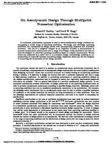
Optimized

Baseline

Optimized

Baseline

ANNAPOLIS, MD

2

Contents 1

2

Introduction ................................................................................................................................ 10

1.2 1.3 1.4

Complexity of Flow ............................................................................................................................................. 10 Computational Cost ............................................................................................................................................ 10 Aerodynamic Optimization ............................................................................................................................. 12

Airplane Design ......................................................................................................................... 13 2.1

Role of CFD in the Design Process ................................................................................................................ 13 Conceptual Design .................................................................................................................................. 13 Preliminary Design................................................................................................................................. 13 Detailed or Final Design ....................................................................................................................... 13 2.2 Conceptual Aerodynamic Design Process as Applied to Airplanes ............................................... 13 Purpose and Scope of Conceptual Airplane Design .................................................................. 13 Cost Estimation ........................................................................................................................................ 14 Preliminary Weight Estimation ........................................................................................................ 14 Breguet Range Estimation................................................................................................................... 14 Aerodynamic Considerations............................................................................................................. 15 Wing Design and Selection of Wing Parameters ........................................................................ 15 Wing Selection (Airfoils) .......................................................................................... 16 Presentation of Aerodynamic Characteristics of Airfoils ........................................ 16 Geometrical Characteristics of Airfoils .................................................................... 16 Airfoil Shape and Ordinates..................................................................................... 16 Airfoil Nomenclature ............................................................................................... 18 NACA Four-Digit Series Airfoils ................................................................................ 18 NACA Five-Digit Series Airfoils ................................................................................. 18 Six Series Airfoils...................................................................................................... 19 NASA Airfoils ............................................................................................................ 19 Estimation of Wing Loading & Thrust Loading .......................................................................... 19 Structural Considerations ................................................................................................................... 20 Environmental Impacts ........................................................................................................................ 20 Airplane Noise ......................................................................................................... 21 Emissions ................................................................................................................. 21 Performance Estimation ...................................................................................................................... 21 General Remarks on Performance Estimation ........................................................ 22 Fuselage and Tail Sizing ........................................................................................... 23 Tail cone/Rear Fuselage: ......................................................................................... 23 Estimation of Wing and Thrust Loading Based on Conception Design ............................ 24 Remarks on for choosing Wing Loading and Thrust Loading or Power Loading ..... 24 Selection of Wing Loading based on Landing Distance ........................................... 25 Wing Loading from Landing Consideration based on Take-off Weight .................. 25 Stability and Controllability................................................................................................................ 25 Static Longitudinal Stability and Control ................................................................. 25 2.3 Aerodynamic Design and Analysis Coupling for Wing ........................................................................ 26 The Straight Wing Configuration...................................................................................................... 26 The Swept Wing Configuration ......................................................................................................... 27 2.3.2 The Rear Fuselage Mounted Engine Configuration .................................................................. 28 2.4 Control Theory Approach to Transport Airplane Design ................................................................... 29

3

2.5 2.6

3

Aerodynamic Optimization Problem ................................................................................. 34 3.1 3.2

3.3 3.4

3.5 3.6

3.7

3.8

4

Design of Wing Planform ..................................................................................................................... 29 Thought on Hierarchal Design Approach .................................................................................................. 31 Classification of Design Optimization Methods ...................................................................................... 32 Direct Design............................................................................................................................................. 32 Inverse Design .......................................................................................................................................... 32

Role of Optimization .......................................................................................................................................... 34 Types of Optimization & Searches ............................................................................................................... 35 Continuous Vs. Discrete Optimization ........................................................................................... 35 Unconstrained Vs. Constrained Optimization ............................................................................. 35 Deterministic Vs. Stochastic Optimization ................................................................................... 35 Quantity of Objectives Functions ..................................................................................................... 35 Single Vs. Multi-Objective Optimization ................................................................. 36 Various Methods to Solve Multiple Objective Optimization................................... 37 Pareto Optimality .................................................................................................... 38 Gradient-Based Optimization Methods...................................................................................................... 38 Traditional Gradient-Based Method (GBM)................................................................................. 39 Adjoint Variable Method (AV) ........................................................................................................... 39 Stochastic Optimization Method ................................................................................................................... 40 Design of Experiment (DOE) .............................................................................................................. 40 Surrogate Model (SM) ........................................................................................................................... 41 Simulated Annealing (SA) ................................................................................................................... 41 Genetic Algorithms (GA) ...................................................................................................................... 42 Evolutionary Algorithms (EAs) ......................................................................................................... 42 Data Mining ............................................................................................................................................... 42 Aerodynamic Shape Optimization ............................................................................................................... 43 Statement of Optimization Problem ............................................................................................................ 44 Multi-Objective vs. Multi-Level Optimization ............................................................................. 45 Multi-Point Optimization Over a Fight Envelope ...................................................................... 45 Case Study – Multi-Point Optimization of Airfoil ....................................................................... 46 Geometric Representation .............................................................................................................................. 47 Discrete Approach .................................................................................................................................. 48 Analytical Approach............................................................................................................................... 49 Partial Differential Equation Approach ......................................................................................... 49 Spline Based Parameterization ......................................................................................................... 50 Free-Form Deformation Approach (FFD) ................................................................ 51 Class/Shape Function Transformation Method (CST) ............................................................ 52 CST Airfoils & Wings ................................................................................................ 53 Case Study - Airfoil Optimization............................................................................. 53 Constraint Handling ........................................................................................................................................... 55

Gradient-Based Methods for Aerodynamic Optimizations ........................................ 57

4.1 4.2 4.3 4.4 4.5

Sensitivity Analysis............................................................................................................................................. 58 Aero-Elastic Optimization .............................................................................................................................. 59 Multi-Point Optimization ................................................................................................................................. 60 Acceleration Technique for Multi-Level Optimization ....................................................................... 61 Effect of Variable Cant Angle Winglet in Aircraft Control .................................................................. 61 Comparison of Cant Angle Winglet for Simulation vs. Wind Tunnel ................................. 62

4

4.6 The C-Wing Layout ............................................................................................................................................. 63 4.7 Case Study 1 - Comparison of Point Design and Range-Based Objectives for Transonic Airfoil Optimization ........................................................................................................................................................ 64 Statement of Problem ........................................................................................................................... 64 Discussion and Literature Survey .................................................................................................... 64 Flow Solver and Meshes....................................................................................................................... 67 Generic Single-Objective Optimization .......................................................................................... 68 Range Optimization with Varying Design Point ......................................................................... 69 Analytical Treatment for Fixed Shape ............................................................................................ 71 Expression for Optimal Mach .................................................................................. 71 Results ..................................................................................................................... 72 Numerical Correlation ............................................................................................. 73 Inviscid Range Optimizations ............................................................................................................ 74 Comparison of Approaches for Viscous Optimization ............................................................. 76 Single-Point and Multi-Point Optimization ............................................................. 76 Range Optimization ................................................................................................. 77 Off-Design Performance ....................................................................................................................... 80 Concluding Remarks .............................................................................................................................. 81 4.8 Case Study 2 - Wing Aerodynamic Optimization using Efficient MathematicallyExtracted Modal Design Variables ............................................................................................................................ 81 Statement of Problem ........................................................................................................................... 81 Introduction and Background ........................................................................................................... 82 Shape Parameterization & Literature Review ............................................................................ 83 Other Parameterization Techniques ....................................................................... 85 Shape Optimization using Multi-Resolution Subdivision Curves ............................ 86 Shape Deformations by Singular Value Decomposition (SVD) ............................................ 87 RBF Coupling of Point Sets for Airfoil Deformation ................................................................. 89 Control Point Deformations ............................................................................................................... 90 Computation of Deformation Field in 2D ...................................................................................... 91 Computation of Deformation Field in 3D ...................................................................................... 92 Optimization Approach ........................................................................................................................ 94 Feasible Sequential Quadratic Programming (FSQP) .............................................. 95 Flow Solver ................................................................................................................................................ 96 Application of Modal Design Variables in 3D .............................................................................. 96 Problem Definition .................................................................................................. 96 Results.................................................................................................................... 98 Conclusions ............................................................................................................................................ 100 4.9 Case Study 3 - Gradient Based Aerodynamic Shape Optimization Applied to a Common Research Wing (CRM) ............................................................................................................................. 100 Methodology .......................................................................................................................................... 101 Geometric Parametrization ................................................................................... 102 Mesh Perturbation ................................................................................................ 102 CFD Solver.............................................................................................................. 103 Optimization Algorithm ......................................................................................... 103 Problem Formulation ......................................................................................................................... 103 Mesh Convergence Study ...................................................................................... 104 Optimization Problem Formulation ...................................................................... 105 Single-Point Aerodynamic Shape Optimization ...................................................................... 105 Effect of the Number of Shape Design Variable....................................................................... 106

5

Acceleration Technique for Multi-Level Optimization ........................................................ 107 Multi-Point Aerodynamic Shape Optimization ........................................................................ 108 Strength of Multi-Point Optimization .......................................................................................... 109

5

Non-Gradient Methods for Aerodynamic Optimizations ......................................... 111 Genetic Algorithms (GA) ................................................................................................................... 111 Framework for the Shape Optimization of Aerodynamic using Genetic Algorithms (GA) ......................................................................................................................... 112 Application of Hybrid Algorithms to Aerodynamic Optimizations ................................. 113 Application of Surrogate Modelling to Aerodynamic Optimization................................ 115 Artificial Neutral Networks (ANN) ......................................................................... 117 Kriging Model ........................................................................................................................................ 118 Gradient-Enhanced Kriging.................................................................................... 119

6

7

Sensitivity Analysis and Aerodynamic Optimization ................................................ 121

6.1 6.2 6.3 6.4 6.5

Aerodynamic Sensitivity ............................................................................................................................... 122 Flow Analysis and Sensitivity Equation .................................................................................................. 123 Optimization....................................................................................................................................................... 124 Surface Modeling Using NURBS ................................................................................................................. 125 Case Study - 2D Study of Airfoil Grid Sensitivity via Direct Differentiation (DD) ................. 127 2D Case Study- Airfoil Grid, Flow Sensitivity, and Optimization .................................... 128 Discussions ............................................................................................................................................. 129 6.6 Extension to 3D using Automatic Differentiation (AD) .................................................................... 130 6.7 Essence of Adjoint Equation ........................................................................................................................ 131 The Adjoint Reverses the Propagation of Information ........................................................ 131 The Adjoint Equation is Linear....................................................................................................... 132 6.8 Classical Formulation of the Adjoint Variable (AV) Approach to Optimal Design ................ 132 Limitations of the Adjoint Approach............................................................................................ 135 Constraints ............................................................................................................ 135 Limitations of Gradient-Based Optimization ......................................................... 135 Case Study – Adjoint Aero-Design Optimization for Multi-Stage Turbomachinery Blades ...................................................................................................................................... 136

Turbo-Machinery Design and Optimization ................................................................. 138

7.1 7.2 7.3

A Road Map to Turbo-Machine Design and Optimization ............................................................... 138 Optimization Methods for Turbomachinery Designs........................................................................ 139 Wu’s Pioneering (S1 and S2) Scheme .......................................................................................... 141 Concept of Streamline Curvature Method ................................................................................. 141 Case Study 1 - Aerodynamic Design of Compressors ........................................................................ 142 Statement of Problem ........................................................................................................................ 142 Different Compressors Objectives ................................................................................................ 143 Design Techniques for Compressor ............................................................................................. 144 Preliminary Design Techniques (1D) .......................................................................................... 146 Through Flow Design Techniques (2D) ...................................................................................... 146 Detailed Design Techniques (3D) ................................................................................................. 148 Direct Methods ...................................................................................................... 148 Inverse Methods.................................................................................................... 148 Concluding Remarks ........................................................................................................................... 149

6

7.4

Case Study 2 – Turbine Airfoil Optimization using Quasi 3D Analysis Codes ......................... 150 Parametric Representation of Airfoil Design Process .......................................................... 151 Constraints and Problem Formulation ....................................................................................... 152 Quasi-3D CFD Analysis and Results ............................................................................................. 154 Concluding Remarks ........................................................................................................................... 156 7.5 Case Study 3 – 2D Design Optimization of Turbine Blade in Quasi-Periodic Unsteady Flow Problems Using a Harmonic Balance Method ....................................................................................... 157 OptC1Configuration ............................................................................................................................ 158 Optimization Problem and Results ............................................................................................... 158

8

Multi-Disciplinary Optimization (MDO) ........................................................................ 162

8.1 8.2 8.3 8.4 8.5 8.6

8.7

Background......................................................................................................................................................... 162 Computational Cost Associated with MDO ............................................................................................ 162 Organizational Complexity ........................................................................................................................... 163 Clarification of Some Terminology ........................................................................................................... 163 Categories of MDO Analysis ......................................................................................................................... 163 MDO Components ............................................................................................................................................ 164 MDO Components as Environed by [Sobieszczanski-Sobieski]........................................ 164 Mathematical Modeling of a System .................................................................... 164 Trade Off between Accuracy and Cost in MDO..................................................... 165 Design-Oriented Analysis ...................................................................................... 165 Approximation Concepts Applicable to MDO ....................................................... 166 System Sensitivity Analysis .................................................................................... 167 Optimization Procedures with Approximations and Decompositions .................. 168 Human Factor ........................................................................................................ 169 MDO Formulation as Depicted by Wikipedia ........................................................................... 170 Design Variables .................................................................................................... 170 Constraints ............................................................................................................ 170 Objective................................................................................................................ 170 Models ................................................................................................................... 171 Simple Optimization .............................................................................................. 171 Problem Solution ................................................................................................... 171 Approaches to MDO for Turbomachinery Engine Applications ................................................... 171 Overall Design Process ...................................................................................................................... 172 Single Discipline Optimization ....................................................................................................... 173 Aerodynamic Design Optimization for Turbomachinery .................................................... 173 Axial Compressor Gas path Optimization.............................................................. 174 Turbine Gas path Optimization ............................................................................. 175 Concluding Remarks ........................................................................................................................... 175

List of Tables: Table 3.1 Performance Comparison of Initial an Optimize Airfoils (Courtesy of 44) ....................... 54 Table 4.1 Analytical optimal Breguet Mach Numbers as a Fraction of Mc for NACA 0012 using M2CL as a .................................................................................................................................................................. 73 Table 4.2 Results for Inviscid Range Optimizations ..................................................................................... 74 Table 4.3 Results for Inviscid Range Optimizations with k = 0.04 Induced Drag Factor .............. 75 Table 4.4 Results for Drag Minimizations ......................................................................................................... 77 Table 4.5 Results for Viscous Range Optimizations with k = 0:04 and 0.1 ........................................ 78

7

Table 4.6 Optimization Results (CD in Counts) .............................................................................................. 98 Table 4.8 Aerodynamic Shape Optimization Problem - (Courtesy of Martins and Hwang) ...... 104 Table 4.7 Mesh Convergence Study for the Baseline CRM Wing - (Courtesy of Martins and Hwang).............................................................................................................................................................................. 104 Table 6.1 Aerodynamic Sensitivity Coefficient ............................................................................................ 129 Table 6.2 Design improvement for an Airfoil ............................................................................................... 130 Table 7.1 Axial Flow Compressor Design ....................................................................................................... 143 Table 7.2 Airfoil Geometry Parameters .......................................................................................................... 153 Table 7.3 Airfoil Design Variables ..................................................................................................................... 154

List of Figures: Figure 1.1 Hierarchy of Models for Industrial Applications ...................................................................... 10 Figure 1.2 Cp Contours on High Lift Configuration with 22 M cells model ......................................... 11 Figure 2.1 Aerodynamic Characteristics of an Airfoil .................................................................................. 17 Figure 2.2 Rear fuselage shape .............................................................................................................................. 23 Figure 2.3 Pressure Distribution for wing-pylon-nacelle Configuration; (Initial left), (refined right) ................................................................................................................................................................... 26 Figure 2.4 Over Wing Mounted Engines Configuration............................................................................... 27 Figure 2.5 Under Wing Mounted Engines Configuration ............................................................................ 27 Figure 2.6 Rear Fuselage Mounted Engines Configuration........................................................................ 28 Figure 2.7 Leading Edge Droop and Vortilons ................................................................................................ 28 Figure 2.8 Simplified Wing Planform of a ......................................................................................................... 30 Figure 2.9 Redesigned Boeing 747 Wing at Mach 0.86 based on Cp Distributions ........................ 30 Figure 2.10 Tightly Coupled Two Level Design Process ............................................................................. 31 Figure 3.1 Global Maximum of f (x, y) ................................................................................................................. 34 Figure 3.2 Different Search and Optimization Techniques ........................................................................ 37 Figure 3.3 Pareto Optimal....................................................................................................................................... 38 Figure 3.4 Comparison of the Full Factorial and Latin Hypercube data points (Courtesy of [Li & Zheng]) ...................................................................................................................................................................... 40 Figure 3.5 Multi-Point Design Process as Envisioned by Jameson – (Courtesy of Jameson et al.) 46 Figure 3.6 Wing configurations at different flight phases (Courtesy of Chiguluri).......................... 47 Figure 3.7 NURBS Surfaces Parametrizing Surface Blend on Fuselage (Courtesy of Vecchia & Nicolosi) .......................................................................................................................................................................... 51 Figure 3.8 Free-Form Deformation (FFD) Parametrizing Wing with 720 Control Points (Courtesy of Kenway and Martins) .......................................................................................................................... 52 Figure 3.9 Contours of the Initial Airfoil (Left) an Optimize Airfoil (Right)44 .................................... 54 Figure 3.10 Concept of using Parallel Evaluation Strategy of Feasible and Infeasible Solutions to Guide Optimization Direction in a GA............................................................................................ 56 Figure 4.1 Gradient-Based Aerodynamic Optimization Process ............................................................. 57 Figure 4.2 High Performance Low Drag for Single and Multiple Design Points (Courtesy of [Kenway & Martins])...................................................................................................................................................... 60 Figure 4.3 Un-Symmetric Wing-Tip Arrangement for a Sweptback Wing to Initiate ..................... 61 Figure 4.4 Lift-to-Drag Ratio, L/D (Wind Tunnel and CFD Comparison)............................................. 62 Figure 4.5 C-Wing Layout with Positive Direction of Span-Loading on Each Surface Indicated.............................................................................................................................................................................. 63 Figure 4.6 Range variation with Mach number for Boeing 747 (where l is the nondimensional wing loading) .......................................................................................................................................... 66 Figure 4.7 Airfoil Meshing ....................................................................................................................................... 67

8

Figure 4.8 Comparison of Constraint Influence on Mopt for NACA 0012 .............................................. 72 Figure 4.9 Mach Sweeps at Fixed l showing ML/D ........................................................................................ 73 Figure 4.10 Surface Shapes and CP for Inviscid Range Optimizations of NACA0012 at Different Lift Values with Induced Drag Penalty ................................................................................................ 76 Figure 4.11 Surface Shapes & Cp for Viscous Range Optimizations ....................................................... 79 Figure 4.12 Surface Shapes for Drag Minimizations ..................................................................................... 79 Figure 4.13 Drag Curve at Design CL of Optimized Airfoils ........................................................................ 80 Figure 4.14 M-CL maps with normalized ML/D Contours of Optimized airfoils (97% contour highlighted) ...................................................................................................................................................... 80 Figure 4.15 Volume of solid (VOS) design variables as grey-scale and RSVS profile in red; 1 corresponds to a completely full cell and 0 an empty cell. ......................................................................... 85 Figure 4.16 Four Levels of Subdivision of a Four Point Control Polygon ............................................ 86 Figure 4.17 Generic Non-Symmetric Airfoil Modes - a Mode 1. b Mode 2. c Mode 3. d Mode 4. e Mode 5.......................................................................................................................................................................... 88 Figure 4.18 Surface-Based Control Points and Example Deformation. a Control Points. b Example Deformation .................................................................................................................................................... 91 Figure 4.19 Surface Mesh and Control Points in 3D ..................................................................................... 92 Figure 4.21 Surface and Control Point Modal Deformations. a Mode 1 global. b Mode 3 global. c Mode 5 ................................................................................................................................................................ 93 Figure 4.20 Surface Mesh and off-Surface Control Points .......................................................................... 94 Figure 4.22 Domain and Block Boundaries and far-field Mesh................................................................ 98 Figure 4.23 Upper Surface Pressure Coefficient. a Initial Geometry. b Domain Element. c 10 Global Modes ,d 10 Local Modes ......................................................................................................................... 99 Figure 4.24 Convergence Histories ................................................................................................................... 100 Figure 4.25 Shape Design Variables are the z-Displacements of 720 FFD Control Points (Courtesy of Martins and Hwang) ......................................................................................................................... 102 Figure 4.26 Optimized Wing with Shock-Free with 8.5% Lower Drag – (Courtesy of Lyu and Martins) ................................................................................................................................................................... 105 Figure 4.27 Insensitivity of Number of Optimization Iterations to Number of Design Parameters ...................................................................................................................................................................... 107 Figure 4.28 Multipoint Optimization Flight Conditions ........................................................................... 108 Figure 4.29 Multi-Point Optimized - (Courtesy of Lyu and Martins) .................................................. 109 Figure 4.30 Comparison of Baseline, Single, and Multipoint Optimization...................................... 109 Figure 5.1 Sketch of Griewank Function on larger scale (left) Vs. smaller scale (right) ............. 111 Figure 5.2 Optimization Scheme (GA) ............................................................................................................. 113 Figure 5.3 Hybrid Organic-Optimization Algorithm .................................................................................. 115 Figure 5.4 Artificial Neural Network (ANN) Configuration .................................................................... 117 Figure 5.5 Artificial Neural Networks (ANN) with 1 & 2 Hidden Layers .......................................... 118 Figure 5.6 Prediction Comparison of the Rosenbrock function based on Kriging Model and GEK Model............................................................................................................................................................... 119 Figure 6.1 Methods of Evaluating Sensitivity Derivatives....................................................................... 123 Figure 6.2 Optimization Strategy Loop ........................................................................................................... 125 Figure 6.3 B-Spline approximation of NACA0012 (left) and RAE2822 (right) airfoils ............... 126 Figure 6.4 Sample grid and grid sensitivity................................................................................................... 127 Figure 6.5 Free form deformation (FFD) volume with control points (Courtesy of Kenway et al.) 128 Figure 6.6 Optimization Cycle History............................................................................................................. 128 Figure 6.7 Original and Optimized Airfoil ...................................................................................................... 129 Figure 6.8 3D Volume grid and sensitivty w.r.t. wing root chord ........................................................ 130 Figure 6.9 Propagation of Information............................................................................................................ 132

9

Figure 6.10 Aerodynamic Shape Optimization Procedure using Adjoint Variable as Sensitivity Analysis ...................................................................................................................................................... 134 Figure 6.11 Pressure Contours ........................................................................................................................... 136 Figure 7.1 General Description of Computational Planes........................................................................ 138 Figure 7.2 Turbomachine Design Process...................................................................................................... 139 Figure 7.3 Optimization Process for Turbomachinery ............................................................................. 140 Figure 7.4 Sketch of a Compressor Stage (left) and Cascade of Geometries at Mid- Span (right) ................................................................................................................................................................................ 144 Figure 7.5 Compressor design flow chart ...................................................................................................... 145 Figure 7.6 Preliminary Estimation of Number of Stages in Compressor .......................................... 146 Figure 7.7 Optimization Procedures proposed in [Massardo et al.] ................................................... 147 Figure 7.8 Comparison of Blade Loading Prescribed by Inverse Mode ............................................. 149 Figure 7.9 The turbine design process ............................................................................................................ 150 Figure 7.10 Parametric Representation of an Airfoil ............................................................................... 152 Figure 7.11 Sample Mach Number Distribution .......................................................................................... 152 Figure 7.12 Flow path of the turbine ............................................................................................................... 155 Figure 7.13 Schematics of an airfoil showing stream lines along the radial direction ................ 155 Figure 7.14 3D model of an airfoil showing the passage between adjacent airfoils .................... 156 Figure 7.15 Schematic Geometry of theT106D-IZ Turbine Cascade ................................................... 157 Figure 7.16 Total Pressure Loss Coefficient Evolution in time Calculated with URANS Simulation for both the Baseline and the Optimized Configuration ....................................................... 159 Figure 7.17 Shape Optimization History of the Total Pressure Loss Coefficient and Comparison Between Baseline and Optimized Blade Profile (OptC1) ................................................... 159 Figure 7.18 Mach Number Contours calculated at Three Different Time Instances with the HB Method, Based on theOptC1 test case, for both the Baseline (a), (b), (c) and the Optimized (d), (e), (f) Blade Profile ...................................................................................................................... 160 Figure 0.1 Product, components and the supporting disciplines ......................................................... 172 Figure 0.2 Aerodynamic design process for Turbomachinery .............................................................. 173 Figure 0.3 Comparison of "Baseline" and "Optimized" Turbine Mean Line Results .................... 175

10

1 Introduction 1.2 Complexity of Flow The complexity of fluid flow is well illustrated in Van Dyke’s Album of Fluid Motion. Many critical phenomena of fluid flow, such as shock waves and turbulence, are essentially nonlinear and the disparity of scales can be extreme. The flows of interest for industrial applications are almost invariantly turbulent. The length scale of the smallest persisting eddies in a turbulent flow can be estimated as of order of 1/Re3/4 in comparison with the macroscopic length scale. In order to resolve such scales in all three spatial dimensions, a computational grid with the order of Re9/4 cells would be required. Considering that Reynolds numbers of interest for airplanes are in the range of 10 to 100 million, while for submarines they are in the range of , the number of cells can easily overwhelm any foreseeable supercomputer. [Moin and Kim] reported that for an airplane with 50-meter-long fuselage and wings with a chord length of 5 meters, cruising at 250 m/s at an altitude of 10,000 meters, about 10 quadrillions (1016) grid points are required to simulate the turbulence near the surface with reasonable details. They estimate that even with a sustained performance of 1 Teraflops, it would take several thousand years to RANS (1990s) simulate each second of flight time. Spalart has estimated that if computer performance continues to increase at the present rate, the Direct Numerical Euler (1980s) Simulation (DNS) for an aircraft will be feasible in 2075. Non-linear Consequently mathematical models Potential (1970s) with varying degrees of simplification have to be introduced in order to make Linear Potential computational simulation of flow (1960s) feasible and produce viable and costeffective methods. Figure 1.1 indicates a hierarchy of models at different levels of simplification which Figure 1.1 Hierarchy of Models for Industrial Applications have proved useful in practice. Inviscid calculations with boundary layer corrections can provide quite accurate predictions of lift and drag when the flow remains attached. The current main CFD tool of the Boeing Commercial Airplane Company is TRANAIR, which uses the transonic potential flow equation to model the flow. Procedures for solving the full viscous equations are needed for the simulation of complex separated flows, which may occur at high angles of attack or with bluff bodies. In current industrial practice these are modeled by the Reynolds Average Navier Stokes (RANS) equations with various turbulence models1.

1.3 Computational Cost In external aerodynamics most of the flows to be simulated are steady, at least at the macroscopic scale. Computational costs vary drastically with the choice of mathematical model. Studies of the dependency of the result on mesh refinement, performed by this author and others, have demonstrated that inviscid transonic potential flow or Euler solutions for an airfoil can be accurately Antony Jameson and Massimiliano Fatica, “Using Computational Fluid Dynamics for Aerodynamics”, Stanford University, USA. 1

11

calculated on a mesh with 160 cells around the section, and 32 cells normal to the section. Using a new non-linear Symmetric Gauss-Siedel (SGS) algorithm, which has demonstrated “text book” multigrid convergence (in 5 cycles), two-dimensional calculations of this kind can be completed in 0.5 seconds on a laptop computer (with a 2Ghz processor). A three dimensional simulation of the transonic flow over a swept wing on a 192 x 32 x 32 mesh (196,608 cells) takes 18 seconds on the same laptop. Moreover it is possible to carry out an automatic redesign of an airfoil to minimize its shock drag in 6.25 seconds, and to redesign the wing of a Boeing 747 in 330 seconds2. Viscous simulations at high Reynolds numbers require vastly greater resources. On the order of 32 mesh intervals are needed to resolve a turbulent boundary layer, in addition to 32 intervals between the boundary layer and the far field, leading to a total of 64 intervals. In order to prevent degradations in accuracy and convergence due to excessively large aspect ratios (in excess of 1,000) in the surface mesh cells, the chord wise resolution must also be increased to 512 intervals. Translated to three dimensions, this implies the need for meshes with 5-10 million cells (for example, 512 x 64 x 256 = 8,388,608 cells) for an adequate simulation of the flow past an isolated wing. When simulations are performed on less fine meshes with, say, 0.5 M to 1 M cells, it is very hard to avoid mesh dependency in the solutions as well as sensitivity to the turbulence model. Currently Boeing uses meshes with 15-60 million cells for viscous simulations of commercial aircraft with their high lift systems deployed3. Figure 1.2 show the Cp contours on High Lift Configuration (wing) with 22 M Cells (Courtesy of Boeing). Using a multigrid algorithm, 2000 or more cycles are required to reach a steady state, and it takes 1-3 days to turn around the calculations on a 200 processor Beowulf cluster.

Figure 1.2

Cp Contours on High Lift Configuration with 22 M cells model

Antony Jameson and Massimiliano Fatica, “Using Computational Fluid Dynamics for Aerodynamics”, Stanford University. 3 Boing using 22 M Cells on High lift Configuration. 2

12

1.4 Aerodynamic Optimization The use of computational simulation to scan many alternative designs has proved extremely valuable in practice, but it is also evident that the number of possible design variations is too large to permit their complete evaluation. Thus it is very unlikely that a truly optimum solution can be found without the assistance of automatic optimization procedures. To ensure the realization of the true best design, the ultimate goal of computational simulation methods should not just be the analysis of prescribed shapes but the automatic determination of the true optimum shape for the intended application. The need to find optimum aerodynamic designs was already well recognized by the pioneers of classical aerodynamic theory. A notable example is the determination that the optimum span-load distribution that minimizes the induced drag of a monoplane wing is elliptic [Glauert]4, [Prandtl and Tietjens]5. There are also a number of famous results for linearized supersonic flow. The body of revolution of minimum drag was determined by Sears6, while conditions for minimum drag of thin wings due to thickness and sweep were derived by Jones7. The problem of designing a two-dimensional profile to attain a desired pressure distribution was studied by [Lighthill]8, who solved it for the case of incompressible flow with a conformal mapping of the profile to a unit circle. As an vital “ingredients” in Gradient Base Optimization, the sensitivities may now be estimated by making a small variation in each design parameter in turn and recalculating the flow. The gradient can be determined directly or indirectly by number of available methods, including Direct Differentiation (DD), Adjoin Variable(AV), Symbolic Differentiation (SD), Automatic Differentiation (AD), and Finite Difference (FD). Once the gradient has been calculated, a descent method can be used to determine a shape change that will make an improvement in the design. The gradients can then be recalculated, and the whole process can be repeated until the design converges to an optimum solution, usually within 50–100 cycles. The fast calculation of the gradients makes optimization computationally feasible even for designs in three-dimensional viscous flow. However, there is a possibility that the descent method could converge to a local minimum rather than the global optimum solution.

Glauert, H. (1926), “The Elements of Aero foil and Airscrew Theory”, Cambridge University Press. Prandtl, L. and Tietjens, O.G. (1934), “Applied Hydro and Aerodynamics”, Dover Publications. 6 Sears, W.D. (1947), ”On projectiles of minimum drag”, Q. Appl. Math., 4, 361–366. 7 Jones, R.T. (1981), ”The minimum drag of thin wings in frictionless flow”. J. Aerosol Sci., 18, 75–81. 8 Lighthill, M.J. (1945), ”A new method of two dimensional aerodynamic design”. Rep. Memor. Aero. Res. Coun. Lond., 2112, 143–236. 4 5

13

2 Airplane Design 2.1 Role of CFD in the Design Process

The actual use of CFD by Aerospace companies is a consequence of the trade-off between perceived benefits and costs. While the benefits are widely recognized, computational costs cannot be allowed to swamp the design process9. The need for rapid turnaround, including the setup time, is also crucial. In current industrial practice, the design process can generally be divided into three phases: 1. Conceptual Design, 2. Preliminary Design, 3. Detailed Design. Conceptual Design The conceptual design stage, typically carried out by a staff of 15 - 30 engineers, defines the mission in the light of anticipated market requirements, and determines a general preliminary configuration, together with first estimates of size, weight and performance. The costs of this phase, depending on application (i.e., airplane configuration), and costs in the range of $M 6-12. Preliminary Design In the preliminary design stage the aerodynamic shape and structural skeleton progress to the point where detailed performance estimates can be made and guaranteed to potential customers, who can then, in turn, formally sign binding contracts for the purchase of a certain number of aircraft. A staff of 100-300 engineers is generally employed for up to 2 years, at a cost of $M60 - 120 (again the same application). Initial aerodynamic performance is explored by computational simulations and through wind tunnel tests. While the costs are still fairly moderate, decisions made at this stage essentially determine both the final performance and the development costs. Detailed or Final Design In the final design stage the structure must be defined in complete detail, together with complete systems, including the flight deck, control systems (involving major software development for flyby-wire systems), avionics, electrical and hydraulic systems, landing gear, weapon systems for military aircraft, and cabin layout for commercial aircraft. Major costs are incurred at this stage, during which it is also necessary to prepare a detailed manufacturing plan. Thousands of engineers define every part of the aircraft. Total costs are $B 3-10. Therefore, the final design would normally be carried out only if sufficient orders have been received to indicate a reasonably high probability of recovering a significant fraction of the investment10.

2.2 Conceptual Aerodynamic Design Process as Applied to Airplanes In the development of commercial aircraft, aerodynamic design plays a leading role during the conceptual and preliminary design stage, Ultimately, the definition of the external aerodynamic shape is typically finalized after a detailed analysis. Purpose and Scope of Conceptual Airplane Design The process of design of a device or a vehicle, in general involves the use of knowledge in diverse fields to arrive at a product that will satisfy requirements regarding functional aspects, operational safety and cost. The design of an airplane, which is being dealt in this course, involves synthesizing knowledge in areas like aerodynamics, structures, propulsion, systems and manufacturing Antony Jameson and, assisted by, Kui Ou, “Optimization Methods in Computational Fluid Dynamics”, Aeronautics and Astronautics Department, Stanford University, Stanford, CA, USA. 10 See Previous. 9

14

techniques. The aim is to arrive at the configuration of an airplane, which will satisfy abovementioned requirements. The design of an airplane is a complex engineering task. which generally involves the following among others:            

Obtaining the specifications of the airplane, selecting the type and determining; Aerodynamic Considerations; Wing design; Optimization of wing loading and thrust loading; Fuselage design, preliminary design of tail surface and preliminary layout; Center of Gravity calculation; the geometric parameters for different surfaces; Preliminary weight estimation; Estimates of areas for horizontal and vertical tails; Engine Selection; Detail Structural design; Determination of airplane performance, stability, and structural integrity from flight tests.

The aerodynamic lines of the Boeing 777 were frozen, for example, when initial orders were accepted, before the initiation of the detailed design of the structure. The starting point is an initial CAD definition resulting from the conceptual design. The inner loop of aerodynamic analysis is contained in an outer multi-disciplinary loop, which is in turn contained in a major design cycle involving wind tunnel testing. In recent Boeing practice, three major design cycles, each requiring about 4-6 months, have been used to finalize the wing design. Improvements in CFD, might allow the elimination of a major cycle, would significantly shorten the overall design process and reduce costs. Moreover, the improvements in the performance of the final design, which might be realized through the systematic use of CFD, could have a crucial impact. Cost Estimation An improvement of 5 percent in lift to drag (L/D) ratio directly translates to a similar reduction in fuel consumption. With the annual fuel costs of a long-range airliner in the range of $5-10 million, a 5 percent saving would amount to a saving of the order of $10 million over a 25 year operational life, or $5 billion for a fleet of 500 aircraft. In fact an improvement in L/D enables a smaller aircraft to perform the same mission, so that the actual reduction in both initial and operating costs may be several times larger. Furthermore a small performance advantage can lead to a significant shift in the share of a market estimated to be more than $1 trillion over the next decades. Preliminary Weight Estimation An accurate estimate of the weight of the airplane is required for the design of the airplane. This is arrived at in various stages. In the last chapter, the procedure to obtain the first estimate of the gross weight was indicated. This was based on the ratio of the payload to the gross weight of similar airplanes. This estimate of the gross weight is refined by estimating (a) the fuel fraction i.e. weight of fuel required for the proposed mission of the airplane, divided by gross weight and (b) empty weight fraction i.e. empty weight of airplane divided the gross weight. Breguet Range Estimation A good first estimate of performance is provided by the Breguet range equation:

Range 

W  Wf VL 1 log 0 D SFC W0

Eq. 2.1

15

Here V is the speed, L/D is the lift to drag ratio, SFC is the specific fuel consumption of the engines, W0 is the loading weight (empty weight + payload + fuel resourced), and Wf is the weight of fuel burnt. Eq. 2.1 displays the multidisciplinary nature of design. A light structure is needed to reduce W 0. SFC is the province of the engine manufacturers. The aerodynamic designer should try to maximize VL/D. This means the cruising speed V should be increased until the onset of drag rise at a Mach Number M = V/C ∼ 0.85. But the designer must also consider the impact of shape modifications in structure weight11. An excellent discussion of these and other factors in design of airplane, is documented by [Tulapurkara]12 and readers encourage to consult the on-line material. Aerodynamic Considerations A poorly designed external shape of the airplane could result in undesirable flow separation resulting in low CLmax, low lift to drag ratio and, large transonic and supersonic wave drag. Following remarks can be deducted:  Minimization of wetted area is an important consideration as it directly affects skin friction drag and in turn parasite drag. One way to achieve this is to have smallest fuselage diameter and low excellence ratio (between 3 and 4). However, proper space for payload, ease of maintenance and tail arm also needs to be considered.  To prevent flow separation, the deviation of fuselage shape from free stream direction should not exceed 10 – 12 degrees .  Proper fillets should be used at junctions between  wing and fuselage,  fuselage and tails and  wing and pylons.  Base area should be minimum.  Canard, if used, should be located such that its wake does not enter the engine inlet as it may cause engine stalling.  Area ruling The plan view of supersonic airplanes indicates that the area of cross section of fuselage is decreased in the region where wing is located. This is called area ruling. A brief note on this topic is presented below. It was observed that the transonic wave drag of an airplane is reduced when the distribution of the area of cross section of the airplane, in planes perpendicular to the flow direction, has a smooth variation. In this context, it may be added that the area of cross section of the fuselage generally varies smoothly. However, when the wing is encountered there is an abrupt change in the cross sectional area. This abrupt change is alleviated by reduction in the area of cross section of fuselage in the region where the wing is located. Such a fuselage shape is called ‘Coke-bottle shape’. Wing Design and Selection of Wing Parameters In the context of wing design the following aspects need consideration:  Wing area (S) : This is calculated from the wing loading and gross weight which have been already decided i.e. S = W/(W/S)  Location of the wing on fuselage : High-, low- or mid-wing  Airfoil : Thickness ratio, camber and shape Antony Jameson, “Airplane Design with Aerodynamic Shape Optimization”, Aeronautics & Astronautics Department, Stanford University, 2010. 12 E.G. Tulapurkara, ”Airplane design(Aerodynamic)”, Dept. of Aerospace Engineering., Indian Institute of Technology, Madras, India. 11

16

 Sweep : Whether swept forward, swept backward, angle of sweep, cranked wing, variable sweep.  Aspect ratio : High or low, winglets  Taper ratio : Straight taper or variable taper.  Twist: Amount and distribution  Wing incidence or setting  High lift devices : Type of flaps and slats; values of CLmax, Sflap/S  Ailerons and spoilers : Values of Saileron/S; Sspoiler/S  Leading edge strakes if any;  Dihedral angle.  Other aspects : Variable camber, planform tailoring, area ruling, braced;  Wing, aerodynamic coupling (intentionally adding a coupling lifting surface like canard). Wing Selection (Airfoils) Large airplane companies like Boeing and Airbus may design their own airfoils. However, during the preliminary design stage, the usual practical is to choose the airfoil from the large number of airfoils whose geometric and aerodynamic characteristics are available in the aeronautical literature. To enable such a selection it is helpful to know the aerodynamic and geometrical characteristics of airfoils and their nomenclature. Presentation of Aerodynamic Characteristics of Airfoils Figure 5.1 shows typical experimental characteristics of an airfoil. The features of the three plots in this figure can be briefly described as follows.   



Lift coefficient vs angle of attack. Drag coefficient (CD) vs Lift Coefficient (CL) Pitching moment coefficient about quarter-chord vs. Angle of attack . Stall pattern : Variation of the lift coefficient with angle of attack near the stall is an indication of the stall pattern

Geometrical Characteristics of Airfoils In this procedure, the camber line or the mean line is the basic line for definition of the airfoil shape (Figure 2.1A). The line joining the extremities of the camber line is the chord. The leading and trailing edges are defined as the forward and rearward extremities, respectively, of the mean line. Various camber line shapes have been suggested and they characterize various families of airfoils. The maximum camber as a fraction of the chord length (ycmax/c) and its location as a fraction of chord (xycmax/c) are the important parameters of the camber line. Various thickness distributions have been suggested and they characterize different families of airfoils Figure 2.1B. The maximum ordinate of the thickness distribution as fraction of chord (ytmax/c) and its location as fraction of chord (xytmax/c) are the important parameters of the thickness distribution. Airfoil Shape and Ordinates The airfoil shape is obtained by combining the camber line and the thickness distribution in the following manner, according to Figure 2.1-C. First, draw the camber line shape and draw lines perpendicular to it at various locations along the chord. Then, lay off the thickness distribution along the lines drawn perpendicular to the mean line. Finally, the coordinates of the upper surface (xu, yu) and lower surface (xl, yl) of the airfoil are given by the four equations presented as :

x u  x  y t sinθ

y u  y c  y t cosθ

x l  x  y t sinθ

y l  y c  y t cosθ

Eq. 2.2

17

where yc and yt are the ordinates, at location x, of the camber line and the thickness distribution respectively; tan θ is the slope of the camber line at location x (see also Figure 2.1-C & D). The leading edge radius is also prescribed for the airfoil. The center of the leading edge radius is located along the tangent to the mean line at the leading edge. Depending on the thickness distribution, the trailing edge angle may be zero or have a finite value. In some cases, thickness may be non-zero at the trailing edge. There are some attempts made by [Xiaoqiang et al. ]13 to decouple the camber from the thickness so that camber and thickness could be constructed respectively with fewer parameters for design purposes.

A&B

C&D Figure 2.1

Aerodynamic Characteristics of an Airfoil

Lu Xiaoqiang, Huang Jun, Song Leia,, Li Jingb, “An improved geometric parameter airfoil parameterization method”, Aerospace Science and Technology 78, 241–247, 2018. 13

18

Airfoil Nomenclature Early airfoils were designed by trial and error. Royal Aircraft Establishment (RAE), UK and Gottingen laboratory of the German establishment which is now called DLR (Deutsches Zentrum fϋr Luft-und Raumfahrt – German Centre for Aviation and Space Flight) were the pioneers in airfoil design. Taking advantage of the developments in airfoil theory and boundary layer theory, NACA (National Advisory Committee for Aeronautics) of USA systematically designed and tested a large number of airfoils in 1930’s. These are designated as NACA airfoils. In 1958 NACA was superseded by NASA (National Aeronautics and Space Administration). This organization has developed airfoils for special purposes. These are designated as NASA airfoils. A brief description of their nomenclature is presented below. NACA Four-Digit Series Airfoils Earliest NACA airfoils were designated as four-digit series. The thickness distribution was based on successful RAE & Gottigen airfoils. It is given as :

 yt 



t 0.2969 x  0.1260x  0.3516x 2  0.2843x 3  0.1015x 5 20



Eq. 2.3

where, t = maximum thickness as fraction of chord. The leading radius is : rt = 1.1019 t2. Figure 2.1b shows the shape of NACA 0009 airfoil. It is a symmetrical airfoil by design. The maximum thickness of all four-digit airfoils occurs at 30% of chord. In the designation of these airfoils, the first two digits indicate that the camber is zero and the last two digits indicate the thickness ratio as percentage of chord. The camber line for the four-digit series airfoils consists of two parabolic arcs tangent at the point of maximum ordinate. The expressions for camber(yc) are :





m 2px - x 2 x  x ycmax 2 p m  (1 - 2p)  2px - x 2 2 (1 - p)

yc 





x  x ycmax

Eq. 2.4

Where m = maximum ordinate of camber line as fraction of chord and p = chord wise position of maximum camber as fraction of chord. The camber lines obtained by using different values of m & p are denoted by two digits, e.g. NACA 64 indicates a mean line of 6% camber with maximum camber occurring at 40% of the chord. A cambered airfoil of four-digit series is obtained by combining mean line and the thickness distribution as described in the previous subsection. For example, NACA 2412 airfoil is obtained by combining NACA 24 mean line and NACA 0012 thickness distribution. This airfoil has (a) maximum camber of 2% occurring at 40% chord and (b) maximum thickness ratio of 12%. NACA Five-Digit Series Airfoils During certain tests it was observed that CLmax (Max. Lift Coeficient) of the airfoil could be increased by shifting forward the location of the maximum camber. This finding led to development of fivedigit series airfoils. The new camber lines for the five-digit series airfoils are designated by three digits. The same thickness distribution was retained as that for NACA four-digit series airfoils. The camber line shape is given as :

19



1 y c  k1 x 3 - 3mx 2  m 2 (3  m)x 6 1  k1m3 1 - x  m  x  1 6



0xm Eq. 2.5

The value of ‘m’ decides the location of the maximum camber and that of k1 the design lift coefficient. A combination of m = 0.2025 and k1 = 15.957 gives li C = 0.3 and maximum camber at 15% of chord. This mean line is designated as NACA 230. The first digit ‘2’ indicates that CL = 0.3 and the subsequent two digits (30) indicate that the maximum camber occurs at 15% of chord. A typical five-digit cambered airfoil is NACA 23012. The digits signify : First digit(2) indicates that li CL = 0.3. Second & third digits (30) indicate that maximum camber occurs at 15% of chord. Last two digits (12) indicate that the maximum thickness ratio is 12%. Six Series Airfoils As a background to the development of these airfoils the following points may be mentioned. In 1931 [T.Theodorsen] presented ’Theory of wing sections of arbitrary shape’ NACA TR 411, which enabled calculation flow past airfoils of general shape. Around the same time the studies of [Tollmien and Schlichting] on boundary layer transition, indicated that the transition process, which causes laminar boundary layer to become turbulent, depends predominantly on the pressure gradient in the flow around the airfoil. A turbulent boundary layer results in a higher skin friction drag coefficient as compared to when the boundary layer is laminar. Hence, maintaining a laminar boundary layer over a longer portion of the airfoil would result in a lower drag coefficient. Inverse methods, which could permit design of mean line shapes and thickness distributions, for prescribed pressure distributions were also available at that point of time. Taking advantage of these developments, new series of airfoils called low drag airfoils or laminar flow airfoils were designed. These airfoils are designated as 1-series, 2-series,…….,7-series. Among these the six series airfoils are commonly used airfoils. When the airfoil surface is smooth, these airfoils have a CDmin which is lower than that for four-and five-digit series airfoils of the same thickness ratio. Further, the minimum drag coefficient extends over a range of lift coefficient. This extent is called drag bucket. The thickness distributions for these airfoils are obtained by calculations which give a desired pressure distribution. Analytical expressions for these thickness distributions are not available. However, the camber lines are designated as : a = 0, 0.1, 0.2 …., 0.9 and 1.0. For example, the camber line shape with a = 0.4 gives a uniform pressure distribution from x/c = 0 to 0.4 and then linearly decreasing to zero at x/c = 1.0. If the camber line designation is not mentioned, ‘a’ equal to unity is implied. It is obtained by combining NACA 662 – 015 thickness distribution and a = 1.0 mean line. NASA Airfoils NASA has developed airfoil shapes for special applications. For example GA(W) series airfoils were designed for general aviation aircraft. The ‘LS’ series of airfoils among these are for low speed airplanes. A typical airfoil of this category is designated as LS(1) - 0417. In this designation, the digit ‘1’ refers to first series, the digits ‘04’ indicate CLOPT of 0.4 and the digits ‘17’ indicate the thickness ratio of 17%. Figure 5.3e shows the shape of this airfoil. For the airfoils in this series, specifically designed for medium speed airplanes, the letters ‘LS’ are replaced by ‘MS’. NASA NLF series airfoils are ‘Natural Laminar Flow’ airfoils. NASA SC series airfoils are called ‘Supercritical airfoils’. These airfoils have a higher critical Mach number. Estimation of Wing Loading & Thrust Loading The wing loading (W/S) and the thrust loading (T/W) or power loading (W/P) are the two most important parameters affecting the airplane performance. It may be recalled that for airplanes with

20

jet engines, the parameter characterizing engine output is the thrust loading (T/W) and for airplane with engine-propeller combination the parameter characterizing the engine output is the power loading (W/P). It is essential that good estimates of (W/S) & (T/W) or (W/P) are available before the initial layout is begun. The approaches for estimation of (W/S) and (T/W) or (W/P) can be divided into two categories.  In the approach given by [Lebedinski], the variations, of the following quantities are obtained when the wing loading is varied.  (T/W) or (W/P) required for prescribed values of flight speed, absolute ceiling, (R/C)max and output of a piston engine.  Weight of the fuel (Wf) required for a given range.  Distance required for landing. From these variations, the wing loading which is optimum for each of these items is obtained. However, the optimum values of W/S in various cases are likely to be different. The final wing loading is chosen as a compromise.  In the approach followed by [Raymer], (T/W) or (P/W) is chosen from statistical data correlations and then W/S is obtained from the requirements regarding Vmax, (Range)max, maximum based on rate of climb, absolute ceiling, maximum rate of turn, landing distance and take-off distance. Finally, W/S is chosen such that the design criteria are satisfied. Structural Considerations Primary concern in the design process is to obtain an airplane with low structural weight. This is achieved by provision of efficient load path i.e. structural elements by which the opposing forces are connected. It may be recalled that the structural members are of the following types.     

Struts which take tension Columns which take compressive load Beams which transfer normal loads Shafts which transmit torsion Levers which transfer the load along with change of direction.

The most efficient way of transmitting the load is when the force is transmitted in an axial direction. In the case of airplane the lift acts vertically upwards and the weights of various components and the payload act vertically downwards. In this situation, the sizes and weights of structural members are minimized or the structure is efficient if opposing forces are aligned with each other. This has led to the flying wing or blended wing-body concept in which the structural weight is minimized as the lift is produced by the wing and the entire weight of the airplane is also in the wing. However, in a conventional airplane the payload and systems are in the fuselage. The wing produces the lift and as a structural member it behaves like a beam. Hence to reduce the structural weight, the fuel tanks, engines and landing gears are located on the wing, as they act as relieving load. Reduction in number of cutouts and access holes, consistent with maintenance requirements, also reduces structural weight. Environmental Impacts In recent years factors like aircraft noise, emissions and ecological effects have acquired due importance and have begun to influence airplane lay out. Following remarks can be made:

21

Airplane Noise Noise during the arrival and departure of the airplane affects the community around the airport. The noise is generated by:  The engines,  Parts of the airframe like control surfaces and high lift devices which significantly change the airflow direction.  Projections in airflow like landing gear and spoilers. Considerable research has been carried out to reduce the engine noise. High by-pass ratio engines with lobed nozzle have significantly lowered the noise level. Noise level inside the cabin has to be minimal. This is achieved by suitable noise insulation. Further, the clearance between cabin and the propeller should not be less than the half of the radius of the propeller. Emissions Combustion of the fuel in an engine produces carbon dioxide, water vapor, various oxides of nitrogen (NOx), carbon monoxide, unburnt hydrocarbons and Sulphur dioxide (SO2). The components other than carbon dioxide and water vapor are called pollutants. The thrust setting changes during the flight and hence the emission levels have to be controlled during landing, takeoff and climb segment up to 3000 ft (1000 m). At high altitudes the NOx components may deplete ozone layer. Hence, supersonic airplanes may not be allowed to fly above 50000 ft (15 km) altitude. It may be noted that cruising altitude for Concorde was 18 km. Improvements in engine design have significantly reduced the level of pollutants. The amount of pollution caused by air transport is negligible as compared to that caused by road transport, energy generation and industry. However, the aircraft industry has always been responsive to the ecological concerns and newer technologies have emerged in the design of engine and airframe. Performance Estimation The performance analysis includes the following:  The variation of stalling speed (VS) at various altitudes.  Variations with altitude of maximum speed (Vmax) and minimum speed from power output consideration (Vmin)Power. The minimum speed of the airplane at an altitude will be the higher of VS and (Vmin)Power. The maximum speed and minimum speed will decide the flight envelope.  Variations with altitude of the maximum rate of climb and maximum angle of climb ; the flight being treated as steady climb.  To arrive at the cruising speed and altitude, choose a range of altitudes around the cruising altitude mentioned in the specifications. At each of these altitudes obtain the range in constant velocity flights choosing different velocities. The information on appropriate values of specific fuel consumption (SFC) can be obtained from the engine charts. The values of range obtained at different speeds and altitudes be plotted as range vs velocity curves with altitude as parameter. Draw an envelope of these curves. The altitude and velocity at which the range is maximum can be considered as the cruising speed (Vcruise) and cruising altitude (hcruise). These curves also give information about the range of flight speeds and altitudes around Vcruise and hcruise at which near optimum performance is obtained.  The maximum rate of turn and the minimum radius of turn in steady level turn depend on the thrust available, and the permissible load factor. The value of CLmax used here is that without the flaps. For high speed airplanes the value of CLmax depends also on Mach number;  Take - off run and take - off distance: During take-off an airplane accelerates on the ground.

22

For an airplane with nose wheel type of landing gear, around a speed of 85% of the take-off speed, the pilot pulls the stick back. Then, the airplane attains the angle of attack corresponding to take-off and the airplane leaves the ground. The point at which the main wheels leave the ground is called the unstick point and the distance from the start of take-off point to the unstick point is called the ground run. After the unstick, the airplane goes along a curved path as lift is more than the weight. This phase of take-off is called transition at the end of which the airplane climbs along a straight line. The take-off phase is said to be over when the airplane attains screen height which is generally 15 m above the ground. The horizontal distance from the start of the take off to the where the airplane attains screen height is called take off distance. The takeoff run and the take-off distance can be estimated by writing down equations of motion in different phases.  Landing Distance: The landing flight begins when the airplane is at the screen height at a velocity called the approach speed. During the approach phase the airplane descends along a flight path of about 3 degrees. Subsequently the flight path becomes horizontal in the phase called ‘flare’. In this phase the pilot also tries to touch the ground gently. The point where the main wheels touch the ground is called touch down point. Subsequent to touch down, the airplane rolls along the ground for about 3 seconds during which the nose wheel touches the ground. This phase is called free roll. After this phase the brakes are applied and the airplane comes to halt. In some airplanes, thrust in the reverse direction is produced by changing the direction of jet exhaust or by reversible pitch propeller. In some airplanes, the drag is increased by speed brakes, spoilers or parachutes. For airplanes which land on the deck of the ship, an arresting gear is employed to reduce the landing distance. The horizontal distance from the start of approach at screen height till the airplane comes to rest is called landing distance. General Remarks on Performance Estimation I) operating envelope: The maximum speed and minimum speed can be calculated from the level flight analysis. However, the attainment of maximum speed may be limited by other considerations. The operating envelope for an airplane is the range of flight speeds permissible at different altitudes. Typical operating envelope for a military airplane is shown in [Tulapurkara]14 where reader are encouraged for detailed view of subject. II) Energy height technique for climb performance: The analysis of a steady climb shows that the velocity corresponding to maximum rate of climb increases with altitude. Consequently, climb with involves acceleration and the rate of climb will actually be lower than that given by the steady climb analysis. This is because a part of the engine output would be used to increase the kinetic energy. Secondly, the aim of the climb is to start from velocity near and at and attain a velocity near at h. To take these aspects into account, it is more convenient to work in terms of energy height (he) instead of height(h). The quantity he is defined as :

 V2  h e  h     2g 

 WV 2   Multiplyby W  Wh e  Wh    2g 

Eq. 2.6 The right hand side of the Eq. 2.6 is the sum of the potential energy and the kinetic energy of the airplane. It is denoted by E. The energy height (he) which is E / W, is also called specific energy. It can be shown that (dhe/ dt) = (TV – DV)/W and is referred to as specific excess power (Ps). Using energy height concept the optimum climb path for fastest climb or economical climb can be worked out. E.G. Tulapurkara, ”Airplane design(Aerodynamic)”, Dept. of Aerospace Engineering., Indian Institute of Technology, Madras, India. 14

23

III) Range performance: For commercial airplanes the range performance is of paramount importance. Hence, range performance with different amounts of payload and fuel on board the airplane, needs to be worked out. In this context the following three limitations should to be considered. a) Maximum payload: The number of seats and the size of the cargo compartment are limited. Hence maximum payload capacity is limited. b) Maximum fuel: The size of the fuel tanks depends on the space in the wing and the fuselage to store the fuel. Hence, there is limit on the maximum amount of fuel that can be carried by the airplane. c) Maximum take-off weight: The airplane structure is designed for a certain load factor and maximum take-off weight. This value of weight cannot be exceed the limitations in mind a typical payload vs. range curve. Fuselage and Tail Sizing The primary purpose of the fuselage is to house the payload. As mentioned earlier, the payload is the part of useful load from which the revenue is derived or for which the airplane is designed. In transport airplanes the payload includes the passengers, their luggage and cargo. In military airplanes it is the ammunition and /or special equipment. In addition to the payload, the fuselage accommodates the following. In addition, the flight crew and the cabin crew in the transport airplane and the specialist crew members in airplanes used for reconnaissance, patrol and remote sensing. Also, fuel, engine and landing gear when they are housed inside the fuselage. Systems like airconditioning system, pressurization system, hydraulic system, electrical system, pneumatic system, electronic systems, emergency oxygen, floatation vests and auxiliary power unit. Jet airplanes cruise at altitudes of 10 to 14 km. The temperature and pressure are low at these altitudes. For the a pressure corresponding 8000 ft (2438 m) in ISA is maintained in these portions of the fuselage. The shell of the fuselage has to be designed to withstand the pressure difference between inside and outside the cabin. Secondly, to isolate the cockpit and cabin, from ambient conditions, the cabin is terminated with a pressure bulk head. The auxiliary power unit to engines and to supply power to accessories when the engines are off. Tail cone/Rear Fuselage: At the end of subsection 6.2.1, some remarks have been made regarding the tail cone of a general aviation aircraft. Further, in the case of a passenger airplane the mid-fuselage has a cylindrical shape and is followed by the tail cone or rear fuselage of a tapering shape. In passenger airplanes the tail cone is of substantial length and the cabin layout extends into the rear fuselage. Galleys, toilets and storage compartments are also located here along with the auxiliary power unit (APU). The rear fuselage also supports the horizontal and vertical tail surfaces and the engine installation for rear mounted engines. The lower side of the rear fuselage should provide adequate clearance (about 0.15 m) for airplane during take-off and landing attitude (Figure 2.2). The length of the rear fuselage and upsweep angle are also affected by (a) the height of the main landing gear and (b) the length of the mid-fuselage after the main landing gear. For passenger airplanes (a) the ratio of length of the rear

Figure 2.2

Rear fuselage shape

24

fuselage to the equivalent diameter of the mid-fuselage is between 2.5 to 3.5 and (b) the upsweep angle is between 15 to 20 degrees. For Boeing 777-300 this angle is 17 degrees. Estimation of Wing and Thrust Loading Based on Conception Design The wing loading and the thrust loading or the power loading influence a number of performance items like take-off distance, maximum speed (Vmax) , maximum rate of climb (R/C)max, absolute ceiling (Hmax) and maximum rate of turn. Thus, they are the two most important parameters affecting the airplane performance. It may be recalled that for airplanes with jet engines, the parameter characterizing engine output is the thrust loading (T/W) and for airplane with engine-propeller combination the parameter characterizing the engine output is the power loading (W/P). It is essential that good estimates of (W/S) & (T/W) or (W/P) are available before the initial layout is begun. The approaches for estimation of (W/S) and (T/W) or (W/P) can be divided into two categories.  In the approach given by [Lebedinski], the variations, of the following quantities are obtained when the wing loading is varied.    

(T/W) or (W/P) required for prescribed values of Vp, Hmax (R/C)max and sto. Weight of the fuel (Wf) required for a given range (R). Distance required for landing. From these variations, the wing loading which is optimum for each of these items is obtained. However, the optimum values of W/S in various cases are likely to be different. The final wing loading is chosen as a compromise.

 In the approach followed by [Raymer], (T/W) or (P/W) is chosen from statistical data correlations and then W/S is obtained from the requirements regarding Vmax, Rmax, (R/C)max, Hmax, max ψ , landing distance and take-off distance. Finally, W/S is chosen such that the design criteria are satisfied. These two approaches are described in the subsequent sections. Remarks on for choosing Wing Loading and Thrust Loading or Power Loading It is felt that the approach presented by [Lebedinski] about 50 years ago, is still relevant. The main features are:     

Derive simplified relations between the chosen performance parameter and the wing loading. Obtain the wing loading which satisfies/optimizes the chosen parameter e.g. landing distance, thrust required for Vp, fuel required for range. Examine the influence of allowing small variations in wing loading from the optimum value and obtain a band of wing loadings. This would give an estimate of the compromise involved when (W/S) is non-optimum. After all important cases are examined, choose the final wing loading as the best compromise. With the chosen wing loading, obtain (T/W) or (W/P) which satisfy requirements of Vmax, (R/C)max, ceiling (Hmax), take-off field length ( to s ) and maximum turn rate (ψmax). If the requirements of engine output in these cases are widely different, then examine possible compromise in specification. After deciding the (T/W) or (W/P) obtain the engine output required. Choose the number of engine(s) and arrive at the rating per engine. Finally choose an engine from the engines available from different engine manufacturers.

During the process of optimizing the wing loading, a reasonable assumption is to ignore the changes

25

in weight of the airplane (W0). However, when W0 is constant but W/S changes, the wing area and in turn, the drag polar would change. This is taken into account by an alternate representation of the drag polar. Selection of Wing Loading based on Landing Distance Landing distance (Sland) is the horizontal distance the airplane covers from being at the screen height till it comes to a stop. The approach to landing begins at the screen height of 50’(15.2 m). The flight speed at this point is called ‘Approach speed’ and denoted by VA. The glide angle during approach is generally 3o. Then, the airplane performs a flare to make the flight path horizontal and touches the landing field at touch down speed (VTD). Subsequently, the airplane rolls for a duration of about 3 seconds and then the brakes are applied. The horizontal distance covered from the start of the approach till the airplane comes to a halt is the landing field length. (i) It may be added that in actual practice the airplane does not halt on the runway. After reaching a sufficiently low speed the pilot takes the airplane to the allotted parking place. (ii) Landing ground run is the distance the airplane covers from the point the wheels first touch the ground to the point the airplane comes to a stop. (iii) VA = 1.3(Vs)land, VTD = 1.15(Vs) land (4.1) (Vs)land is the stalling speed in landing configuration. Exact estimation of landing distance (sland) is difficult as some phases like flare depend on the piloting technique. based on consideration of landing distance. Wing Loading from Landing Consideration based on Take-off Weight The wing loading (W/S) of the airplane is always specified with reference to the take-off weight (WTO). Hence, the wing loading from landing consideration, based on take-off weight, is

 W  (W/S) land  p land  T0   Wland 

Eq. 2.7

The weight of the airplane at the time of landing (Wland) is generally lower than WTO. The difference between the two weights is due to the consumption of fuel and dropping of any disposable weight. However, to calculate Wland only a part of the fuel weight is subtracted, from the takeoff weight. Stability and Controllability The ability of a vehicle to maintain its equilibrium is termed stability and the influence which the pilot or control system can exert on the equilibrium is termed its controllability. The basic requirement for static longitudinal stability of any airplane is a negative value of dCmcg /dCL. Dynamic stability requires that the vehicle be not only statically stable, but also that the motions following a disturbance from equilibrium be such as to restore the equilibrium. Even though the vehicle might be statically stable, it is possible that the oscillations following a disturbance might increase in magnitude with each oscillation, thereby making it impossible to restore the equilibrium (like weather). Static Longitudinal Stability and Control The horizontal tail must be large enough to insure that the static longitudinal stability criterion, dCmcg/dCL is negative for all anticipated center of gravity positions. An elevator should be provided so that the pilot is able to trim the airplane (maintain Cm = 0) at all anticipated values of CL. The horizontal tail should be large enough and the elevator powerful enough to enable the pilot to rotate the airplane during the take-off run, to the required angle of attack. This condition is termed as the nose wheel lift-off condition. For detailed view of this topics and more, please consult

26

[Tulapurkara]15.

2.3 Aerodynamic Design and Analysis Coupling for Wing

The Reynolds-Averaged Navier-Stokes equations can represent most of the flow phenomena of practical interest associated with complex aircraft configurations. In this respect, they could easily handle the analysis and design of transport wings in the transonic and in the low-speed, high-lift, separated-flow regimes. Their disadvantages lay usually on the long times involved in preparing suitable computational grids and solving the equations themselves. If viscous phenomena are not important for a particular case, the viscosity can be set to zero and an Euler analysis can be performed on a coarser grid in a considerably reduced time. A 2D/3D RANS/Euler code for detailed analyses of complex geometric configurations such as wing plus pylons and nacelles. Figure 2.3 present an example of this application where transonic winglet design is performed with the 3D Euler and N-S code. 2D analyses are also performed for airfoils in situations where large separated regions are present, such as an airfoil with a deployed spoiler16.

Figure 2.3

Pressure Distribution for wing-pylon-nacelle Configuration; (Initial left), (refined right)

According to [EMBRAER], a civil transport aviation company out of Brazil, three major different aerodynamic configurations were extensively studied during the development phase; straight wing with over wing mounted engines (Figure 2.4), swept wing with underwing mounted engines and swept wing with rear fuselage mounted engines. underwing engine configuration to be abandoned (Figure 2.5). and the third major aerodynamic configuration had the engines mounted on pylons on the rear fuselage (Figure 2.6). The Straight Wing Configuration The initial configuration was directly derived from the turbofan engines mounted over the wings approximately at the same position of the original turboprops (see Figure 2.4). The center fuselage was stretched to carry 45 passengers, thus resulting in its designation. The straight tapered un-swept wing was derived from the Brasilia's. The wing rear part was kept, including the original rear and front spars, but the entire leading edge was extended to reduce the airfoil maximum relative thickness from 16% to 14% at the root and from 12% to 10% at the tip. An additional front spar was E.G. Tulapurkara, ”Airplane design(Aerodynamic)”, Dept. of Aerospace Engineering., Indian Institute of Technology, Madras, India. 16 O. C. de Resende, “The Evolution of the Aerodynamic Design Tools and Transport Aircraft Wings at Embraer”, J. of the Brazilian Soc. of Mech. Sci. & Engineering, October-December 2004. 15

27

also introduced, the wing span was increased and winglets were installed. Initially, the design cruise Mach number was M=0.70, but during development it was raised to M=0.75 to provide a cruise performance differential in respect to that of competing new generation turboprops. The advantages of the configuration would be its low development and production costs (using modified Brasilia tooling and jigs), superior performance and comfort in respect to turboprops and reduced acquisition and operating costs in respect to other regional jets then in development. However, transonic wind tunnel tests indicated higher than expected drag at M= 0.75 and the modified wing was also found to be heavier than originally estimated. The aerodynamic analysis and Figure 2.4 Over Wing Mounted Engines Configuration design tools available at the time (full potential 2D airfoil code with coupled boundary layer, 3D inviscid wing full potential code and a 3D panel method) were not capable of calculating the unfavorable aerodynamic interference between the jet exhaust and the supersonic flow on the wing upper surface. Although there was prior qualitative knowledge of the phenomenon and the associated risks, it took a transonic wind tunnel test. The Swept Wing Configuration The second configuration had an entirely new wing with approximately 26 degrees of leading edge sweep. The engines were mounted in pylons under the wings, requiring taller landing gears (see Figure 2.5). The fuselage was stretched to carry 48 passengers and the nose was extended to accommodate the longer landing gear leg. The design cruise Mach number was raised to around M = 0.80 to 0.82. The wing was designed using the available full potential transonic 2D and 3D codes. The resulting transonic airfoils had moderate rear loading, being of the type commonly called 'supercritical' due to the large region (typically from 10% to 70% chord) of supersonic flow on their upper surface at cruise Figure 2.5 Under Wing Mounted Engines Configuration conditions. This type of airfoil has been used in transonic transport aircraft since the late 1970's/early 1980's. Low transonic drag is obtained by keeping the flow on its upper surface at low supersonic Mach numbers, avoiding the presence of strong shock waves that could cause boundary layer separation. However, these low supersonic Mach numbers on the 'supercritical' region do not allow very large pressure differences

28

to be generated between the upper and lower airfoil surfaces, resulting in reduced local lift. The required additional lift is achieved by increasing the camber at the rear part of the airfoil. The resulting wing profile shape is fairly flat on the upper surface from 10% to 60 or 70% of the chord, curving downward from that point until the trailing edge. In the lower surface, a concave region is present in the rear 30% to 40% of the chord. Figures 19 and 20 show the typical geometric and pressure distribution differences between a 'conventional' and a 'supercritical' airfoil. The pylon and underwing engine installation were evaluated using a 3D panel code which, in spite of being formally incapable of handling transonic problems, gave useful qualitative subsonic design indications. The configuration was successfully tested in the transonic Boeing Transonic Wind tunnel and met the performance expectations. Although the aerodynamic configuration was successful, the problems associated with the longer landing gear proved harder to solve. The cost of the fuselage nose modification would have been high, the longer landing gears would have required the installation of emergency escape slides, leading to the loss of space for two passenger seats and the close proximity of the engines to the ground would still have posed considerable risks of foreign object ingestion and damage. All these problems caused the underwing engine configuration to be abandoned. 2.3.2 The Rear Fuselage Mounted Engine Configuration The third major aerodynamic configuration had the engines mounted on pylons on the rear fuselage (see Figure 2.6). There was a further increase in fuselage length to accommodate 50 passengers and the wing was initially the same as that of the underwing configuration. This configuration, with the changes described below, was the one finally chosen for production. Although good transonic wind tunnel results had been obtained for the cruise wing at the Boeing Transonic Wind tunnel, low speed wind tunnel tests at CTA indicated that the maximum lift coefficient values would not meet the short takeoff and landing field lengths required for regional airline operations. At about the same time, market surveys indicated that the potential clients would not require cruise speeds in excess of Mach 0.75 to 0.78. This Figure 2.6 Rear Fuselage Mounted Engines Configuration provided design margins to allow the leading edge to be modified with a fixed 'droop' and the wing root flap chord to be extended by 0.15 m. The droop was designed using the 2D and 3D full potential methods. Additionally, four vortilons were installed on the lower surface leading edge of the outboard wing panel. During the initial flight test campaign, some adverse yaw (aileron roll command to the left would produce a slight yawing moment to the right and vice-versa) was noticed during climb. The ailerons already possessed differential gearing (the aileron Figure 2.7 Leading Edge Droop and Vortilons whose trailing edge is going up

29

always deflects more than the one whose trailing edge is going down) to counter the theoretically predicted adverse yaw, but the effect in flight was found to be larger than expected. Flow visualizations with wool tufts showed that the aileron going down had some regions of separated flow. This produced additional drag at that wingtip, which in turn produced the increased adverse yaw. The problem was solved by placing a row of vortex generators in front of the aileron to 'energize' the boundary layer and delay its separation. (See Figure 2.7).

2.4 Control Theory Approach to Transport Airplane Design A wing is a device to control the flow where applying the theory of controlling partial differential equations in conjunction with CFD [Jameson]17. The simplest approach to optimization is to define the geometry through a set of design parameters, which may, for example, be the weights αi applied to a set of shape functions bi(x) so that the shape is represented as

f(x)   αi bi (x)

Eq. 2.8

Then a cost function (I) is selected which might, for example, be the drag coefficient or the lift to drag ratio, and I is regarded as a function of the parameters αi. The sensitivities I may now be estimated by making a small variation Sai in each design parameter in turn and recalculating the flow to obtain the change in I. An alternative approach is to cast the design problem as a search for the shape that will generate the desired pressure distribution. This approach recognizes that the designer usually has an idea of the kind of pressure distribution that will lead to the desired performance. Thus, it is useful to consider the inverse problem of calculating the shape that will lead to a given pressure distribution. The method has the advantage that only one flow solution is required to obtain the desired design. Unfortunately, a physically realizable shape may not necessarily exist, unless the pressure distribution satisfies certain constraints. Thus the problem must be very carefully formulated. The shape changes in the section needed to improve the transonic wing (shock free) design are quite small. However, in order to obtain a true optimum design larger scale changes such as changes in the wing planform (sweepback, span, chord, and taper) should be considered. Because these directly affect the structure weight, a meaningful result can only be obtained by considering a cost function that takes account of both the aerodynamic characteristics and the weight. Consider a cost function (I) is defined as

I  α1CD  α 2

1 (p  pd ) 2dS  α3C W  2B

Eq. 2.9

where pd is the target pressure and the integral is evaluated over the actual surface area (S). Design of Wing Planform The wing section is modeled by surface mesh points and the wing planform is simply modeled by the design variables shown in Figure 2.8 as root chord (c1), mid-span chord (c2), tip chord (c3), span (b), sweepback(⩟), and wing thickness ratio (t)18. This choice of design parameters will lead to an optimum wing shape that will not require an extensive structural analysis and can be manufactured effectively. In the industry standard, it may require up to three hundred parameters to completely Antony Jameson, “Optimum Aerodynamic Design Using CFD and Control Theory”, Department of Mechanical and Aerospace Engineering, Princeton University, AIAA 95-1729-CP. 18 Antony Jameson, Kasidit Leoviriyakit and Sriram Shankaran, “Multi-point Aero-Structural Optimization of Wings Including Planform Variations”, 45th Aerospace Sciences Meeting and Exhibit, January 8–11, 2007, USA. 17

30

describe the wing planform. Although we demonstrate our design methodology using the simplified planform, our design method is still applicable to the industry standard because the adjoint method is independent of the number of design variables. Thus our method can be easily extend to cover many parameters without an increase in computational cost. Maximizing the range of an aircraft provides a guide to the values for α1 and α3 as weight functions. In order to realize these advantages it is essential to move beyond flow simulation to a capability for aerodynamic shape optimization (a main focus of the first author research during the past decade) and ultimately Figure 2.8 Simplified Wing Planform of a multidisciplinary system optimization. Transport Aircraft - (Courtesy of Jameson) Figure 2.9 illustrates the result of an automatic redesign of the wing of the Boeing 747, which indicates the potential for a 5 percent reduction in the total drag of the aircraft by a very small shape modification. It is also important to recognize that in current practice the setup times and costs of CFD simulations substantially exceed the solution times and costs. With presently available software the processes of geometry modeling and grid generation may take weeks or even

Figure 2.9

Redesigned Boeing 747 Wing at Mach 0.86 based on Cp Distributions

31

months. In the preliminary design of the F22 Lockheed relied largely on wind-tunnel testing because they could build models faster than they could generate meshes. It is essential to remove this bottleneck if CFD is to be more effectively used. There have been major efforts in Europe to develop an integrated software environment for aerodynamic simulations, exemplified by the German “Mega Flow” program. Figure 2.9 also displays Redesigned Boeing 747 wing at Mach 0.86 with Cp distributions. In the final-design stage it is necessary to predict the loads throughout the flight envelope. As many as 20000 design points may be considered. In current practice wind-tunnel testing is used to acquire the loads data, both because the cumulative cost of acquisition via CFD still exceeds the costs of building and testing properly instrumented models, and because a lack of confidence in the reliability of CFD simulations of extreme flight conditions19.

2.5 Thought on Hierarchal Design Approach

Aero-engines and other large turbomachine components are very complex engineering systems. Viewed as a single entity there might be hundred thousands of components. This is obviously too large task to be handed by single designer and the computational costs are prohibit thought of global back box optimization concept. To overcome these problems, is to use a hierarchal representation in which the components is defined at different levels20. To avoid the huge computational cost of analyzing the entire engine, the design of all aero-engines is carried out at two levels, preliminary design and detailed component design. The preliminary design group considers the engine as an entire system, thinking about the customer’s requirements, sizing the major components, deciding which subsystems to retain from previous products, and aiming to maximize product over the lifetime of the entire project. At preliminary design process, many crucial design decisions have been made, such as engine thrust, mass ow and fan radius. The second level of the design hierarchy is the design of individual components within each subsystem, such as the HP turbine. The design intent for each component has been fairly tightly specified in preliminary design, and many constraints have been imposed. The task of the component design team is to full the design intent as well as possible (good aerodynamic performance, good structural integrity, low weight, etc.); subject to the constraints. To a large extent, this is a matter of shape optimization, the non-geometric design parameters having been set in preliminary design. It is worth mentioning that in some circles, there

Figure 2.10

Tightly Coupled Two Level Design Process

Antony Jameson and, assisted by, Kui Ou, “Optimization Methods in Computational Fluid Dynamics”, Aeronautics and Astronautics Department, Stanford University, Stanford, CA, USA. 20 M. B. Giles, “Some thoughts on exploiting CFD for turbomachinery design”, Oxford University Computing Laboratory, 1998. 19

32

are also a conceptual design box before preliminary. As described above, and illustrated in Figure 2.10 (left), the current hierarchical design approach is sequential, preliminary design followed by component design. Except in exceptional circumstances, the decisions made in preliminary design are not changed during component design. This is due to preliminary design being rely based on empiricism rom past experience, so major surprises are unlikely to arise during the component design process. There are two weaknesses to this sequential design process. The first is that its success depends on the new design not being too different from past designs, so that the empiricism in the modelling remains valid. This makes it very difficult to develop radically new designs. The second drawback is that the empiricism in the preliminary design system represents the collective experience of past projects, but no two projects are ever identical. Even if the customer requirements are identical, technological advances mean that the best engine or aircraft of today would be different from that designed twenty years ago. To some extent this technological progress can be accounted for in the empiricism, but inevitably preliminary design is based on only an approximate model of the system. In the future, there may be a shift to a more tightly-coupled two-level design system, as illustrated in Figure 2.10 (right). The overall system design will begin, as now, with a preliminary design based on past empiricism. This will provide the starting point for the detailed component design. The main reason a tightly coupled design system is not used today is time. The design time for an engine or aircraft project is strictly limited.

2.6 Classification of Design Optimization Methods

According to different definitions of optimization objectives, the numerical design methods can be classified into two groups: Direct design vs. Inverse design. Direct Design The optimization algorithms used with the direct design method are mainly the gradient based methods and the stochastic (random) algorithms. Gradient-based methods rely on derivative information for all the objectives and all the constraints to determine the optimization search direction. These methods start with a single design point and use the local gradient of the objective function with respect to changes in the design variables to determine a search direction by using methods such as the steepest descent method, conjugate gradient method, quasi-Newton techniques, or adjoint formulations. These methods are efficient and can find a true optimum as long as the objective function is differentiable and convex. However, the optimization process can sometimes lead to a local, not necessarily a global, optimum close to the starting point. Furthermore, such computations can easily get bogged down when many constraints are considered. Genetic Algorithms and Evolutionary algorithms are typical stochastic optimization algorithms. These methods are robust optimization algorithms that can cope with noisy, multimodal functions, but are also computationally expensive in terms of the necessary number of flow analyses required for convergence. They start with multiple points sprinkled over the entire design space and search for true optimums based on the objective function instead of the local gradient information by using selection, recombination, and mutation operations21. Inverse Design In inverse design, for example, the blade geometry is modified to minimize the difference of profiles of pressure or velocity between the designed and the specified. This method is widely used in 1980s1990s since it provides a cheap way for numerical aerodynamic design, such as 2D and 3D blade optimization. Whereas, considerable experience of the designer is still needed to give a proper profile of pressure or velocity. In optimization design, the geometry of the blade is sought to maximize the 21 Zhihui Li, Xinqian Zheng, “Review of design optimization methods for turbomachinery aerodynamics”,

in Aerospace Sciences, July 2017.

Progress

33

overall performance parameters, such as efficiency, total pressures ratio, etc. In some sense, it is not as efficient as inverse design which has clear direction at the beginning, while it makes the design process less dependent on designers experience, which gives the potential possibility of better design than specified by designer. In practical optimization design, there often exist Multi-objectives optimization. The classical optimization method usually converts a multi-objective optimization problem into a single objective problem using penalty functions or weighting coefficients. However, for most cases, these objectives often are incompatible. It’s difficult to set the appropriate penalty functions or weighting functions which really depends on the experience and preferences of the designer. Moreover, only one optimal result is obtained after optimization. The designers have no alternative options to choose. In fact, in most cases, there is no “best” solution by nature, but an infinite number of feasible solutions which represent different levels of trade-off between the objectives. This set of solutions is called Pareto optimal set or Pareto Front. A couple of novel Multiobjective optimization algorithms based on Pareto optimal concept are proposed and applied into optimal design. They provide a set of non-inferior solutions rather than one “best” solution, which represents a more reasonable optimal nature. The practical application of multi-objective optimization algorithms in engineering design is still far away from success, especially in aerodynamic design. High computational cost and convergence are two critical problems needed to be investigated.22

Xiaodong Wang, “CFD Simulation of Complex Flows in Turbomachinery and Robust Optimization of Blade Design”, Submitted to the Department of Mechanical Engineering Doctor of Philosophy at the Vrije Universiteit Brussel July 2010. 22

34

3 Aerodynamic Optimization Problem 3.1 Role of Optimization In mathematics and computer science, an optimization problem is the problem of finding the best solution from all feasible solutions. In the simplest terms, an optimization problem consists of maximizing or minimizing a real function by systematically choosing input values from within an allowed set and computing the value of the function. Figure 3.1 shows a graph of a paraboloid given by z = f(x, y) = − (x² + y²) + 4. The global maximum at (x, y, z) = (0, 0, 4) is indicated by a blue dot. Optimization is the process of obtaining the most suitable solution to a given problem, while for a specific problem only a single solution may exist, and for other problems there may exist multiple potential solutions [Skinner and Zare-Behtash]23. Thus, optimization is the process of finding the `best' solution, where `best' implies that the solution is not the exact solution but is sufficiently superior. Optimization tools should be used for supporting decisions rather than for making decisions, i.e. Figure 3.1 Global Maximum of f (x, y) should not substitute decision-making process24. Most current design optimization approaches are heavily dependent on user training and experience requiring an array of specialized optimization tools and compact shape parametrization. This constitutes a major obstacle to robustness and reliability. In general, the role of the parameterization is to provide an efficient interface between the optimization method and a solver to form an optimization framework [Kedward et al.]25. Another persistent difficulty in aerodynamic optimization is the ability to define an analysis method that is capable of operating as many time as required (often thousands of times) and integrating it appropriately with an optimization strategy. The methods employed must execute with realistic run times, dependent on computational resource, but must also be sophisticated enough to capture enough information to analyses local geometry that feeds into a globally optimal system. Many optimization problems, especially those involved with large design spaces with coupled variables, inherently fall into the category of Multi-Disciplinary Design Optimization (MDO), which in turn require a Multi-Objective (MO) compromise to be an effective design (to be visited later). The main motivation for applying MDO is that the performance of a real system is driven not only by the performance of individual disciplines but also by their coupled interactions. It is no longer acceptable to consider the aerodynamic analysis alone, its far reaching coupled effects to other disciplines must also be taken into account if a truly optimal design is to be reached [Sobieszczanski-Sobieski and Haftka]26.

S. N. Skinner and H. Zare-Behtash, ”State-of-the-Art in Aerodynamic Shape Optimisation Methods”, Article in Applied Soft Computing , September 2017, DOI: 10.1016/j.asoc.2017.09.030. 24 24 Dragan Savic,” Single-objective vs. Multi-objective Optimization for Integrated Decision Support”, Centre for Water Systems, Department of Engineering School of Engineering and Computer Science, University, UK, 25 L. J. Kedward , A. D. J. Payot y, T. C. S. Rendall, C. B. Allen, “Efficient Multi-Resolution Approaches for Exploration of External Aerodynamic Shape and Topology”, AIAA, 2018. 26 J. Sobieszczanski-Sobieski and R.T. Haftka. “Multidisciplinary Aerospace Design Optimization: Survey of Recent Developments”. In 34th Aerospace Sciences Meeting and Exhibit, AIAA 96-0711, volume 70, Reno, Navada, 1996. 23

35

3.2 Types of Optimization & Searches

An important step in the optimization process is classifying your optimization model, since algorithms for solving optimization problems are tailored to a particular type of problem. Here we provide some guidance to help you classify your optimization model. Continuous Vs. Discrete Optimization Some models only make sense if the variables take on values from a discrete set, often a subset of integers, whereas other models contain variables that can take on any real value. Models with discrete variables are discrete optimization problems; models with continuous variables are continuous optimization problems. Continuous optimization problems tend to be easier to solve than discrete optimization problems; the smoothness of the functions means that the objective function and constraint function values at a point x can be used to deduce information about points in a neighborhood of x. However, improvements in algorithms coupled with advancements in computing technology have dramatically increased the size and complexity of discrete optimization problems that can be solved efficiently. Continuous optimization algorithms are important in discrete optimization because many discrete optimization algorithms generate a sequence of continuous sub problems. Unconstrained Vs. Constrained Optimization Another important distinction is between problems in which there are no constraints on the variables and problems in which there are constraints on the variables. Unconstrained optimization problems arise directly in many practical applications; they also arise in the reformulation of constrained optimization problems in which the constraints are replaced by a penalty term in the objective function. Constrained optimization problems arise from applications in which there are explicit constraints on the variables. The constraints on the variables can vary widely from simple bounds to systems of equalities and inequalities that model complex relationships among the variables. Constrained optimization problems can be furthered classified according to the nature of the constraints (e.g., linear, nonlinear, convex) and the smoothness of the functions (e.g., differentiable or no differentiable). Deterministic Vs. Stochastic Optimization In deterministic optimization, it is assumed that the data for the given problem are known accurately. However, for many actual problems, the data cannot be known accurately for a variety of reasons. The first reason is due to simple measurement error. The second and more fundamental reason is that some data represent information about the future (e. g., product demand or price for a future time period) and simply cannot be known with certainty. In stochastic optimization, the uncertainty is incorporated into the model. Stochastic programming models take advantage of the fact that probability distributions governing the data are known or can be estimated; the goal is to find some policy that is feasible for all (or almost all) the possible data instances and optimizes the expected performance of the model. Quantity of Objectives Functions Most optimization problems have a Single objective function, however, there are interesting cases when optimization problems have no objective function or multiple objective functions. The goal is to find a solution that satisfies the complementarity conditions. Multi-objective optimization problems arise in many fields, such as engineering, economics, and logistics, when optimal decisions need to be taken in the presence of trade-offs between two or more conflicting objectives. For example, developing a new component might involve minimizing weight while maximizing strength or choosing a portfolio might involve maximizing the expected return while minimizing the risk. In practice, problems with multiple objectives often are reformulated as single objective problems by

36

either forming a weighted combination of the different objectives or by replacing some of the objectives by constraints. Single Vs. Multi-Objective Optimization Many real-world decision making problems need to achieve several objectives: minimize risks, maximize reliability, minimize deviations from desired levels, minimize cost, etc.27. The main goal of single-objective (SO) optimization is to find the “best” solution, which corresponds to the minimum or maximum value of a single objective function that lumps all different objectives into one. This type of optimization is useful as a tool which should provide decision makers with insights into the nature of the problem, but usually cannot provide a set of alternative solutions that trade different objectives against each other. On the contrary, in a multi-objective (MO) continues non-linear optimization with conflicting objectives, there is no single optimal solution. The interaction among different objectives gives rise to a set of compromised solutions, largely known as the trade-off, nondominated, non-inferior or Pareto-optimal solutions. The consideration of many objectives in the design or planning stages provides three major improvements to the procedure that directly supports the decision-making process [Cohon, 1978]:  



A wider range of alternatives is usually identified when a multi-objective methodology is employed. Consideration of multiple objectives promotes more appropriate roles for the participants in the planning and decision-making processes, i.e. “analyst” or “modeler” who generates alternative solutions, and “decision maker” who uses the solutions generated by the analyst to make informed decisions. Models of a problem will be more realistic if many objectives are considered.

Dragan Savic,” Single-objective vs. Multi-objective Optimization for Integrated Decision Support”, Centre for Water Systems, Department of Engineering School of Engineering and Computer Science, University of Exeter, United Kingdom, 27

37

Single-objective optimization identifies a single optimal alternative which can be used within the multi-objective framework. This does not involve accumulating different objectives into a single objective function, but entails setting all except one of them as constraints in the optimization Local Gradient

Otimization Methods and Searches

Direct

Stochastic

Numerical Methods Indirect Enumertive Methods

Dynamic Programing Single Point Search

Guided Randum Search Techniques Multi-Point Search

Figure 3.2

Set of Equations

Simulated Annealing (SA) Ant Colony Optimization

Genetic Algorithms (GA)

Evolutionary Algorithms

Generic Programming

Tabu Search

Evolutuionary Stategies

Different Search and Optimization Techniques

process. However, most design and planning problems are characterized by a large and often infinite number of alternatives. Thus, multi-objective methodologies are more likely to identify a wider range of these alternatives since they do not need to specify for which level of one objective a single optimal solution is obtained for another. Figure 3.2 illustrates different optimization techniques and searches. Be advised that in Direct search methods perform hill climbing in the function space by moving in a direction related to the local gradient. Where else in indirect methods, the solution is sought by solving a set of equations resulting from setting the gradient of the objective function to zero28. Various Methods to Solve Multiple Objective Optimization A large number of approaches exist in the literature to solve multi-objective optimization problems. These are aggregating (combining), population-based non-Pareto, and Pareto-based techniques. In case of aggregating techniques, different objectives are generally combined into one using weighting or a goal-based method. One of the techniques in the population-based non-Pareto approach is the Vector Evaluated Genetic Algorithm (VEGA). Here, different sub-populations are used for the different objectives. Pareto-based approaches include Multiple Objective GA (MOGA), nondominated sorting GA (NSGA), and positioned Pareto GA. Note that all these techniques are essentially non-exclusive in nature. Simulated annealing (SA) performs reasonably well in solving single-objective optimization problems. However, its application for solving multi-objective problems has been limited, mainly because it finds a single solution in a single run instead of a set of solutions. This appears to be a critical bottleneck in multi-objective optimization. However, SA has Dragan Savic, ”Single-objective vs. Multi-objective Optimization for Integrated Decision Support”, Centre for Water Systems, Department of Engineering School of Engineering and Computer Science, University of Exeter, UK, 28

38

been found to have some favorable characteristics for multimodal search. The advantage of SA stems from its good selection technique29. Pareto Optimality In contrast to single-objective optimization, a solution to a multi-objective problem is more of a concept than a definition. Typically, there is no single global solution, and it is often necessary to determine a set of points that all fit a predetermined definition for an optimum. The predominant concept in defining an optimal point is that of Pareto optimality (Pareto 1906), which is defined as follows: Definition Pareto Optimal: A point x∗ ∈ X, is Pareto optimal if there does not exist another point, x ∈ X, such that F(x) ≤ F(x∗), and Fi (x) < Fi (x∗) for at least one function. All Pareto optimal points lie on the boundary of the feasible criterion space. Often, algorithms provide solutions that may not be Pareto optimal but may satisfy other criteria, making them significant for practical applications. For each solution that is contained in the Pareto set, one can only improve one objective by accepting a tradeoff in at least one other objective. That is, roughly speaking, in a two-dimensional problem, we are interested in finding the lower left boundary of the reachable set in objective space. Figure 3.3 shows a Pareto frontier (in red), the set of Pareto optimal solutions (those that are not dominated by Figure 3.3 Pareto Optimal any other feasible solutions). The boxed points represent feasible choices, and smaller values are preferred to larger ones. Point C is not on the Pareto frontier because it is dominated by both point A and point B. Points A and B are not strictly dominated by any other, and hence do lie on the frontier30.

3.3 Gradient-Based Optimization Methods The gradient-based methods include the finite difference method, the linearized method, and the adjoint method depending on how the gradients are calculated. An essential part of the gradientbased optimization methods is to have a fast, accurate way to calculate the gradient information because this is the most time-consuming part of the whole design process. The traditional gradientbased method depends on the step size and the time cost is usually proportional to the number of design variables; thus, this method is not good for a large number of design variables. The adjoint method does not have this well-known disadvantage of the traditional method but can quickly calculate the derivatives of the objective function with respect to the design variables independent of the number of design variables.

Bandyopadhyay, S., Saha, S, “Some Single- and Multi-objective Optimization Techniques”, Chapter 2”, ISBN: 973-3-642-35450-5, 2013. 30 Wikipedia. 29

39

Traditional Gradient-Based Method (GBM) A typical constrained minimization or maximization problem entails a group of physical quantities that are the design variables and another group of constant quantities called problem parameters. In aerodynamic applications, the design variables and the problem parameters are related to the geometry and the flow field. In most optimization procedures, the dominant contributor to the computational cost is the calculation of the derivatives of the objective function and the constraints with respect to the design variables. These derivatives are called the sensitivity coefficients. Therefore, any optimization procedure must have an efficient numerical or analytical method to determine the sensitivity coefficients and efficient computational methods to solve the resulting equations. The traditional gradient-based methods were based on the finite difference approach and the linearized method. The straightforward idea is to calculate the derivative as a finite difference approximation. For example,

dF F(x + h) − F(x) = dx h

Eq. 3.1 An obvious shortcoming of this idea is the uncertainty in the choice of the perturbation step size, h. Also, this approach necessitates solving for the flow field for each perturbed design variable which is particularly expensive, especially for a large number of design variables and many flow fields. Adjoint Variable Method (AV) Assume that the object function, I, in an aerodynamic design optimization problem is a function of the flow variable vector, U, and a design variable, α, as:

I = I(U, α)

Eq. 3.2 Then, the relationship between the flow variable and the design variable is determined through the flow equation,

R(U, α) = 0

Eq. 3.3 The gradient of the objective function relative to the design variable is

dI ∂I ∂I ∂U = + dα ∂α ∂U ∂α

Eq. 3.4 where ∂I/∂α and ∂I/∂U are to be calculated. However, the calculation of the flow variable sensitivity, ∂U/∂α, involves solving the flow equations,

dR ∂R ∂U = dα ∂U ∂α

Eq. 3.5 This linearized equation also depends on the design variable, which means that each design variable requires one solution of the flow equation. The key is to find a way to decouple the influence of the design variables on the objective function by means of the flow sensitivity, i.e. eliminating the explicit dependency of the objective function sensitivity on the flow variable sensitivity, ∂U/∂α. To achieve this goal, the right side of the flow equation is multiplied by the adjoint factor, λ. (For a complete derivation of AV method see section 4.7).

40

3.4 Stochastic Optimization Method Design of Experiment (DOE) In the simplest form, the DOE process predicts the outcome by introducing a change in the preconditions, [Li & Zheng]31. Experimental design involves not only the selection of suitable predictors and outcomes, Figure 3.4 Comparison of the Full Factorial and Latin Hypercube data but also the planning of the points (Courtesy of [Li & Zheng]) experiment for statistically optimal conditions given the constraints on the available resources. The experimental designs seek to provide the maximum information with the minimum number of design experiments to reduce the number of computationally intensive design calculations. Generally, DOE uses two types of simulation models, stochastic models and deterministic models. Since computer experiments involve mostly systematic errors rather than random errors as in physical experiments, a good experimental design for deterministic computer analyses tends to fill the design space rather than to concentrate on the boundary. The space filling methods include orthogonal arrays and various Latin Hypercube Designs (LHD). The LHD designs were found to more accurately estimate the means, variances and distribution functions of an output than random sampling and stratified sampling. Moreover, LHD ensures that each of the input variables is represented over portions of its range. Also, LHD can cope with many input variables and is less expensive computationally. The Central Composite Design method (CCD) is one of the most widely used experiment design methods32. CCD composite designs offer an efficient alternative to second-order response surface models33. However, the number of points in the CCD process increases exponentially with the number of design variables, so this is inefficient for high dimensional design problems34. LHD was first introduced by [McKay et al.]35 as a space-filling design process that provides more information within the design space and can be used with approximate computer experiments which mainly have system errors rather than random errors. The LHD process is relatively straightforward with the range of each input design variable divided into n intervals with each observation on the input variable made in each interval using random sampling. Thus, there are n observations for each of the d input variables. One of the observations on variable X1 is randomly selected (each 31 Zhihui Li, Xinqian Zheng, “Review of design optimization methods for turbomachinery aerodynamics”, Progress

in Aerospace Sciences · July 2017. 32 W.C. Carpenter, “Effect of Design Selection on Response Surface Performance”, (NASA Contractor Report 4520), 1993. 33 R. Unal, R.A. Lepsch, M.L. McMillin, “Response surface model building and multidisciplinary optimization using D-optimal designs”, 7th AIAA/USAF/NASA/ISSMO Symposium on Multidisciplinary Analysis and Optimization, 1998. 34 T.J. Mitchell, An algorithm for the construction of “D-optimal” experimental designs”, Technometrics 16 (1974) 203–210. 35 M.D. McKay, R.J. Beckman, W.J. Conover, “A comparison of three methods for selecting values of input variables in the analysis of output from a computer code”, Technometrics 42 (2000) 55–61.

41

observation can be selected equally), matched with a randomly selected observation on X2, and so on through Xd to build a design vector, X1. One of the remaining observations on X1 is then matched at random with one of the remaining observation on X2 and so on to get X2. The procedure is followed for X3, X4, …, Xn, resulting in n LHD sampling points. In real designs, some combinations of the variables are not feasible or can even crash the CFD code. However, LHD allows the flexibility to adjust a variable some without undermining the fundamental properties of the LHD sample. Various optimal LHDs have been proposed based on minimax, minimum mean square error, maximum entropy or orthogonal algorithms. The LHD sample size can be controlled by the designer based on their time, budget or other limitations. There is no comprehensive theory about the number of design points required to construct the response surface models with LHD. Figure 3.4 compares the Full Factorial method using 33 variable combinations with the LHD sampling method using only 3 samples. LHD methods have been frequently coupled with surrogate models for optimization of turbomachinery designs36- 37. Surrogate Model (SM) For complex systems, the design process is a daunting optimization task involving multiple disciplines, multiple objectives and computationally intensive models. The total time consumed is always unacceptable in practice. Despite continual advances in computing power, the finite element (FE) and finite difference codes are very complex. Thus, approximation-based optimization methods have attracted much attention in the past 20 years. These optimization methods approximate the objective functions by simplified analytical models. The simple models are often called surrogate models or meta-models. Surrogate models approximate computationally expensive functions with computationally orders of magnitude cheaper models while still providing reasonably accurate approximations to the real functions. For complete information, please consult the [Li & Zheng]38. Simulated Annealing (SA) The simulated annealing (SA) search uses a probabilistic rule for accepting a new current best solution. The probability of acceptance of a worse solution is proportional to the difference in the fitness or cost between the current best solution and the new competitor normalized through a parameter called the temperature T which gradually decreases during the process. SA is able to escape from local optimums by accepting inferior solutions. The term “annealing” refers to the process in which a solid material is first heated and then allowed to cool by slowly reducing the temperature. When the solid part is cooled too quickly, it will not reach the global minimum state of its potential energy function. In nature, the energy states of a system follow the so-called Boltzman probability distribution. The basic idea is that a system in thermal equilibrium at temperature T has its energy probability distribution among various energy states. The simulation of the annealing is regarded as an approach that found out a minimization of a function of large number of variables to the statistical mechanics of equilibration of the mathematically equivalent artificial multi-atomic system39.

36 W.

Yi, H. Huang, W. Han, “Design optimization of transonic compressor rotor using CFD and genetic algorithm”, ASME Turbo Expo, (ASME Paper GT 2006–90155), 2006. 37 D. Pasquale, P. Giacomo, R. Stefano, “Optimization of turbomachinery flow surfaces applying a CFD-based through flow method”, ASME J. Turbomach, 2014. 38 Zhihui Li, Xinqian Zheng, “Review of design optimization methods for turbomachinery aerodynamics”, Progress in Aerospace Sciences · July 2017. 39 See above.

42

Genetic Algorithms (GA) The GA was designed by [Holland] in the 70s and improved and made famous by [Goldberg]40. The GA imitates natural processes of the evolution of genes in a stochastic search for the optimal values, which makes it different from other methods, such as the gradient-based methods. The populations are encoded as binary codes, like chromosomes, in which each bit is called a gene and each population represents a set of solutions to the problem. The offspring are generated through the crossover, mutation and selection of chromosomes. The breeding process is repeated iteratively until converging to a set of solutions, which are the optimal results for the problem. The attraction of the GA is its simple algorithm. The GA calculation has two main parts. One is the genetic operation involving chromosome crossover and mutation, while the other part is the evolution or reproduction selection using genetic operations that imitate genetic inheritance to create a new generation called the offspring. The evolution operation comes from Darwinian evolutionism where a new generation is selected based on the fitness of the offspring. In this work, the GA operations include selection, crossover and mutation with the elitist strategy always used. Selection imitates the creating of the next generations and the fitness represents the weightings occupied by the population. The weightings calculation is based on the Darwinian principle of reproduction and survival of the fittest. An individual is probabilistically selected from the population on the basis of its fitness and then the individual is copied, without change, into the next generation of the population. The selection is done in such a way that the better fitness is more likely to be selected. Evolutionary Algorithms (EAs) Evolutionary Algorithms (EAs) are mainly based on a GA, Evolution Strategy (ES) and Evolutionary Programming with GA and ES s the two most widely. EAs mimic the mechanics of natural selection and natural genetics with a biological population evolving over generations to adapt to an environment. EAs start with a random population of candidates (chromosomes) with both the objective and constraint functions evaluated for all of them. A metric (fitness) is assigned to each candidate based on the objective function and constraint violations. A penalty is added to infeasible candidates so that all infeasible solutions have a worse fitness than the feasible solutions. Typically, EAs involve the three operators for selection, crossover, and mutation, similar to the GAs. The primary purpose of the selection operator is to make duplicates of good candidates and eliminate bad candidates in a population while normally keeping the population size constant [80] through tournament selection, proportionate selection, and ranking selection. For single objective optimization problems, the ranking is based on the candidate fitness. For multi-objective optimization problems, the ranking can be based on Fonseca's non-dominated ranking method in which an individual's rank is equal to the number of individuals in the present generation who are better than the corresponding individual in all the objective functions. After ranking, the N best candidates, which is the same size as the initial population, are chosen from both the current and previous generations and then placed in the mating pool. The elitist strategy is often used to ensure a monotonic improvement in the EA, in which some of the best individuals are copied directly into the next generation without applying any evolutionary operators. EAs have been successfully applied to aerodynamic design optimization problems for turbomachinery because of their ease of use, broad applicability, and global perspective. Data Mining A multi-objective optimization problem can be converted into a single-objective problem by introducing weight factors to get one optimum solution. However, in practical applications, the weight factors are difficult to specify for different objects with variable dimensions. Therefore, real-

40

D.E. Goldberg, “Genetic and evolutionary algorithms come of age”, Comm. ACM 37 (1994) 113–120.

43

world design processes do not obtain exactly optimal solutions. For instance, the peak efficiency of a compressor configuration can be found that eliminates the losses by changing the blade shape in the optimization algorithm. However, these changes will also modify the stable operating range and the mechanical strength which should also be taken into account. The Pareto-optimal solutions of a multi-objective problem rather than a single result of a converted single-objective optimization problem can provide useful information such as which parameters are dependent or independent, which design parameters are more sensitive to the final result, which objective functions are independent or correlative, and so on. Aerodynamic shape optimization usually results in hundreds or even thousands of Pareto-optimal solutions. [Jeong et al.]41 proposed the “multi-objective design exploration (MODE)” concept with a multi-objective evolutionary algorithm used to find the Paretooptimal solutions and a data mining method used to extract the design information from the Paretooptimal solutions. This information is very useful for designers because it provides meaningful guidance for the real-world design process. Various methods have been proposed by many researchers to understand the Pareto-optimal solutions.

3.5 Aerodynamic Shape Optimization

Aerodynamic shape optimization plays more and more important role in aircraft design. Shape parameterization methods enormously impact on the results of aerodynamic optimization. In general, the current shape parameterization methods used in aerodynamic optimization could be classified into eight categories42: Basis Vector, Domain Element, Partial Differential Equation, Discrete (mesh point), Polynomial and Spline, Analytical, CAD-based and Free-Form Deformation (FFD). [Samareh]43 has reviewed and compared these methods, and pointed out that successful parameterization methods should have following properties: 1) compact on the number of design variables, 2) providing the high flexibility to cover the optimal solution in design space, 3) representing existing geometries with high accuracy, 4) producing smooth and realistic shape. Few researchers have investigated the effect of different shape parameterization methods on optimization process. [Sripawadkul]44 studied and compared five airfoil parameterization methods, Ferguson’s curves, Hicks-Henne bump functions, B-Spline, PARSEC and Class/Shape function transformation method (CST), in terms of parsimony, completeness, orthogonality, flawlessness and intuitiveness. Five parameterization methods were scored to assist to select the proper method respect to specific issue. [Song and Keane]45 investigated effect of two parameterization methods, orthogonal basis function and B-Spline, on inverse fitting the different airfoils. The results showed the B-spline could provide higher accuracy than orthogonal basis function using high number of design variables. [Castonguay]46 studied the effect of four parameterization methods, mesh points, B-Splines Hicks-Henne bump function and PARSEC, on inverse design and drag minimization in 2D airfoil. The results demonstrated the mesh points method provides the highest level of accuracy 41 J.

Shinkyu, C. Kazuhisa, O. Shigeru, “Data mining for aerodynamic design space”, J. Aerosp. Comput. Inf. Comm. 452–469, 2005. 42 Samareh, J.A., “Survey of shape parameterization techniques for high-fidelity multidisciplinary shape optimization”. AIAA Journal, 2001. 43 See the previous. 44 Sripawadkul, V., M. Padulo and M.Guenov, “A Comparison of Airfoil Shape Parameterization Techniques for Early Design Optimization”, AIAA-2010-9050, t.A.I.M.A.O. Conference, 2010. 45 Song, W. and A.J. Keane, “A Study of Shape Parameterization Methods for Airfoil Optimization”, AIAA- 2004. 46 Castonguay, P. and S. Nadarajah, “Effect of Shape Parameterization on Aerodynamic Shape Optimization”, AIAA-2007-59. 2007.

44

comparing to other methods, and PARSEC may be unable to provide high flexibility since it failed in inverse design case. [Mousavi]47 performed the 2D airfoil inverse design, 2D drag minimization and 3D wing drag minimization using mesh points, B-Spline and CST methods. It showed the mesh points method provided the best results in all test cases. The B-Spline and CST methods were able to provide the reasonable accuracy with low number of design variables. The CST was able to eliminate the shock wave using very low number of variables in drag minimization case.

3.6 Statement of Optimization Problem

By convention, the standard form defines a minimization problem. A maximization problem can be treated by negating the objective function. In CFD analysis, we mostly deal with Continues Optimization. Most optimization methods use an iterative procedure. The initial set x design variables, which in the context of aerodynamic optimization this is referred to as the baseline configuration, and is updated until a minimum of f(x) is identified or the optimization process runs out of allocated time/iterations. The standard form of optimization problem statement is:      

The level of information fidelity required from the flow solver, depending on problem ; Scope of parametrized design space; Types of design variables, e.g. discrete and/or continuous; Single or Multi-Objective optimization; Constraints handling; Properties of the design space, e.g. number of local optima, discontinuities.

It is important to note that no optimization procedure guarantees the global optima of the objective function f(x) will be found the process may only converge towards a locally optimal solution. Typically in this situation there are three possibilities:

Single Objective Function: Minimize f(x) subject to: gi(x) ≤ 0 , i =1, 2, . . . , m ; hn(x) = 0 , n = 1, 2, . . . , p : x = {x1 , x2, …… , xndv}T ; and xlk ≤ xk ≤ xuk ;

Objective Function Inequality constraints Equality constraints Design Variables Parameterized constraints

Multiple Objectives: Minimize F(x) = [F1(x) , F2(x) , . . . , Fk (x)]T subject to gj (F(x)) ≤ 0 , j = 1, 2, . . . , m , and hL (F(x)) = 0, L = 1, 2, . . . , e , F(x) ∈ Ek are also called objectives, criteria, payoff functions, cost functions, or value functions, where k is the number of objective functions, m is the number of inequality constraints, and e is the number of equality constraints. x ∈ En is a vector of design variables (also called decision variables), where n is the number independent variables.  Restart the optimization process to investigate if the same solution is found; Mousavi, A., Castonguay P., and S. K. Nadarajah, “Survey of Shape Parameterization Techniques and Its Effect on Three-dimensional Aerodynamic Shape Optimization”. AIAA Computational Fluid Dynamics Conference 2007-3837, 2007. 47

45

 Approach the design problem with a different optimization methodology to compare solution quality at a high computational expense;  Accept the optimum found knowing that while it is superior to the baseline configuration it may not be the optimal solution. Multi-Objective vs. Multi-Level Optimization According to [Houssam Abbas] of University of Pennsylvania, Multi-objective problem doesn't quite optimize two objectives simultaneously: rather, it treats both objectives as equally important, and will give you a trade-off curve (so-called Pareto front). At some points of that curve, you are making a trade-off in favor of objective1, at others, in favor of objective2. All points along the curve are feasible for the same set of constraints, and this set of constraints does not depend on either objective. A multi-level program is different; you really care about one objective, say f(x). And you want the optimum of f(x) over a set S which happens to be defined using another optimization (the lower level program). For different values of x you get different values of S but this isn't a trade-off like in the biobjective case: here you are seeking the optimum solution, and there's exactly one (though perhaps many optimizers). Indeed we are talking about two separate entities of modeling frameworks. In fact, the two can be combined in a model where, for example, we can have several objectives at the so-called "upper level" of the bi-level program. We consider the following multi-objective multi-level programming problem48:

Multi-Level Optimization: Minimize (x , y) , F(x , y) subject to: y ∊ S(x); G(x, y) ≤ 0 where S(x) denotes the set of solutions of the lower level problem as: Minimize (y) : f(x , y) subject to g(x, y) ≤ 0 [Fathi & Shadaram]49 introduced a of Multi-Level, Multi-Objective, as well as, Multi-Point aerodynamic optimization of the axial compressor blade. Generally, they versioned an approach to the problem to build an objective function which is the summation of penalty terms, to limit the violations of the constraints. To reduce the computational effort, optimization procedure is working on two levels. Fast but approximate prediction methods has been used to find a near-optimum geometry at the firs-level, which is then further verified and refined by a more accurate but expensive Navier–Stokes solver. Genetic algorithm and gradient-based optimization were used to optimize the parameters of first-level and second-level, respectively. Multi-Point Optimization Over a Fight Envelope [Jameson] introduced both an additional step and a new method of calculations50. To account for additional conditions, such as take-off, landing, climbing, and cruising, the modeler calculates all of these simultaneously, rather than only one at a time. Each weighted gradient calculation is gβ where β is corresponding weight. Higher priority items, such as cruising drag, are given more weight as:

Eq. 3.6 48

β1 + β2 + ⋯ + β𝑛 = 1

,

g = β1 g1 + β2 g 2 + ⋯ + β𝑛 g 𝑛

Jane J. Ye, “Necessary optimality conditions for multi-objective bi-level programs”, 2010.

49 A. Fathi · A. Shadaram, “Multi-Level Multi-Objective Multi-Point Optimization System for Axial Flow

Compressor 2D Blade Design”, Arab J Scientific Engineering, 2013. 50 Jameson, A., Leoviriyakit, K., and Shankaran, S., "Multi-point Aero-Structural Optimization of Wings Including Planform Variations", 45th Aerospace Sciences Meeting and Exhibit, AIAA-2007-764, Reno, NV, 8–11 Jan 2007.

46

The gradient to determine an assigned a weight overall loss or a gain for the design is created by summing all the gradients times each respective weight (see Eq. 3.6). What this allows for is if a change drastically improves takeoff performance but results in a slight hit on cruising performance, the cruising hit can override the takeoff gain due to weighting. Setting the simulation up in this manner can significantly improve the designs produced by the software. This version of the modeler, however, adds yet another complexity to the initial conditions, and a slight error on the designer’s behalf can have a significantly larger effect on the resulting design. The calculation efficiency improvement takes advantage of the multiple variables. (See Figure 3.5). The problem observed is that changes that boosted one point of interest directly conflicted with the other, and the resulting compromise severely hampers the improvement gained. Current research involves a better way to resolve the differences and achieve an improvement similar to the single-point optimizations.

Figure 3.5

Multi-Point Design Process as Envisioned by Jameson – (Courtesy of Jameson et al.)

Case Study – Multi-Point Optimization of Airfoil Aerodynamically, an optimal airfoil shape produces high lift and low drag within the design constraints often imposed by the structural requirements [Chiguluri]51. An inverse design technique was applied to NACA 0012 airfoil which resulted in an airfoil with drag bucket at the normal flight operation conditions. The most general form of an airfoil (used on most commercial airplanes) consists of three individual units: slat, main element, and the flap. Each part has its importance in B., Chiguluri, “Multi-Point optimization of Airfoils”, Undergraduate Research Thesis, Georgia Institute of Technology, 2011. 51

47

obtaining the required performance from the airfoil. Slat and flap are often deployed or retrieved based on the phase of the flight. Slat is used to delay stall such that an increment in the angle of attack doesn’t cause adverse effect on the lift. The flap is used to increase the camber of the airfoil so that additional lift is obtained. Figure 3.6 summarizes the typical configuration of the wing at different phases of flight level flight, takeoff, and landing. In the cruise phase i.e. when the slat and flap are retracted, the multi-element airfoil can be simplified (by ignoring the small gaps between the surfaces) to a single element airfoil. The simplified single element airfoil’s aerodynamic properties are often used to design an optimum wing cross section. Often, landing could be ignored because it is easily achieved through aileron deployment. Therefore, the two phases of Figure 3.6 Wing configurations at different flight phases flight that govern the airfoil design are (Courtesy of Chiguluri) the steady flight and take-off conditions. In most studies, the optimization process is applied to the cruise level condition while ignoring the take-off conditions. The results often result in inefficient take-off conditions which result in excess fuel procurement. Therefore, it is important to design the airfoil for both the steady-flight and take-off conditions52.

3.7 Geometric Representation

[Chernukin and Zingg]53 conducted one of the few studies on how the number of design variables used, and the related modality, can affect aerodynamic designs and highlight that distinguishing between multi-modality and poor optimizer convergence can prove problematic. By increasing the dimensionality of a design space it can be expected, but not guaranteed, to increase the modality of the search space. The planform shapes are distinct and so demonstrate that geometric variation is significant between local optima which share similar performance characteristics. The method of geometric parametrization used to communicate a set of variables plays an important role in identifying optimal aerodynamics. It determines what shapes and topologies can be represented, and how many design variables are necessary for sufficient representation of the geometry. Thus, parametrization dictates particular geometric requirements and has a strong influence on the design landscape. Therefore it cannot be precluded that different geometric parametrizations will increase or decrease the degree of modality, linearity, or discontinuity observed. Additionally, a complex geometry parametrization may impose distinct computational costs. Representations of a geometry can be broken down into a number of categories but in a more broad sense they can be considered to be constructive, reformative, or volume based.

See Previous. Chernukhin and D.W. Zingg. ”Multimodality and Global Optimization in Aerodynamic Design”. AIAA Journal, 51(6):1342{1354, 2013. 52

53 O.

48

According to [Samareh]54, the shape parameterization must be compatible with and adaptable to various analysis tools ranging from low-fidelity tools, such as linear aerodynamics and equivalent laminated plate structures, to high-fidelity tools, such as nonlinear CFD and detailed CSM. For a multidisciplinary problem, the application must also use a consistent parameterization across all disciplines. An MDO application requires a common geometry data set that can be manipulated and shared among various disciplines. In addition, an accurate sensitivity derivative analysis is required for gradient-based optimization. The sensitivity derivatives are defined as the partial derivatives of the geometry model or grid-point coordinates with respect to a design variable. The sensitivity derivatives of a response, F, with respect to the design variable vector D, can be written as:

∂F ∂F ∂R F ∂R S ∂R G =[ ][ ][ ][ ] where F = Field Grid , S = Surface Grid ∂D ⏟∂R F ⏟∂R S ⏟ ∂R G ⏟∂D Eq. 3.7

I

II

III

IV

The 1st term on the right-hand side of Eq. 3.7 represents the sensitivity derivatives of the response with respect to the field grid point coordinates. The 2nd term on the right-hand side is vector of the field grid-point sensitivity derivatives with respect to the surface grid points. The sensitivity derivative vector must be provided by the field grid generator, but few grid generation tools have the capability to provide the analytical grid-point sensitivity derivatives? The third term on the righthand side of Eq. 3.7 denotes the surface grid sensitivity derivatives with respect to the shape design variables, which must be provided by the surface grid generation tools. The fourth term on the righthand side of Eq. 3.7 signifies the geometry sensitivity derivatives with respect to the design variable vectors; this must be provided by the geometry construction tools55. An important ingredient of shape optimization is the availability of a model parameterized with respect to the airplane shape parameters such as planform, twist, shear, camber, and thickness. The parameterization techniques, according to [Samareh], are divided into the following categories:          

Basis vector, Domain Element, Partial Differential Equation (PDE), Discrete, Polynomial, Spline Representation, CAD-Based, Analytical, Free Form Deformation (FFD), Modified FFD.

Among those, we attend to Discrete , Analytical, PDE, CST, Spline Representation and Free From Deformation (FFD). Discrete Approach The discrete approach is based on using the coordinates of the boundary points as design variables. This approach is easy to implement, and the geometry changes are limited only by the number of Jamshid A. Samareh, “A Survey of Shape Parameterization Techniques”, NASA Langley Research Center, Hampton, Va. 55 See Previous. 54

49

design variables. However, it is difficult to maintain a smooth geometry, and the optimization solution may be impractical to manufacture. To control smoothness, one could use multipoint constraints and dynamic adjustment of lower and upper bounds on the design variables. For a model with a large number of grid points, the number of design variables often becomes very large, which leads to high cost and a difficult optimization problem to solve. The natural design approach is a variation of the discrete approach that uses a set of fictitious loads as design variables. These fictitious loads are applied to the boundary points, and the resulting displacements, or natural shape functions, are added to the baseline grid to obtain a new shape. Consequently, the relationship between changes in design variables and grid-point locations is established through a finite element analysis. [Zhang and Belegundu]56 provided a systematic approach for generating the sensitivity derivatives and several criteria to determine their effectiveness. The typical drawback of the natural design variable method is the indirect relationship between design variables and grid-point locations. For an MDO application, grid requirements are different for each discipline. So, each discipline has a different grid and a different parameterized model. Consequently, using the discrete parameterization approach for an MDO application will result in an inconsistent parameterization57. The most attractive feature of the discrete approach is the ability to use an existing grid for optimization. The model complexity has little or no bearing on the parameterization process. It is possible to have a strong local control on shape changes by restricting the changes to a small area. When the shape design variables are the grid-point coordinates, the grid sensitivity derivative analysis is trivial to calculate; the third and fourth terms in Error! Reference source not found. can be ombined to form an identity matrix. Analytical Approach [Hicks and Henne]58 introduced a compact formulation for parameterization of airfoil sections. The formulation was based on adding shape functions (analytical functions) linearly to the baseline shape. The contribution of each parameter is determined by the value of the participating coefficients (design variables) associated with that function. All participating coefficients are initially set to zero, so the first computation gives the baseline geometry. The shape functions are smooth functions based on a set of previous airfoil designs. [Elliott and Peraire]59 and [Hager et al.]60 used a formulation similar to that of [Hicks and Henne], but a different set of shape functions. This method is very effective for wing parameterization, but it is difficult to generalize it for a complex geometry. Partial Differential Equation Approach This method views the surface generation as a boundary-value problem and produces surfaces as the solutions to elliptic partial differential equations (PDE). [Bloor and Wilson]61 showed that it was

Zhang, S. and Belegundu, A. D., "A Systematic Approach for Generating Velocity Fields in Shape Optimization," Structural Optimization, Vol. 5, No. 1-2, 1993, pp. 84-94. 57 Jamshid A. Samareh, “A Survey of Shape Parameterization Techniques”, NASA Langley Research Center, Hampton, VA. 58 Hicks, R. M. and Henne, P. A., "Wing Design by Numerical Optimization," Journal of Aircraft, Vol. 15, No. 7, 1978, pp. 407-412. 59 Elliott, 3. and Peralre, J., "Practical Three-Dimensional Aerodynamic Design and Optimization Using Unstructured Meshes," AIAA Journal, Vol. 35, No. 9, 1997, pp. 1479-1486. 60 Hager, J. O., Eyi, S., and Lee, K. D., "A Multi-Point Optimization for Transonic Airfoil Design," Paper 92-4681-CP, AIAA, Sep. 1992. 61 Bloor, M. I. G. and Wilson, M. J., "Efficient Parameterization of Genetic Aircraft Geometry," Journal of Aircraft, Vol. 32, No. 6, 1995, pp. 1269-1275. 56

50

possible to represent an aircraft geometry in terms of a small set of design variables. [Smith et al. ]62 extended the PDE approach to a class of airplane configurations. Included in this definition were surface grids, volume grids, and grid sensitivity derivatives for CFD. The general airplane configuration had wing, fuselage, vertical tail, horizontal tails, and canard components. Grid sensitivity was obtained by applying the automatic differentiation tool ADIFOR. Using the PDE approach to parameterize an existing complex model is time-consuming and costly. Also, because this method can only parameterize the surface geometry, it is not suitable for the MSO applications that must model the internal structural elements such as spars, ribs, and fuel tanks. As a result, this method is suitable for problems involving a single discipline with relatively simple external geometry changes. Spline Based Parameterization Constructive models include functions which define basic body shapes, spline methods such as Bezier splines, basis splines (B-splines), Non-Uniform Rational Basis Spline (NURBS), and partial differential equations. The basic wing topology was defined through a series of globally enforced geometric variables to manipulate a series of wing sections. Parametrizing the entire geometry in this way typically allows for global shape control with few basic variables. This method is well suited to lowfidelity aerodynamic models if a wide allowable design scope is necessary; no need for mesh deformations. Spline-based geometric parametrizations are used to represent two- or threedimensional surfaces and are typically used in conjunction with higher-fidelity flow solvers, such as Euler and Navier Stokes solvers, with the control points being the design variables. Bezier splines are most efficient to evaluate requiring few variables and have been used for efficient aero-foil definition by [Peigin and Epstein]63. Modification of any single control point defining a Bezier spline will modify the entire curve and thus is inherently effective for global shape definition, but has very limited local control. B-splines address this issue of local control allowing single control point modifications to modify small portions of the overall curve. This allows for more complex aero foil definitions, as demonstrated by [Koziel at al.]64, and can enable the use of hinged control surfaces to an otherwise rigid body. NURBS increase the local deformation control over surface definitions further in order to have more complex geometric shapes such as fairings or wing-fuselage junctions. [Vecchia and Nicolosi]65 and [Hashimoto et al.]66 adopt NURBS to parametrize the entire aircraft configuration in order to reduce drag of the vehicle through steam-lining fillets and fairings. Figure 3.7 shows an example of NURBS control points re-defining the surface over the upper section of the fuselage/wing juncture [Vecchia and Nicolosi]67. Geometry definition through the use of partial differential equations (PDEs) are not as commonly used as well-established spline-based methods but are just as versatile for geometry surface definition. [Athanasopoulos et al.]68 show that for Smith, R. E., Bloor, M. I. G., Wilson, M. J., and Thomas, A. T., "Rapid Airplane Parametric Input Design (RAPID)," AIAA 12th Computational Fluid Dynamics Conference, AIAA, Jun. 1995, pp. 452-462, also AIAA-95-1687 63 S. Peigin and B. Epstein. “Multi-constrained Aerodynamic Design of Business Jet By CFD Driven Optimization Tool”. Aerospace Science and Technology, 12(2):125-134, 2008. 64 S. Koziel, Y. Tesfahunegn, A. Amrit, and L.T. Leifsson. “Rapid Multi-Objective Aerodynamic Design Using CoKriging and Space Mapping”. 57th AIAA/ASCE/AHS/ASC Structures, Structural Dynamics, and Materials Conference, AIAA 2016-0418, number January, pages 1-10, San Antonio, TX, USA, 2016. 65 P.D. Vecchia and F. Nicolosi. “Aerodynamic Guidelines in The Design and Optimization of New Regional Turboprop Aircraft”. Aerospace Science and Technology, 38:88{104, Oct 2014. 66 A.H. Hashimoto, S.J. Jeong, and S.O. Obayashi. “Aerodynamic Optimization of Near-Future High-Wing Aircraft”. Japan Society for Aeronautical and Space Sciences, 58(2):73{82, 2015. 67 P.D. Vecchia and F. Nicolosi. “Aerodynamic Guidelines in The Design and Optimization of New Regional Turboprop Aircraft”, Aerospace Science and Technology, Oct 2014. 68 M. Athanasopoulos, H. Ugail, and G.G. Castro. “Parametric Design of Aircraft Geometry Using Partial Diffferential Equations. Advances in Engineering Software”, 40(7):479-486, 2009. 62

51

equivalently complex surface construction PDEs require fewer design variables, resulting in a more compact design space. Due to the small set of design parameters required by the PDE method the computational cost associated with the optimization of a given aerodynamic surfaces can be reduced. In a PDE-based method the parameters are boundary values to the PDE, hence the relationship between the value of the design parameter and the geometry can be unclear making method-official surface deformations tedious. This is likely why the aerodynamic Figure 3.7 NURBS Surfaces Parametrizing Surface Blend on definition of a body in an Fuselage (Courtesy of Vecchia & Nicolosi) optimization scheme does not used PDE representation even though it may initially seem a more appropriate method. Comparatively, spline-based methods are conceptually simpler and will provide a more direct relationship between design parameters and the resulting geometry and thus allow better control over the range of geometries that can be generated. If optimization establishes performance metrics from CFD, the simplest methods for body surface definitions are reformative ones. In reformative methods the mesh points on the surface of the body are directly treated as design variables,69 and their position can be perturbed by the optimizer in order to generate new shapes. These approaches have the significant advantage that any geometry the mesh generation algorithm is capable of can be evaluated, however it is likely to require many hundreds of design variables; deformations are therefore usually limited to single-degree-offreedom deformations. Free-Form Deformation Approach (FFD) A common method used for aerodynamic optimization is the Free-Form Deformation (FFD) approach which is useful if the geometry manipulations are particularly complex; FFD is covered in depth by [Kenway and Martins]70. This approach embeds the solid geometry within a FFD hull volume (volumes are typically referends of Bezier splines, B-splines of NURBS), which are parametrized by a series of control points as shown in Figure 3.8. These control points deform the volume which translate to geometric changes of the solid geometry rather than redefining the whole geometry itself which can give a relatively more efficient set of design variables. A key assertion of the FFD approach, when applied within a CFD environment, is that a geometry has constant topology through-out the optimization process; this is typical of high-fidelity optimizations where the initial geometry considered is sufficiently close to the optimal solution. Figure 3.8 shows the FFD hull volume enclosing a wing with 720 geometric control points used by [Lyu et al.]71 which control shape A. Jameson, L. Martinelli, and N.A. Pierce. “Optimum Aerodynamic Design Using the Navier-Stokes Equations. Theoretical and Computational Fluid Dynamics”, 10(1-4):213{237, 1998. 70 G. Kenway, G. Kennedy, and J.R.R.A. Martins. “A CAD-Free Approach to High-Fidelity Aero-structural Optimization”. 13th AIAA/ISSMO Multidisciplinary Analysis Optimization Conference, AIAA 2010-9231, pages 1-18, Fort Worth, TX, 2010. 71 Z. Lyu, G. Kenway, and J.R.R.A. Martins, “Aerodynamic Shape Optimization Investigations of the Common Research Model Wing Benchmark”. AIAA Journal, 53(4):968{985, 2014. 69

52

deformation in the vertical (z) axis. The initial random wing deformation and associated optimized wing cross-sections at select locations are also shown. A similar method is based on Radial Basis Function (RBF) interpolation which defines data sets of design variables and their global relationships. [Fincham & Friswell]72 and [Poole et al.]73 use radial basis functions to optimize morphing aero-foils and report that they provide a means to deform both aerodynamic and structural meshes and interpolate performance metrics between two non-coincident meshes. Volumetricbased body representation have been used for optimization but rarely in the field of aerodynamics, a recent review of the applicability of volumetric parametrization for aerodynamic optimization is given by [Hall et al.]74.

Figure 3.8

Free-Form Deformation (FFD) Parametrizing Wing with 720 Control Points (Courtesy of Kenway and Martins)

Class/Shape Function Transformation Method (CST) In order to present a general parameterization technique for any type of geometries and to overcome the mentioned limits, [Kulfan and Bussoletti]75 developed the method of Class/Shape Function Transformation (CST). This method provides the mathematical description of the geometry through a combination of a shape function and class function. The class function provides for a wide variety of geometries. The shape function replaces the complex non-analytic function with a simple analytic function that has the ability to control the design parameters and uses only a few scalable parameters to define a large design space for aerodynamic analysis. The advantage of CST lies in the fact that it is not only efficient in terms of low number of design variables but it also allows

J.H.S. Fincham and M.I. Friswell. “Aerodynamic Optimisation of a Camber Morphing Aerofoil”, Aerospace Science and Technology, 43:245{255, 2015. 73 D.J. Poole , C.B. Allen, T.C.S. Rendall, “Aero-foil Design Variable Extraction for Aerodynamic Optimization”, AIAA 2013-2705. 74 J. Hall, D.J. Poole, T.C.S. Rendall, and C.B. Allen. “Volumetric Shape Parameterization for Combined Aerodynamic Geometry and Topology Optimization”.16th AIAA/ISSMO Multidisciplinary Analysis and Optimization Conference, AIAA 2015-3354, number June, pages 1{29, Dallas, TX, 2015. 75 Kulfan, B. M. and Bussoletti, J. E., “Fundamental Parametric Geometry Representations for Aircraft Component Shapes," 11th AIAA/ISSMO Multidisciplinary Analysis and Optimization Conference, 2006. 72

53

the use of industrial related design parameters like radius of leading edge or maximum thickness and its location76. CST Airfoils & Wings Any smooth airfoil can be represented by the general 2D CST equations. The only things that differentiate one airfoil from another in the CST method are two arrays of coefficients that are built into the defining equations. These coefficients control the curvature of the upper and lower surfaces of the airfoil. This gives a set of design variables which allows for aerodynamic optimization. This method of parameterization captures the entire design space of smooth airfoils and is therefore useful for any application requiring a smooth airfoil. The upper and lower surface defining equations are as follows:

 ς U (ψ)  C N1 x z N2 (ψ).SU (ψ)  ψ.ΔςU  where ψ  and ς   c c ς L (ψ)  C N1 N2 (ψ).S L (ψ)  ψ.ΔςL  

Eq. 3.8

The last terms define the upper and lower trailing edge thicknesses. Equation uses the general class function to define the basic profile and the shape function to create the specific shape within that geometry class. The general class function is defined as: N1 N2 C N1 N2 (ψ)  ψ .(ψ)

Eq. 3.9

For a general NACA type symmetric airfoil with a round nose and pointed aft end, N1 is 0.5 and N2 is 0 in the class function. This classifies the final shape as being within the "airfoil" geometry class, which forms the basis of CST airfoil representation. This means that all other airfoils represented by the CST method are derived from the class function airfoil. Further details can be found in [Lane and Marshall]77, or [Ceze et al.]78. The 2D process for airfoils is easily extended to wings as a simple extrusion of parameterized airfoils. This greatly increases the number of design variables for an optimization scheme. However, it is no less powerful. By controlling the distribution of airfoils, any smooth wing can be represented. Also, such characteristics as sweep, taper, geometric twist, and aerodynamic twist can be included. The definition of a 3D surface follows a similar structure to that of a 2D surface. Again, for complete description of method, readers are encouraged to consult79. Case Study - Airfoil Optimization As previously explained, the CST method gives equations for the upper and lower surfaces of an airfoil in terms of the curvature coefficients80. These coefficients can be used as design variables in an aerodynamic optimization scheme. Such a scheme is currently being developed to maximize the lift to drag ratio (L/D) of a supercritical airfoil for use on a next generation commercial airliner. The optimization scheme uses the MATLAB function as the optimizer. This function was selected based on that constraints could be placed on the airfoil geometry. Computational fluid dynamics (CFD) was 76 Arash Mousavi, Patrice Castonguay and Siva

K. Nadarajah, “Survey Of Shape Parameterization Techniques And its Effect on Three-Dimensional Aerodynamic Shape Optimization”, AIAA 2007-3837. 77 Kevin A. Lane and David D. Marshall, “A Surface Parameterization Method for Airfoil Optimization and High Lift 2D Geometries Utilizing the CST Methodology”, AIAA 2009-1461. 78 Marco Ceze, Marcelo Hayashiy and Ernani Volpe, “A Study of the CST Parameterization Characteristics”, AIAA 2009-3767. 79 See 40. 80 See 40.

54

selected for the solution method because the optimization is performed in the transonic regime where many other solution methods are not valid. This complicates the process greatly. Since CFD is to be used by an optimizer, both the meshing and solution processes must be automated. Therefore, the meshing process must be robust enough to handle Initial Optimized any airfoil selected by the optimizer. However, the CL 0.329 0.318 meshing process will still be sensitive to the given airfoil CD 0.0273 0.0140 geometry. If the airfoil selected by the optimizer is too unlike the airfoil used to develop the meshing L/D 12.05 22.78 automation, the meshing process is prone to errors. AoA 0.96 1.5 Therefore, constraints are used to force the optimizer to select airfoils that somewhat resemble the initial airfoil. Table 3.1 Performance Comparison of Constraints implemented to ensure an airfoil Initial an Optimize Airfoils (Courtesy of 44) successfully passes the meshing stage include limits on maximum thickness and minimum thickness. An additional constraint was placed so that the upper surface does not cross the lower surface. The optimizer is currently being tested for a cruise condition of Mach 0.8 at an altitude of 35,000 feet. To ensure that a constant CL is maintained, the objective function estimates the current airfoil's lift curve by fitting a line to CL values taken from CFD solutions at different angles of attack. This is used to obtain the angle of attack that should produce the desired Cl. This angle of attack is used for the final CFD solution of the objective function from which L/D is taken and read by the optimizer. The initial airfoil selected for the optimization scheme was the RAE 2822 transonic airfoil previously used in the class function coefficient optimization study. A C L of 0.322 was selected to correspond to the CL at cruise of the airfoil used by a next generation commercial airliner currently being studied at Cal Poly. Error! Reference source not found. displays comparison between the performance of the initial and optimized airfoils. The C L values differ somewhat and displays some error in the selection of angle of attack. However, the CD of the optimized airfoil is dramatically lower than that of the initial airfoil. The CD value drops from 273 drag counts to 40, which is a reduction of 33 drag counts or about 49%. This also causes the L/D to increase from 2.05 to 22.78, which is an increase of about 89%. Figure 3.9 displays contours of Mach number over the initial and optimized airfoils. The initial airfoil is displayed on the left while the optimized airfoil is shown on the right. The maximum Mach number in the flow over the initial airfoil is much higher than that of the optimized airfoil. This is because the upper surface of the optimized airfoil is much flatter than that of the initial airfoil, which causes the flow to accelerate less over the upper surface of the optimized airfoil. This is the cause of the dramatic

Figure 3.9

Contours of the Initial Airfoil (Left) an Optimize Airfoil (Right)44

55

drag reduction. The lowest point of the lower surface of the optimized airfoil is forward from that of the initial airfoil. This allows for lower speed flow and therefore higher pressure.

3.8 Constraint Handling Constraint handling in aerodynamic, and indeed any industrial optimization problem, plays a consequential role in the quality and robustness of an optimized solution within the defined design space. Geometric parametrization itself poses a constrained optimization problem since, in addition to minimizing the objective f(x), the design variables must satisfy some geometric constraints. Constraint management techniques found in literature which have been classified by [Koziel & Michalewicz]81 and [Sienz & Innocente]82 as:  strategies that preserve only feasible solutions with no constraint violations: infeasible solutions are deleted;  strategies that allow feasible and infeasible solutions to co-exist in a population, however penalty functions penalize the infeasible solutions (constraint based reasoning);  strategies that create feasible solutions only;  strategies that artificially modify solutions to boundary constraints if boundaries are exceeded; and  strategies that repair/modify infeasible solutions. Most commonly optimizations apply weighted penalties to the objective function if the constraint(s) are violated. The reason for this is that penalty functions are often deemed to ease the optimization process, and bring the advantage of transforming constrained problems into unconstrained one by directly enforcing the penalties directly to the objective function. With this method Pareto-optimal solutions with good diversity and reliable convergence for many algorithms can be obtained easily when the number of constraints are small; fewer than 20 constraints. It becomes more difficult to reach Pareto-optimal solutions efficiently as the number of constraints increase, and the number of analyses of objectives and constraints quickly becomes prohibitively expensive for many applications. This is because the selection pressure decreases due to the reduced region in which feasible solutions exist. [Kato et al.]83 suggest that in certain circumstances Pareto-optimal solutions may exist inbetween regions of solution feasibility and infeasibility. This is illustrated in Figure 3.10, where it is seen that feasible and infeasible solutions could be evaluated in parallel to guide the optimization search direction towards feasible design spaces. This is intuitively true for single discipline aerodynamic optimization problems where often small modifications to design variables can largely impact the performance rendering designs infeasible. Algorithm understanding of infeasible solutions can help in the betterment of feasible solutions though algorithm learning/training and constraint based reasoning. [Robinson et al.]84, comparing the performance of alternative trustregion constraint handling methods, showed that reapplying knowledge of constraint information to a variable complexity wing design optimization problem reduced high-fidelity function calls by 58% 81 S. Koziel

and Z. Michalewicz. “Evolutionary Algorithms, Homomorphous Mappings, and Constrained Parameter Optimization”. Evolutionary Computation, 7(1):19{44, 1999. 82 J. Siens and M.S. Innocente. “Particle Swarm Optimisation: Fundamental Study and its Application to Optimisation and to Jetty Scheduling Problems”. Trends in Engineering Computational Technology, pages 103126, 2008. 83 T. Kato, K. Shimoyama, and S. Obayashi. “Evolutionary Algorithm with Parallel Evaluation Strategy of Feasible and Infeasible Solutions Considering Total Constraint Violation”. IEEE, 1(978):986-993, 2015. 84 T.D. Robinson, K.E. Willcox, M.S. Eldred, and R. Haimes. “Multi-fidelity Optimization for Variable-Complexity Design”. 11th AIAA/ISSMO Multidisciplinary Analysis and Optimization Conference, pages 1-18, Portsmouth, VA, 2006. AIAA 2006-7114.

56

and additionally compare the performance to alternative constraint managed techniques. Elsewhere, [Gemma and Mastroddi]85 demonstrated that for the multi-disciplinary, multiobjective aircraft optimizations the objective space of feasible and infeasible design candidates are likely to share no such definitive boundary. With the adoption of utter constraints, structural constraints, and mission constraints solutions defined as infeasible under certain conditions would otherwise be accepted, hence forming complex Pareto fronts. Interdisciplinary considerations such as this help to develop and balance conflicting Figure 3.10 Concept of using Parallel Evaluation Strategy of constraints. For example, structural Feasible and Infeasible Solutions to Guide Optimization Direction in a GA properties which may be considered feasible, but are perhaps heavier than necessary will inflict aero-elastic instabilities at lower frequencies. In the aerospace industry alone there are several devoted open-source aerodynamic optimization algorithms with built-in constraint handling capability. Some studies have also adopted MATLAB's optimization tool-box for successful optimization constraint management.

85 S. Gemma and F. Mastroddi. “Multi-Disciplinary and Multi-Objective Optimization of an Unconventional Aircraft

Concept”. 16th AIAA/ISSMO Multidisciplinary Analysis and Optimization Conference, AIAA 2015-2327, pages 1-20, Dallas, TX, 2015.

57

4 Gradient-Based Methods for Aerodynamic Optimizations Gradient-based optimization is a calculus-based point-by-point technique that relies on the gradient (derivative) information of the objective function with respect to a number of independent variables. The nature in which gradient-based methods (GBM) operate make them well suited to finding locally optimal solutions but may struggle to find the global optimal.68 With gradient-based algorithms an understanding of the design space is assumed, as an appropriately pre-conceived starting design point must be given. [Kenway and Martins]86 point out that with increasingly higher fidelity aerodynamic optimizations, a more refined initial design should be used so that the optimization does not diverge too far from the baseline. If large changes in topology are expected lower fidelity panel codes can facilitate useful optimization procedures. Typically, the higher the fidelity analysis used the more compact the design variables will need to be to allow effective optimization with a gradient based optimizer. Gradient-based optimization is, in its most basic form, a two-step iterative process which can be summarized mathematically as:

xnew  xold  hf Eq. 4.1 where ⊽ f is the gradient of function f(x), and x is a vector of the design variables. The first step is to identify a search direction (gradient), ⊽ f, in which to move. The second step is to perform a onedimensional line search to determine a distance/step size h along ⊽f that achieves an adequate reduction of some cost function, i.e. define how far to move in the search direction until no more progress can be made. A schematic diagram illustrating the operation of a gradient-based optimization is shown in Figure 4.1. In-depth benchmarking of gradient based algorithms for aerodynamic problems has been conducted by [Secanell and Suleman]87 and [Lyu et al.]88. Gradient based algorithms are extensively used in aerospace optimization as they exhibit low computational demands when handing many hundreds of design variables; this makes them well suited for

Figure 4.1

Gradient-Based Aerodynamic Optimization Process

G. Kenway and J.R.R.A. Martins. “Aerodynamic Shape Optimization of the CRM Configuration Including BuffetOnset Conditions”, 54th AIAA Aerospace Sciences Meeting, AIAA 2016-1294, pages 1-23, San Diego, California. 87 M. Secanell and A. Suleman. “Numerical Evaluation of Optimization Algorithms for Low-Reynolds-Number Aerodynamic Shape Optimization”. AIAA Journal, 43(10):2262{2267, 2005. 88 Z. Lyu, Z. Xu, and J.R.R.A. Martins. “Benchmarking Optimization Algorithms for Wing Aerodynamic Design Optimization”. International Conference on Computational Fluid Dynamics, ICCFD8-2014-0203, pages 1-18, Chengdu, Sichuan, China, 2014. 86

58

optimizing shapes based on deformative geometric parametrizations. optimizing shapes based on deformative geometric parametrizations.

4.1 Sensitivity Analysis Significant difficulties arise if they are not applied within a restricted set of functions with welldefined slope values due to a dependency upon the existence of derivative information via some sensitivity analysis. The computational expense of evaluating gradients using finite-difference or the complex step method provide a simple and flexible means of estimating gradient information, but are considered excessive with respect to hundreds of variables. These approaches preserve discipline feasibility, but they are costly and can be unreliable. It is commented on that to increase the dimensionality of the problem an analytic sensitivity analysis would have to be adopted. Finitedifferencing or complex-step methods employed for providing sensitivity analysis for low-fidelity codes can be considered appropriate due to low computational demand. [Ning and Kroo] optimize a series of wing topologies investigating fundamental wing design trade-offs for which sensitivity analysis of the objective and constraints were approximated by finite-differencing. Results provided by the sequential quadratic programming method show robust and quick convergence able to determine relative gradients between approximated area-dependent weight, effects of critical structural loading, and stall speed constraints. In the presence of several hundred design variables and constraints the analysis code will require a particularly long time to evaluate sensitivities. Automatic differentiation or analytic derivative calculations (direct or adjoint) can be used to avoid multi-discipline analysis evaluations. [Pironneau]89 pioneered the adjoint method in fluid dynamics, showing that the cost of computing sensitivity information was almost completely independent of the number of design variables, and hence the overall cost of optimization is roughly linearly proportional to the number of design variables. The adjoint form of the sensitivity information is particularly efficient for aerodynamic optimization applications as the number of cost functions (outputs) is small, while the number of design variables (inputs) is relatively larger. The discrete adjoint method (as opposed to continuous adjoint method) is generally favored in aerospace-based optimization as it ensures that sensitivities are exact with respect to the discretized objective function. The implementation of the adjoint method for the governing equations of the flow analysis can often be difficult to derive and require direct manipulation; adjoint methods require much more involved detailed knowledge of the computational domain. One way to approach this difficulty is to use Automatic Differentiation (AD), which is a method based on the systematic application of the differentiation chain rule to the source code to compute the partial derivatives required by the adjoint method. [Mader et al]90 developed a discrete adjoint method for Euler equations using Automatic Differentiation (AD), later followed by [Lyu et al.]91 who extended and developed this adjoint implementation to Reynolds-averaged Navier-Stokes (RANS) equations and introduced simplifications to the automatic differentiation approach. Methods developed have shown robust an efficient application to high-fidelity optimization. Others adopted similar methods for the high-fidelity aerodynamic optimization of non-planar wings addressing the non-linearity of wake shape and how it can impact the induced drag. Several non-planar geometries, inherently creating non-planar wake-wing interactions, are optimized using discrete adjoint sensitivities. This work illustrates the drawbacks in static-wake assumptions, demonstrating that higher-order effects must be included for accurate induced drag prediction and hence for meaningful O. Pironneau. “On Optimum Design In Fluid Mechanics”. Journal of Fluid Mechanics, 64(1): 97-110, 1974. C.A. Mader, J.R.R.A. Martins, J.J. Alonso, and E.V. Der Weide. “An Approach for the Rapid Development of Discrete Adjoint Solvers”. AIAA Journal, 46(4):863-873, 2008. 91 Z. Lyu, G. Kenway, C. Paige, and J.R.R.A. Martins. “Automatic Differentiation Adjoint of the Reynolds-Averaged Navier-Stokes Equations with a Turbulence Model”, 21st AIAA Computational Fluid Dynamics Conference, AIAA 2013-2581, pages 1-24, San Diego, California, 2013. 89 90

59

optimizations. This work was followed by [Gagnon and Hicken]92 for the aerodynamic optimization of un-conventional aircraft configurations. These global geometric variables are generally not considered in high-fidelity simulation. The cost of allowing such geometric variation away from the baseline under high-fidelity optimization limited how many variables could be considered in any one optimization process. The authors observed limited optimization in some wing configurations because of this.

4.2 Aero-Elastic Optimization Aero elastic optimization requires the coupling of aerodynamic and structural models for most effective sensitivity analysis in optimization routines. Even small changes in aerodynamic shape can have a large influence on aerodynamic performance with various flow conditions resulting in multiple shapes. Wing flexibility impacts not only the static flying shape but also its dynamics, resulting in aero elastic phenomenon such as utter and aileron reversal. Based on this principle, to enable high-fidelity aero structural optimization while encompassing hundreds of design variables, [Martins et al.]93 proposed the use of a coupled adjoint method to compute sensitivities with respect to both the aerodynamic shape and the structural sizing. [Kenway et al.] subsequently made several developments and demon-started that the computation of coupled aero elastic gradient calculations were scalable to thousands of design variables and millions of degrees of freedom, and since applied it to the aero structural optimization of high aspect ratio wings with different structural properties. More recently, [Burdette et al.]94 applied the coupled discrete adjoint method with the sparse nonlinear optimizer SNOPT for wing morphology optimization. This approach was capable of handling over a thousand design variables and constraints. The coupled adjoint method is also applicable to lower-fidelity model where they used a vortex lattice method and finite element analysis tool capable of accurately mimicking high-fidelity accuracy at a greatly reduced computational cost. The coupling of design constraints makes the optimizer additionally capable of considering more sophisticated criteria flight dynamics into the coupled adjoint sensitivity and explored the use of static and dynamic stability constraints. The result showed that coupling stability constraint sensitivities into the adjoint formulation had a significant impact on optimal wing shape. Elsewhere, structural dynamics were considered by [Zhang et al.]95 who used a coupled-adjoint formulation to include utter constraints. The utter constraints used the coupled aerodynamic/structural solver to suppress utter onset by identifying dominant modes and adjusting variables such as the wing stiffness. Others investigated using modular sensitivity analysis for aero structural sequential optimization of a sailplane. They showed that coupled aero structural optimization gave higher performance designs than those identified by sequential optimization of aerodynamics followed by structural optimization. Subsequently, [Grossman et al.]96 optimized the performance of a subsonic wing configuration showing that while modular sensitivity analysis for sequential optimization reduced the total number of function calls and sensitivity calculations, the wing performance gain was limited. When performing sequential optimization the optimizer does not have sufficient information 92 H. Gagnon and D.W. Zingg.

“High-Fidelity Aerodynamic Shape Optimization of Unconventional Aircraft through Axial Deformation”. 52nd Aerospace Sciences Meeting, AIAA 2014-0908, pages 1-18, Maryland, 2014. 93 J.R.R.A. Martins, J.J. Alonso, and J.J. Reuther. “A Coupled-Adjoint Sensitivity Analysis Method for High-fidelity aero-structural design”. Optimization and Engineering, 6(1):33{62, 2005. 94 D.A. Burdette, G. Kenway, Z. Lyu, and J.R.R.A. Martins. “Aero structural Design Optimization of an Adaptive Morphing Trailing Edge Wing”. 15th AIAA/ISSMO Multi-disciplinary Analysis and optimization Conference, AIAA paper 2014-3275, pages 1-13, 2014. 95 Z. Zhang, P.C. Chen, Z. Zhou, S. Yang, Z. Wang, and Q. Wang. “Adjoint Based Structure and Shape Optimization with Flutter Constraints”. 57th AIAA/ASCE/AHS/ASC Structures, Structural Dynamics, and Materials Conference, AIAA 2016-1176, pages 1-23, San Diego, California, 2016. 96 B. Grossman, R.T. Haftka, P.J. Kao, D.M. Polen, and M. Rais-Rohani. “Integrated Aerodynamic-Structural Design of a Transport Wing”. Journal of Aircraft, 27(12):1050-1056, 1990.

60

necessary for aero elastic tailoring. This limitation of sequential optimization is further explained by [Chittick and Martins]97. A significant drawback of all gradient-based algorithms is the requirement for continuity and low-modality throughout the design space otherwise the algorithm may become sub-optimally trapped. The challenge is that an aerodynamic shape analysis throughout a geometrically varying search space will encounter both non-continuous topological and local flow changes, each providing local optima. Gradient-dependent algorithms' robustness significantly decreases in the presence of discontinuity and lack of convergence, usually related to turbulence modelling, making the objective function noisy. [Kenway] encountered such a problem with aerodynamic shape optimization with a separation-based constraint formulation to mitigate buffetonset behavior at a series of operating conditions. The discontinuity from the function arose from monitoring the wing local surface for separated flow; this resulting in locally negative skin friction coefficients. To address this issue blending functions were to be implemented to smooth the discontinuity, smearing the separation sensor value around the separated flow region.

4.3 Multi-Point Optimization

[Kenway and Martins]98, among several others, have used multi-point optimization strategies in order to consider several operating conditions simultaneously. For more realistic and robust design it is crucial to take into account more than one operating condition, especially off design conditions, which form additional multi-objective requirements into the optimization. The single-point optimization achieved an 8.6 drag count reduction and the shock-wave over the upper surface of the wing is almost entirely eliminated. Drag divergence curves in this work show the nature of the singlepoint optimization presenting a significant dip in the drag at the design condition, but the performance is significantly deteriorated at off design conditions relative to the baseline condition. The multipoint optimization, accounting for 3 design Figure 4.2 High Performance Low Drag for Single and Multiple Design conditions, found that Points (Courtesy of [Kenway & Martins]) drag at the nominal operating condition increased by 2.8 counts and produced double shocks on the upper surface of the wing as visible in Figure 4.2. However, at the sacrifice of performance at the nominal operating condition, off design conditions for the multi-point optimization design was found to perform substantially better over the entire range of Mach numbers.

97 I.R. Chittick and J.R.R.A. Martins.

“An Asymmetric Sub-optimization Approach to Aero-structural Optimization”. Optimization and Engineering, 10(1):133-152, 2009. 98 G. Kenway and J.R.R.A. Martins. “Aerodynamic Shape Optimization of the CRM Configuration Including BuffetOnset Conditions”, 54th AIAA Aerospace Sciences Meeting, AIAA 2016-1294, pages 1-23, San Diego, California.

61

4.4 Acceleration Technique for Multi-Level Optimization An acceleration technique that reduced the overall computational cost of the optimization is sought. Aerodynamic shape optimization is a computational intensive endeavor, where the majority of the computational effort is spent in the flow solutions and gradient evaluations. Therefore, many CFD researchers have tried to develop more efficient flow and adjoin solvers. Commonly used methods, such as multigrid, pre-conditioning, and variations on Newton-type methods, can improve the convergence of the solver, thus reducing the overall optimization time. Our flow solver has been significantly improved over the years to provide efficient and reliable flow solutions. Another area of improvement is the efficiency of the gradient computation. As mentioned before, the adjoin method proficiently computes gradients with respect to large numbers of shape design variables. For our adjoin implementation, the cost of computing the gradient of a single function of interest with respect to hundreds or even thousands of shape design variables is lower than the cost of one flow solution.

4.5 Effect of Variable Cant Angle Winglet in Aircraft Control

Aircraft performance is highly affected by induced drag caused by wingtip vortices. Winglets, referred to as vertical or angled extensions at aircraft wingtips, are used to minimize vortices formation to improve fuel efficiency. Winglets application is one of the most noticeable fuel economic technologies on aircraft which defined as small fins or vertical extensions at the wingtips. They improve aircraft efficiency by reducing the induced drag caused by wingtip vortices, by improving the lift-to-drag ratio (L/D). Winglets function by increasing the effective aspect ratio of the wing without contributing significantly towards the structural loads. The effect of variable winglet investigated by [Beechook & Wang]99 where the analysis were to compare the aerodynamic characteristics and to investigate the performance of winglet at different cant for various angles of attack. Conventional winglets provide maximum drag cutback and improve L/D under cruise conditions only. During non-cruise conditions, Figure 4.3 Un-Symmetric Wing-Tip these winglets are less likely to improve aircraft Arrangement for a Sweptback Wing to Initiate performance and subsequently, they do not a Coordinated Turn provide optimal fuel efficiency during take-off, landing and climb. Non-cruise flight conditions add up to a significantly large fraction of a flight and therefore, winglet designs must be optimized to be able to function during both cruise and non-cruise flight conditions. In recent years, extensive research has been ongoing, aiming to improve the design of winglets in order to boost the aircraft performance during flight. Limited work has been carried out on winglet designs that can alter the cant angle. [Bourdin at al]100 has explore similar concept for ‘morphing’ the control of aircraft. The concept consists of a pair of winglets with adaptive cant angle, independently activated, mounted at the tips of a flying wing. The variable cant angle winglet appears to be a multi-axis effector with a A. Beechook1, J. Wang, “Aerodynamic Analysis of Variable Cant Angle Winglets for Improved Aircraft Performance”, Proceedings of the 19th International Conference on Automation & Computing, Brunel University, London, UK, 13-14 September 2013. 100 P. Bourdin_, A. Gatto_, and M.I. Friswell, “The Application of Variable Cant Angle Winglets for Morphing Aircraft Control”, AIAA 2006-3660. 99

62

favorable coupling in pitch and roll with regard to turning maneuvers. (See Figure 4.3). Comparison of Cant Angle Winglet for Simulation vs. Wind Tunnel The comparison of lift-to-drag ratio values from wind tunnel test and CFD simulations is presented in Figure 4.4. The L/D values obtained from wind tunnel experiments were very low compared to those obtained from simulations. This is due to the high CD values from the wind tunnel results. From the simulations results, winglet with cant angle 45° has the highest L/D compared to all other configurations. From the wind tunnel results, the L/D for each winglet configuration varies for different angle of attack, e.g. the winglet at cant angle 45° has the highest L/D at 12° angle of attack.

Figure 4.4

Lift-to-Drag Ratio, L/D (Wind Tunnel and CFD Comparison)

63

The CFD simulations and wind tunnel test results showed that the different winglet configurations have different aerodynamic characteristics when the angle of attack is varied. At low angles of attack, ideally at cruise angle of attack, winglets at cant angle 45° and 60° showed improved the aerodynamic performance in terms of lift and drag coefficients. The winglets at cant 45° and 60° did not provide optimum performance at high angles of attack, for example, at higher angle of attack, the winglets at cant 45° produced more lift compared to other winglet configurations. Hence, varying the winglets’ cant angle at different flight phases can improve the aircraft efficiency and optimize performance. Therefore, it can be concluded that the investigated concept of variable cant angle winglets appears to be a promising alternative for traditional fixed winglets. However, this study involved only the flow study and there are many other important factors to consider while designing new devices for aircraft, e.g. structural weight and cost. Similar results obtained by [Bourdin at al.]101 for moments attainable by folding up or down the right winglet.

4.6 The C-Wing Layout

The C-wing configuration, as discussed by [Skinner and Zare-Behtash]102 is a three element wing system consisting of a side-wing and top-wing mounted at the wingtip of the main-wing, as shown in Figure 4.5. C-wings differ from other multi-element configurations (such as a bi-plane or canard) as the secondary surface is designed to produce a down force, thereby acting against useful lift (Demasi et al., 2014). Typically non-planar wing configurations attempt to reduce induced drag contributions by scheduling the loading on each of the lifting surfaces, the C-wing Figure 4.5 C-Wing Layout with Positive Direction of Span-Loading on achieves drag reduction Each Surface Indicated via two mechanisms: 1. alteration of the main-wing load distribution by promoting a less pronounced decrease in local lift at the main-wing wingtip; and 2. forward tilting of the lift vector of the top-wing where the main wing’s down-wash is exploited to produce a thrusting effect. If designed appropriately, winglets, and indeed all non-planar wingtip variants, can be made to show aerodynamic advantages when compared to conventional designs but often fail as they usually lead to structurally heavier wings with detrimental increases in parasitic drag. C-wings have been considered a compromise between a box wing and a winglet; theoretically providing a reduction in the induced drag that approaches that of the closed box wing arrangement whilst additionally reducing the viscous drag penalty incurred by large wetted areas. The C-wing and box wing have also been recognized to have the potential to replace the conventional horizontal stabilizer to provide pitch control. However, owing to large and heavy wingtip extensions, the C-wing. is inherently 101

See previous.

102 S.N. Skinner *, H. Zare-Behtash, “Study of a C-wing configuration for passive drag and load alleviation”, Journal

of Fluids and Structures 78 (2018) 175–196.

64

sensitive to structural and aero elastic issues; they are not closed systems like box wing arrangements which are, by comparison, much stiffer as the upper wing is fixed. Despite the aero elastic concerns C-wings are seemingly prone to, conceptually the auxiliary lifting surface at the main-wing wingtip could be used to introduce substantial damping to modes of vibration; the characteristics of such a design is not obvious. The optimal loading condition indicated in Figure 4.5 indicate that the circulation of the main-wing is carried onto the side wing, acting much like a winglet, thus loaded inward towards the fuselage103. The circulation is then further extended onto the top-wing producing a net down-loaded surface for minimum induced drag at a fixed total lift and wingspan. The goal of minimizing the induced drag of the system requires the gradients of circulation, where possible, to be minimized104. Conventional planar wings shed strong vortices at the wingtips and the circulation tends to zero. Hence, distributing the vorticity in the wake over an effectively longer wingspan would reduce the wake sheet intensity (weaker vortices shed), in addition to moving the wingtip vortices closer together than that for a conventional wing, accelerating the breakdown of the wake system. The down-loading of the top-wing surface will naturally have an effect on the structural weight, performance and control, and may provide a means of stability that is less effected by the main-wing down-wash such as conventional horizontal stabilizers.

4.7 Case Study 1 - Comparison of Point Design and Range-Based Objectives for Transonic Airfoil Optimization Statement of Problem The most common airfoil optimization problem considered is lift-constrained drag minimization at a fixed design point, however, shock-free solutions can result which can lead to poor off-design performance. As such, [Poole et al.]105 presents a study into the construction of the airfoil optimization problem and its elected of the performance over a range of operating conditions. Singleand Multi-point optimizations of airfoils in transonic flow are considered and an improved rangebased optimization problem subject to a constraint on fixed non-dimensional wing loading with a varying design point is formulated. This problem is more representative of the aircraft design problem though similar in cost to single-point drag minimization. An analytical treatment using an approximation of wave drag is also presented which demonstrates that the optimum Mach number for a fixed shape is supercritical if the required loading is above a critical threshold. Optimizations are presented that show that to dene an effective objective function, 3D effects modelled via an induced drag term must be introduced. The general trend is to produce solutions with higher Mach numbers and lower lift coefficients, and that shocked solutions perform better when considering the performance in range over the operating space. Discussion and Literature Survey Aerodynamic drag reduction is a commonly-studied optimization problem. For typical cruising conditions of a modern transport aircraft, the ow is transonic, often resulting in a shock; this causes wave drag and also affects the boundary layer. Eliminating the shock therefore leads to large reductions in the drag of the section and, in inviscid flow, should theoretically lead to a zero drag

Demasi, L., Dipace, A., Monegato, G., Torino, P., Cavallaro, R., “Invariant formulation for the minimum induced drag conditions of nonplanar wing systems”, AIAA J. 52 (10), 2223–2240, 2014. 104 Prandtl, L., “Induced drag of multiplanes”. Technical Report TN 182, NACA, Reproduction of Der Induzierte Wilderstands Von Mehreckern. Technische Bar, vol. 3, no. 7, pp. 309–315, 1924. 105 D.J. Poole, C.B. Allen, T.C.S. Rendallz, “Comparison of Point Design and Range-Based Objectives for Transonic Aerofoil Optimization”, AIAA Journal · June 2018. 103

65

section. In the first two of a trilogy of papers, [Morawetz]106-107 proved that shock-free solutions in inviscid transonic ow around airfoils were isolated. Due to this result, it was considered difficult, if not impossible, to obtain a shock-free airfoil design. However, the hodograph method108 allowed shock-free designs to be achieved109-110. [Harbeck & Jameson]111 later quantified the front in the MCL space between where shock-free solutions were and were not able 3 of 42 American Institute of Aeronautics and Astronautics to be obtained. Nowadays, shock-free designs for transonic flows around airfoils are commonly obtained; for example, of the benchmark cases from the AIAA Aerodynamic Design and Optimization Discussion Group (ADODG) a shock-free results are readily available for case 2 (transonic, viscous, drag minimization of RAE2822)112-113-114, and a low drag solution has recently been published for case 1 (inviscid, non-lifting, drag minimization of NACA0012) by the authors115. The goal of point design, that can lead to shock-free solutions, is the substantial performance improvement at the design point. However, the off-design performance is often severely compromised, and may be much worse than the initial solution. It was proved in the final paper of the trilogy by [Morawetz]116 that shock-free airfoils in transonic ow would have a shock if the freestream Mach number was perturbed. The flow structure for these types of airfoils tends to be a single shock for an increase in the freestream Mach number and a double shock for a decrease in the Mach number. Hence, using a single-point design for airfoil optimization can be problematic. This issue was also considered when designing the NASA supercritical airfoils; [Harris]117 stated permitting a weak shock rather than trying to design for a shock-free design point also reduces the off-design penalties usually associated with point design airfoils". A common way of dealing with the off-design problems is to use multi-point design, where the objective is a combination of the objective at different design points. The idea is to reach a compromised solution which, while not being optimal at a number of discrete design points, is a trade-off of the performance at those design points, which leads to lower off-design penalties. Many Morawetz, C. S., “On the non-existence of continuous transonic flows past profiles I", Communications on Pure and Applied Mathematics, Vol. 9, No. 1, 1956, pp. 45-68. 107 Morawetz, C. S., “On the non-existence of continuous transonic flows past profiles II," Communications on Pure and Applied Mathematics, Vol. 10, No. 1, 1957, pp. 107-131. 108 Garabedian, P. R. and Korn, D. G., “Analysis of Transonic Airfoils," Communications on Pure and Applied Mathematics, Vol. 24, No. 6, 1971, pp. 841-851. 109 Boerstoel, J., “A Survey of Symmetrical Transonic Potential Flows around Quasi-elliptical Aerofoil Sections," Tech. rep., NLR, 1967, NLR Report TR.T179. 110 Nieuwland, G., “Transonic Potential Flow around a Family of Quasi-elliptical Aerofoil Sections," Tech. rep., NLR, 1967, NLR Report TR.T172. 111 Harbeck, M. and Jameson, A., “Exploring the Limits of Transonic Shock-free Airfoil Design," 43rd AIAA Aerospace Sciences Meeting and Exhibit, Reno, Nevada, 2005, AIAA Paper 2005-1041. 112 Carrier, G., Destarac, D., Dumont, A., Meheut, M., Salah El Din, I., Peter, J., Ben Khelil, S., Brezillon, J., and Pestana, M., “Gradient-Based Aerodynamic Optimization with the elsA Software," 52nd AIAA Aerospace Sciences Meeting, National Harbor, Maryland, 2014, AIAA Paper 2014-0568. 113 Bisson, F., Nadarajah, S. K., and Shi-Dong, D., “Adjoint-Based Aerodynamic Optimization Framework," 52nd AIAA Aerospace Sciences Meeting, National Harbor, Maryland, 2014, AIAA Paper 2014-0412. 114 Poole, D. J., Allen, C. B., and Rendall, T. C. S., “Control Point-Based Aerodynamic Shape Optimization Applied to AIAA ADODG Test Cases," 53rd AIAA Aerospace Sciences Meeting, Kissimmee, Florida, 2015, AIAA Paper 2015-1947. 115 Masters, D. A., Taylor, N. J., Rendall, T. C. S., and Allen, C. B., “Multilevel Subdivision Parameterization Scheme for Aerodynamic Shape Optimization," AIAA Journal, Vol. 55, No. 10, 2017, pp. 3288-3303. 116 Morawetz, C. S., “On the non-existence of continuous transonic flows past profiles III," Communications on Pure and Applied Mathematics, Vol. 11, No. 1, 1958, pp. 129-144. 117 Harris, C. D., “NASA Supercritical Airfoils: A Matrix of Family-Related Airfoils," Tech. rep., Langley Research Center, Hampton, Virginia, NASA Technical Paper 2969, 1990. 106

66

examples of multi-point design can be found in the literature, see, for example118,119,120, or the AIAA ADODG case 4 results121,122. Two common issues tend to arise when applying multipoint optimization. The first is that to apply it successfully requires careful selection of both the design points (these are often known a priori but can be determined using gradient span analysis), and the weightings between the objectives at those design points. This issue can be eased by using automated weight selections, an integral approach or a probabilistic approach. The second common issue is the cost surrounding multi-point optimization. By the nature of the problem, multipoint design requires a flow solution at each design point per objective function evaluation. This makes performing high-fidelity, multi-point optimization on fine numerical grids prohibitively expensive for more than a handful of design points. Further issues with multi-point optimization were highlighted in a comprehensive study by [Drela]123. Drela considered single , two and four-point optimizations and hypothesized that to avoid point design at each of the considered design points, the number of chosen operating points should be of the order of the number of design variables (this was later validated from a mathematical argument). The problem tends to go back to the proven theory of [Morawetz], where, unless there is a shocked solution, a shock will result for a deviation in freestream Mach number, even if multiple points are considered. Hence, the problem of posing a suitable transonic airfoil optimization problem is still an open one. An alternative approach to the construction of the aerodynamic optimization problem, including the choice of design point, design variables, objective function and constraints is considered here alongside the conventional single- and multi-point drag minimization problem. Maximization of the Breguet range parameter, ML/D, is considered, subject to constant nondimensional wing loading. This design problem is not often studied in Figure 4.6 Range Variation with Mach Number for aerodynamic optimization, however, Boeing 747 (where l is the Non-Dimensional Wing examples of it can be found in historical Loading) - (Courtesy of [Poole et al.]) aircraft design. For example, Figure 4.6

Lyu, Z., Kenway, G. K. W., and Martins, J. R. R. A., “Aerodynamic Shape Optimization Investigations of the Common Research Model Wing Benchmark," AIAA Journal, Vol. 53, No. 4, 2015, pp. 968-985. 119 Epstein, B., Jameson, A., Peigin, S., Roman, D., Harrison, N., and Vassberg, J., “Comparative Study of ThreeDimensional Wing Drag Minimization by Different Optimization Techniques," Journal of Aircraft, Vol. 46, No. 2, 2009, pp. 526-541. 120 Buckley, H. P., Zhou, B. Y., and Zingg, D. W., “Airfoil Optimization Using Practical Aerodynamic Design Requirements," Journal of Aircraft, Vol. 47, No. 5, 2010, pp. 1707-1719. 121 Lee, C., Koo, D., Telidetzki, K., Buckley, H. P., Gagnon, H., and Zingg, D. W., “Aerodynamic Shape Optimization of Benchmark Problems Using Jetstream," 53rd AIAA Aerospace Sciences Meeting, Orlando, Florida, 2015, AIAA Paper 2015-0262. 122 Meheut, M., Destarac, D., Carrier, G., Anderson, G., Nadarajah, S., Poole, D., Vassberg, J., and Zingg, D., “Gradient-Based Single and Multi-points Aerodynamic Optimizations with the elsA Software," 53rd AIAA Aerospace Sciences Meeting, Kissimmee, Florida, AIAA Paper 2015-0263, 2015. 123 Drela, M., “Pros and Cons of Airfoil Optimization," in Caughey, D. and Hafez, M., editions .,Frontiers of Computational Fluid Dynamics," World Scientific, pp. 363-381, 1998. 118

67

(which was constructed using the data in the book of [Mair and Birdsall]124, which itself is a processed form of the data from other researches, shows the range parameter variation with Mach number for different non-dimensional wing loadings of early variants of the Boeing 747. Further to considering this design problem, the design point is also considered here as a design variable, with Mach number and lift coefficient allowed to vary, however to fully model the trade-offs of speed, lift and drag with range, an induced drag penalty is also introduced. Hence the cost of a range-based optimization problem is close to equivalent to a single-point design problem and therefore much cheaper than a multi-point problem. The extra cost only comes from using one extra design variable in the optimization (Mach number). The overall goal is to consider an aerodynamic optimization problem which has an optimal solution that is shocked, allowing better overall performance across the design space. Flow Solver and Meshes The flow solver used is a structured multi-block, finite-volume, cell-centered scheme solving the compressible Euler or Reynolds-Averaged Navier-Stokes (RANS) equations. The convective terms are evaluated using third-order upwind spatial approximation with the flux vector splitting of van Leer. Diffusive terms are evaluated using second-order central differences, and turbulent viscosity is modelled by the [Spalart-Allmaras] one-equation model. Multi-stage Runge-Kutta with local timestepping is used for time integration, and convergence acceleration is achieved through V-cycle multigrid. Since global optimization is performed, which requires large numbers of solver calls, careful selection of mesh density becomes very important. Meshes were created to minimize numerical drag as much as possible, though balancing the need to minimize run-time. For inviscid flows, a single-block O-mesh was generated using a conformal mapping approach. Figure 4.7 (A) shows views of the 257 X 97 point mesh around the NACA0012, which extend to 100 chords at farfield. All surface cells have an aspect ratio of one. For viscous flows, a three-block C-mesh was generated using the transfinite interpolation with improved orthogonality and smoothness method. Figure 4.7 (B) shows two views of the mesh which has 385 points around the airfoil, 65 points along the wake line and 129 points into the far-field.

(A) - Invisid 25 X97 NACA0012 OMesh Figure 4.7

124

(B) - Three-block RAE2822 Viscous C-Mesh

Airfoil Meshing - (Courtesy of [Poole et al.])

Mair, W. A. and Birdsall, D. L., “Aircraft Performance”, Cambridge University Press, 1992.

68

Generic Single-Objective Optimization A generic single-objective optimization problem requires minimizing an objective function, J, which is a function of a vector of n design variables, α, subject to a set of inequality, g, and equality, h, constraints. Formally, this is written as:

⏟ Minimize J(α) Eq. 4.2

Subject to g(α) ≤ 0 ,

and h(α) = 0

α∈ℝn

The design variables used are from a singular value decomposition (SVD) approach125, which decomposes a training library of airfoils into constituent modes and this has the advantage of producing an optimal reduced set of shape modes according to the optimality theory of SVD126. To determine design variables using an SVD approach, a training library of airfoils is collated. From this, shape variations between all of the airfoils in the library are calculated to produce a variations matrix, ΔX. Performing an SVD then decomposes the variations matrix into a matrix of mode shapes, U, a matrix of singular values, Σ and a weighting matrix, V, where the decomposition is given by:

∆𝐗 = 𝐔𝚺𝐕 𝐓 Eq. 4.3

The mode shapes, which are the columns of U, are then design parameters. Since the SVD process ranks mode shapes by their singular values, the U matrix can be truncated to the first n columns (where n is the required number of design variables in the optimization) to produce U’. A new airfoil shape, Xnew, is then given by a linear combination of n modes superimposed onto an initial airfoil shape, Xold: n

𝐗 new = 𝐗 old + ∑ αi 𝐔n′ i=1

Eq. 4.4 where U’I i is the i-th column of U0 (i.e. the i-th mode). Hence the design variables in the optimization are the weightings of each modal deformation. The method has been shown to produce airfoil design variables that are effective at inverse shape recovery127 and airfoil optimization128, requiring as few as six design parameters to obtain optimum solutions in transonic drag minimization cases, however, shock-free solutions are more readily obtained with 12 design variables. As such, 12 modal design variables are used for the optimizations. The optimization framework used here for performing the aerodynamic optimizations are:  Global Optimizer which is the global optimization algorithm used is an agent-based method, where a population of agents are used to traverse the design space in search of a solution. The location of an agent within the search space of n design variables is α = [α1 , α2 , , , αn]T and in an agent-based optimization algorithm moves to a new location at the next iteration Poole, D. J., Allen, C. B., and Rendall, T. C. S., “Metric-Based Mathematical Derivation of Efficient Airfoil Design Variables," AIAA Journal, Vol. 53, No. 5, 2015, pp. 1349-1361. 126 Eckart, C. and Young, G., “The Approximation of One Matrix by Another of Lower Rank," Psychometrika, Vol. 1, No. 3, 1936, pp. 211-218. 127 See Previous. 128 Poole, D. J., Allen, C. B., and Rendall, T. C. S., “High-fidelity aerodynamic shape optimization using efficient orthogonal modal design variables with a constrained global optimizer," Computers & Fluids, Vol. 143, 2017. 125

69

of the search by:

𝛂(t + 1) = 𝛂(t) + 𝐯(t)

Eq. 4.5 where v is the vector of location deformations, which is more commonly termed a particle's velocity, the

determination of which separates various agent-based methods.

 The gradient-based optimization algorithm is the feasible sequential quadratic programming (FSQP) algorithm as implemented in version 3.7129. FSQP is based on the sequential quadratic programming (SQP) approach, but modified to improve convergence by combining a search along an arc130 with a non-monotone procedure for that search. The FSQP algorithm is fully described and analyzed in, though the basics of the implementation are described below. Again, the vector of n design variables is given as α, which moves to the next location every major iteration along the arc given by:

𝛂(t + 1) = 𝛂(t) + 𝐚∆𝛂 + a2 ̅̅̅̅ ∆𝛂

Eq. 4.6 where a is the step size, α is the step direction, which is found by a partition of unity-blend of the conventional SQP step direction and a feasible step direction, and Δα¯ is a correction direction. The rules governing the construction of the step directions are given by [Zhou et al.]131. The conventional SQP step direction computation requires the Hessian and gradients. The Hessian is updated using the Broyden-Fletcher-Goldfarb-Shanno (BFGS) update scheme where the Hessian approximation is initialized as the identity matrix. The gradients are obtained by a second-order central-difference scheme, so the number of objective function evaluations is proportional to the number of design variables. The non-monotone line search then proceeds with the further modification being that a reduction in the objective function is required at α(t + 1) against the maximum objective from the previous four major iterations. This acts to further improve convergence. The algorithm iterates until either the Kuhn-Tucker conditions are satisfied, or no step size can be found that maintains a feasible solution. To further improve the efficiency of the computational implementation, the authors employ a parallel decomposition of the sensitivity evaluations based on the number of design variables. The sensitivity evaluation of the objective function and constraints with respect to the design variables is split between the number of CPUs available. Objective and constraint evaluations and optimizer updates occur on the master process, and each CPU controls the geometry (and CFD volume mesh) perturbations corresponding to the different design variables, and calls the flow solver. Flow solver results are then returned to the master for optimizer updates. For complete information regarding the optimization techniques used, readers are encourage to consult [Poole et al.]132. Range Optimization with Varying Design Point The majority of two-dimensional transonic aerodynamic optimizations seek to minimize drag at a fixed Mach number, with the consequence that airfoil geometry is modified to force solutions that Zhou, J. L., Tits, A. L., and Lawrence, C. T., “Users Guide for FSQP Version 3.7 : A Fortran Code for Solving Optimization Programs, Possibly Minimax, with General Inequality Constraints and Linear Equality Constraints, Generating Feasible Iterates," Tech. rep., Institute for Systems Research, University of Maryland, 1997, SRC-TR-92-107r5. 130 Mayne, D. Q. and Polack, E., “A surperlinearly convergent algorithm for constrained optimization problems," Mathematical Programming Studies, Vol. 4, 1982, pp. 45-61. 131 See 124. 132 D.J. Poole, C.B. Allen, T.C.S. Rendallz, “Comparison of Point Design and Range-Based Objectives for Transonic Airfoil Optimization”, AIAA Journal · June 2018. 129

70

are shock-free. As noted in the introduction, shock-free design is well known to degrade off-design behavior at different Mach number points, as by Morawetz's proof133 and [Drela's]134 demonstrations; a shock-free solution is strongly local. In addition, aircraft design is not driven purely by drag, and an objective that typifies the industrial process more closely is optimizing the range, r, which for a cruising, jet-powered aircraft is given by the Brequet range equation:

r=

uL W1 log ( ) cD W2

Eq. 4.7 where u is the aircraft velocity, c is the specific fuel consumption (SFC), L and D, are the lift and drag, and W1 and W2 are the initial and final cruise weights respectively. Under the assumption of constant speed of sound through cruise (so u/M) and constant SFC, the range factor can be extracted, R = ML/D, which can be used as the objective function in optimization. The equivalent expression using non-dimensional force coefficients is R = MCL/CD. In this scenario, the aerodynamic optimization problem is enriched with the operating point (characterized by M and CL), which is allowed to vary. A similar optimization problem has also be considered by [Buckley and Zingg]135, albeit for low-speed UAV design. The work here expands into inviscid and viscous transonic airfoil design, and puts this type of optimization problem in the context of suitability for design. It is also worth noting that a simplified engine model can also be introduced to change the assumption of constant SFC. For example, [Jameson et al.]136 assumed that c ∝ √M, hence this leads to a range factor of √ML=D. Using this simplified model would likely alter the optimum design point. However, in this work the MCL=CD factor is considered since it is the trade-offs in the aerodynamic performance that are studied. Before attempting geometric optimization it is useful to consider the optimization of the operating point in isolation. A common optimization approach is to constrain CL, however, this is not suitable in a process where Mach number varies, as equilibrium flight at a fixed weight demands a fixed dimensional lift. A more appropriate constraint is therefore M2CL, which is a non-dimensional measure of wing loading (W/S =CL1/2γM2P). This means that there is only a single free parameter, Mach number, with the airfoil trimmed to achieve the required lift coefficient for that Mach number. The optimization problem is therefore written as:

⏟ Maximize =M M

CL CD

subjected to M2 CL = 𝑙

Eq. 4.8 where the parameter, l, is some non-dimensional wing loading that must be maintained to yield the same physical lift. In the purely unconstrained problem, where range is maximized with no lift constraint, assuming two-dimensional inviscid flow, the solution is known to be the critical Mach number (the Mach number at which flow over the body first becomes sonic). However, by realistic selection of the lift constraint, a transonic, and shocked solution can be forced. While it is useful to consider the isolated effect of changing Mach number, the usual aerodynamic optimization process involves modifying some shape to improve the objective. Often this is subject to an internal volume Morawetz, C. S., “On the non-existence of continuous transonic flows past profiles III," Communications on Pure and Applied Mathematics, Vol. 11, No. 1, 1958, pp. 129-144. 134 Drela, M., “Pros and Cons of Airfoil Optimization," in Caughey, D. and Hafez, M., eds., “Frontiers of Computational Fluid Dynamics," World Scientific, pp. 363-381, 1998. 135 Buckley, H. P. and Zingg, D. W., “Approach to Aerodynamic Design Through Numerical Optimization," AIAA Journal, Vol. 51, No. 8, 2013, pp. 1972-1981. 136 Jameson, A., Vassberg, J. C., and Shankaran, S., “Aerodynamic-Structural Design Studies of Low-Sweep Transonic Wings," Journal of Aircraft, Vol. 47, No. pp. 505-514, 2010. 133

71

(V) requirement to represent the need to house structure or fuel. Hence, if any general shape changes are included, defined here by a vector, Δx, the full optimization problem is now described as:

⏟ Maximize =M ΔX , M

CL CD

subjected to M 2 CL = 𝑙 and V ≥ Vinitial

Eq. 4.9 In the context of optimization, the cost of solving problem of Eq. 4.9 is similar to that of a singlepoint drag minimization. The cost associated with adding a further design variable in both optimizers is small. Hence, the multi-point optimization is performed using N design points, so the single-point and range-based optimizations offers a cost reduction of O(N) of the cost of the multi-point. However, while the cost is lower for range-based optimization, it is worth noting that the primary disadvantage of considering this is the context of aircraft optimization is that improvement at a specified design condition is not the goal (as it would be in point optimization). For the work considered in this paper this is not a problem since the objective here is to consider the effect of a range-based problem on the resulting optimal geometries. An interesting aspect of this problem is that in the circumstance of fixing the design point, the problem reduces to that of a single-point drag minimization. Hence, it would be theoretically possible, though prohibitively expensive, to obtain similar results if the M-CL space was densely sampled and a single-point drag minimization performed at each of those sample points. [Poole et al.]137. Analytical Treatment for Fixed Shape Before performing geometric optimization, which is presented later, an analytical treatment is considered, first, for optimizing the problem described by Eq. 4.8 to find a value of M that maximizes the Breguet range parameter. This involves differentiating the Breguet range parameter with respect to the design variable, which is Mach number. This is performed by considering inviscid ow, so the only source of drag is due to the shock. An analytical approximation of wave drag is used to approximate the optimal solution. Expression for Optimal Mach A useful (but approximate) analytical result for wave drag is `Lock's fourth power result'[61], which may be used to gain insight in to this problem. It should be noted that Lock's result as used here is suitable for showing trends and relative comparisons, but it is not an accurate method for finding absolute values of wave drag on airfoils owing to the restrictive assumptions used in the derivation. Lock's approximation is based on a calculation of wave drag that uses an integration of the normal shock relations along the face of the shock. This principle itself is exact, but does not lead to a straightforward algebraic form. For that reason, Lock further assumed a particular variation of upstream Mach number along the shock face, and also assumed a particular variation of shock height with freestream Mach number. Lock also assumed that the shock forms, and remains, at the incompressible Cpmin location. It is these assumptions that limit the accuracy of the method, but which at the same time also permit a very practical analytical result where none would otherwise be possible. The final results of this analysis are that drag per unit height of a normal shock scales with the third power of the Mach number above the critical Mach number, Mc, ie. M - Mc, while the shock height is also proportional to M - Mc, finally giving a drag proportional to a fourth power. A calibration constant k also appears in front of the final result to give an expression for wave drag, CDw, as:

D.J. Poole, C.B. Allen, T.C.S. Rendallz, “Comparison of Point Design and Range-Based Objectives for Transonic Airfoil Optimization”, AIAA Journal · June 2018. 137

72

C𝐷𝑤 = k(M − M𝑐 )4

Eq. 4.10 Although k can be found through treatment of incompressible data, it is more straightforward and accurate to use two-dimensional transonic CFD. Lock's work was originally aimed at deriving a measure of compressible airfoil performance superior to only considering critical Mach number, for which Lock proposed the use of k, but the Mach-drag scaling remains useful in the transonic regime, where analytical results, however approximate, are relatively rare. The objective here is to apply this in the context of a constrained ML=D operating point. Since Lock's result uses Mc as a reference Mach number, the influence of lift on wave drag is included in addition to the effect of Mach umber, because any increase in lift corresponds to a lower value of Mc, thus raising drag (the critical Mach number drops as the minimum Cp becomes more negative, which is equivalent to higher Cl at incompressible speeds). The physical trade-off for the operating point is very important. At low Mach, lift coefficient must be high. This drives a low critical Mach number and consequently a higher wave drag. At high Mach, the wave drag naturally increases due to the increased offset from Mc. It follows that in between these extremes there lies an optimum where neither the lift coefficient nor Mach number are too high, and it is this optimum that shall be explored with a basic analytical treatment. It is shown that transonic results arise naturally if M2CL is large for the problem given by Eq. 4.8 (where the only design variable is Mach number). After some differentiation, outlined in [Poole et al.]138, the optimum Mach number, Mopt, for maximizing range subject to a constraint on fixed loading as:

Mopt =

Mc dM 5 − 4 ( c) dM

Eq. 4.11 where Mc is critical Mach number. To solve this, an outer bisection loop on Mopt is used, with Mc found through an inner bisection loop. dMc/dM is calculated thereafter using the calculated Mc. Results First, it is interesting to explore the shape of the governing polynomial with the caveat that twodimensional inviscid flow is considered (meaning CD0 = 0) and any roots to the left of Mc are non-

(a) l = 0.35 Figure 4.8

(b) limit case l = 0.15

Comparison of Constraint Influence on Mopt for NACA 0012 - (Courtesy of [Poole et al.])

D.J. Poole, C.B. Allen, T.C.S. Rendallz, “Comparison of Point Design and Range-Based Objectives for Transonic Airfoil Optimization”, AIAA Journal · June 2018. 138

73

physical. Figure 4.8 shows the polynomial for NACA 0012 alongside the Mc values; it is important to note that the Mc value plotted corresponds to the Mc value for the rightmost root, therefore, the Mc does not necessarily correspond to a root of the plotted function (this is intrinsic because Mc is a function of M due to the M2CL constraint). Indeed, this is the important point l Mopt/Mc to note from the function shape, because for l > 0.15 the root is to the right of 0.20 1.071 Mc, i.e. it is transonic. The limit case is also shown, illustrating that, as 0.25 1.149 expected, in this scenario for l = 0.15, the optimum Mach number sits just on 0.35 1.230 top of the root of the function, and for any higher value of l the root shifts to 0.45 1.288 the right of Mc and becomes transonic. For any lower value there will be no 0.55 1.340 root to the right of Mc. Table 4.1 shows the Mopt=Mc values for varying l for 0.60 1.366 the NACA0012, indicating that the value of 1.23 for l = 0.35 compares Table 4.1 reasonably to the CFD value of 1.33 (see below), at least to a margin Analytical optimal consistent with the assumptions underpinning Lock's relationship. Further Breguet Mach increases in l drive a trend towards a higher Mc, consistent with the root in Numbers as a Figure 4.8 being driven to the right as the function curves increasingly below Fraction of Mc for the axis. Lock's result is limited in accuracy, but it gives a clear indicator of a NACA 0012 using transonic optimal point in this case (i.e. where Mopt/Mc ≥ 1). A final M2CL as a interesting point is what value of l necessitates a transonic optimum. This is Constraint found from enforcing Mopt = Mc, which may be done with a bisection loop around the analytical root solver. This reveals that for the NACA 0012 case l = 0.15 is the approximate limiting value, while the equivalent value for RAE 2822 is l = 0.26. Below these watershed points it is possible to find a subcritical optimal point that satisfies the constraint, whilst above this only a supercritical optimal condition is possible. Numerical Correlation The primary reason for considering this case is to produce an optimal solution that has a shock such that point design is avoided. If the M2CL constraint is sufficiently large, at low M it is seen that CL must rise to compensate, lowering Mc and increasing wave drag, whilst at high M, increases in M eventually outpace any increase in Mc and wave drag again rises. In between these extremes must lie an optimum, and whether or not it is transonic depends on the value of l that is used. Figure 4.9 shows sweeps in M computed with inviscid CFD for NACA 0012 and RAE 2822 (each point was trimmed to the appropriate CL value for that M), illustrating that for NACA 0012 at l = 0.35, Mopt = 0.65 to within

(a) NACA 0012 Figure 4.9

(b) RAE 2822

Mach Sweeps at Fixed l showing ML/D - (Courtesy of [Poole et al.])

74

the sweep resolution (and since Mc = 0.49 for this trim point, M/Mc= 1.33, compared to an analytical prediction of 1:23), while for 2822 at l = 0.45, Mopt = 0.7 (and Mc = 0.55 so for this trim point, M/Mc = 1.27). The limited accuracy of the Lock result means that the absolute value of the optimal Mach number differs between the algebraic and the CFD (0.75 versus 0.65 for NACA0012, and 0.8 versus 0.7 for RAE2822) by some margin, but as a fraction of Mc the agreement is surprising. Also, Lock notes an offset in drag rise as a function of Mach of 0.1, which is observable compared to CFD and attributable to the compressible flow simplifications in his analysis, and a similar shift subtracting an increment of 0.1 in optimal Mach number would bring the absolute results much closer to CFD. Inviscid Range Optimizations In this section, a brief investigation is presented on performing range optimizations in inviscid flow. The optimizations presented here are used as numerical validation of the simple concepts introduced in the analytical treatment, and act as a proof-of-concept for solving Eq. 4.9 in preparation for a more substantial study of optimization in viscous ow (presented later). All optimizations were performed using the global optimizer (see Global Optimizer) due to the lower cost associated with performing the objective evaluations (compared to the viscous results). Before progressing, care has to be taken in the construction of the optimization problem. Now that Mach number is a design variable, its influence on the aerodynamic design problem needs to be fully captured. This is only strictly possible in full 3D wing optimization, where induced drag is captured. Hence, for the airfoil optimizations, an induced drag coefficient CDi = kC2L (where k is the induced drag coefficient and k = 1/πAR) is added to model these trade-offs and to penalize the negative effect of higher lift coefficients that would exist in three-dimensional wing design. The range parameter including this induced drag term, Rk, is introduced:

Rk = M

CL CD + kCL2

Eq. 4.12 The optimization problem now being considered is given by:

⏟ Maximize M Eq. 4.13

α ,M

CL CD + kCL2

subjected to M 2 CL = 𝑙 and V ≥ Vinitial

While the effect of adding this factor is to mimic the trade-offs that occur between speed, lift, drag and range, it is interesting to note how this occurs. This factor adds a penalty due to lift to the denominator of the objective function. Hence, a change in the Mach number, which may lead to the shock forming leads to a change in CL due to the lift constraint. As long as the change in the lift coefficient is greater than the change in the drag coefficient due to the shock, then the shock is permitted. Due to CL appearing on the numerator and Table 4.2 Results for Inviscid Range Optimizations denominator of the objective (Courtesy of [Poole et al.]) function, this change will at some

75

point balance out to result in a shocked optimum. Range optimizations are now presented for the NACA0012 at three different values of non-dimensional wing loading: l = 0.35, 0.4, 0.45. An initial set of optimizations are presented for no induced drag penalty (k = 0) to provide a datum. For these optimizations, the shape and Mach number are allowed to change with a constraint placed on the internal volume. The optimization results are presented in Table 4.2. The three optimizations have produced shock-free solutions [see Poole et al.]139. Furthermore, as was shown in the analytical treatment, higher values of l result in lower optimum range factors, which was also found in the optimization results. However, in the analytical treatment it was also shown that the optimum is supercritical assuming that the lift value chosen is sufficiently high, but this does not necessarily lead to a shocked solution and, in fact, all of the optimizations presented are supercritical (as shown in the surface Mach plot), though shock-free. If freestream Mach number was to be increased further, to where a shock forms, then wave drag increases approximately with the fourth power of Mach number, according to Lock140. Table 4.3 Results for Inviscid Range Optimizations with k = 0.04 The subsequent increase in Induced Drag Factor - (Courtesy of [Poole et al.]) objective function due to the increase in Mach number is off-set by the reduction in objective function due to the increase in wave drag. Hence, the optimizer has increased lift coefficient to maximize the objective function, at the expense of higher Mach numbers leading to a shock-free solution. Optimizations for a value of induced drag representative of a wing with aspect ratio 7.95 - which is reasonably typical for a conventional jet-powered airliner{(k = 0.04) are now presented. Table 4.3 shows the results for these while Figure 4.10 shows the optimized pressure distributions for these optimizations. The induced drag penalty has acted to lower the optimal lift coefficient and to increase the optimal Mach against not having an representation of induced drag. It is clear that for an induced drag penalty factor that is a representative value, shocked optima result for all four of the l values considered. The general trend in the optimum solution with an increasing value of l is that the optimum Mach number reduces. The reduction in the optimal range that would result from a lower Mach number is compensated for by a greater increase in lift coefficient, indicating that any further increase in the Mach number would substantially increase the wave drag. The final surface shapes of each of these optimizations are shown in Figure 4.10 demonstrating that not only are shocked solutions forced, but that the global form of the surfaces are reasonably independent of the value of l chosen for a fixed k. It is also interesting to note that the resulting shapes are supercritical in nature, displaying the at upper surface pressure distribution with delayed shock, and the trailing edge cusp. This result is particularly promising considering the airfoils were all initialized as a NACA0012. D.J. Poole, C.B. Allen, T.C.S. Rendallz, “Comparison of Point Design and Range-Based Objectives for Transonic Airfoil Optimization”, AIAA Journal · June 2018. 140 Lock, C. N. H., “The Ideal Drag Due to a Shock Wave Parts I and II," Tech. rep., Aeronautical Research Council, 1951, ARC report 2512. 139

76

Figure 4.10

Surface Shapes and CP for Inviscid Range Optimizations of NACA0012 at Different Lift Values with Induced Drag Penalty - (Courtesy of [Poole et al.])

Comparison of Approaches for Viscous Optimization While inviscid optimizations demonstrate that a range problem produces optimal solutions with shocks, it is also important to consider transonic viscous optimizations. Furthermore, it is also necessary to consider the differences that result from single- and multi-point optimizations. Hence, in this section, single- and multi-point, and range optimizations for a transonic viscous flow around an RAE2822 airfoil are considered. All viscous runs were performed using the FSQP gradient-based optimizer. While performing a small number of viscous global optimizations is possible, it has been shown by [Chernukhin and Zingg]141 that gradient-based optimization is sufficient for viscous airfoil optimization due to the design space being unimodal. Single-Point and Multi-Point Optimization A single-point drag minimization is presented on the RAE2822 at a fixed design point to create a baseline result against which to compare. The problem is given by:

⏟ Minimize CD Eq. 4.14

subjected to CL ≥ CL initial and V ≥ Vinitial

α

Second, a multi-point optimization is also presented. The conventional weighted-sum approach, where the overall objective function is a weighted sum of the objective from the individual design points, is considered. A lift constraint on each of the design points is used as well as the volume constraint on the overall shape. For N design points, where each has an objective weighting, λi, the multi-point optimization problem is therefore given as:

Chernukhin, O. and Zingg, D. W., “Multimodality and Global Optimization in Aerodynamic Design," AIAA Journal, Vol. 51, No. 6, 2013, pp. 1342-1354. 141

77

𝑁

⏟ Minimize ∑ 𝜆𝑖 𝐶𝐷𝑖 subjected to 𝐶𝐿𝑖 ≥ 𝐶𝐿𝑖 𝑖𝑛𝑡𝑖𝑎𝑙 1 ≤ i ≤ N α

Eq. 4.15

𝑖=1

and V ≥ Vinitial

The two design points for the cases are based on those studied by [Drela]142 , and are chosen such that they are suitably different within the operating space Table 4.4 Results for Drag Minimizations - (Courtesy of [Poole et al.]) of the airfoil. They are (the value for l is also calculated and given for comparison later): Condition 1: M = 0.68, CL = 0.73, (l = 0.34) Re = 6.5 X 106 Condition 2: M = 0.74, CL = 0.73, (l = 0.40) Re = 6.5 X 106 where the single-point optimization is performed on case 2 and the multi-point optimization is performed for equal weightings on each case, hence the objective is (1/2)CD1+(1/2)CD2. As before, 12 modal design parameters are used for the surface deformations. The results of the viscous optimizations are given in Table 4.4. The final drag value of the single-point case at design condition 2 (which is the optimized condition) is slightly lower than the drag value of the multi-point case at the same condition and this is to be expected since the trade-off with the second design condition in the multi-point case restricts, somewhat, the result compared to considering one design point in isolation. The surface shapes of the two optimizations (given in Figure 4.12-(c) as well as the resulting pressure coefficients (given in Figure 4.12 (a-b) differ considerably. Both solutions reduce the lift over the fore body of the airfoil to minimize the leading edge acceleration and therefore avoid a shock forming while the lift is recovered closer to the trailing edge. However, the suction peak for condition 2 is pronounced in the single-point case, whereas this is more suppressed in the multipoint. The multi-point case has resulted in a slightly more cambered airfoil. Clearly, the addition of condition 1 to the optimization has meant a slight compromise has been required in the multi-point optimization, which is unsurprising. For further information, please refer to [Poole et al.]143. Range Optimization Range optimizations for viscous flow are now considered. As demonstrated in the inviscid optimizations, a lift-based penalty has to be added to the denominator of the range factor in the form of an induced drag expression to model the penalty that high lift coefficients have. As such, the viscous range optimization is also performed with the induced drag factor considered in the inviscid Drela, M., “Pros and Cons of Airfoil Optimization," in Caughey, D. and Hafez, M., eds., “Frontiers of Computational Fluid Dynamics," World Scientific, pp. 363-381, 1998. 143 D.J. Poole, C.B. Allen, T.C.S. Rendallz, “Comparison of Point Design and Range-Based Objectives for Transonic Airfoil Optimization”, AIAA Journal · June 2018. 142

78

cases, though two values are considered here: k = 0.04 and k = 0.1. The starting airfoil is the RAE2822, which is in flow at Re = 6.5 X 106 (as per the drag minimizations). The final optimization results are given in Table 4.5. The first clear trend is that for increasing nondimensional wing loading, the optimum range reduces for both induced drag penalties considered. Furthermore, the increase in induced drag penalty means that higher lift coefficients are penalized so the resulting optimum design point is at a higher Mach number and lower lift coefficient. These were both seen in the inviscid results, so these K = 0.04 trends are expected. The surface pressure distributions of the range optimizations are given in Figure 4.11 (a-b) and the surface shapes in Figure 4.11 (c-d). An interesting result is that despite the fact that an induced drag penalty has been added, the k = 0.04 value is not enough to force a shocked solution. This is further shown in Figure 4.11(ef), which gives the field pressure contours of the optimizations at the two K = 0.1 different induced drag values at l = 0.35, which clearly show that the lower value is not sufficient to penalize a shock-free solution. On the other hand, moving to a higher induced drag factor is enough to create an optimum at a high enough Mach and CL combination such that a shock-free optimum is not possible.

Table 4.5

Results for Viscous Range Optimizations with k = 0:04 and 0.1 - (Courtesy of [Poole et al.])

79

(a) Surface CP for k = 0.04 (a) Single-point

(b) Surface CP for k = 0 .1 (b) Multi-point

(c) Surface shapes

(c) Surface Shapes for k = 0.04 Figure 4.12

Surface Shapes for Drag Minimizations

(e) Field Cp for k = 0.04

Figure 4.11

(d) Surface Shapes for k = 0.1

(f) Field Cp for k = 0.1

Surface Shapes & Cp for Viscous Range Optimizations - (Courtesy of [Poole et al.])

80

Off-Design Performance To investigate the off-design performance of the results above, drag-rise curves and performance maps are presented. Figure 4.13 gives the drag variation with Mach number at a fixed CL for viscous optimizations. The CL for each curve is the design CL, so care has to be taken when comparing the absolute performance of each airfoil. Furthermore, since CL is fixed, l is varying and the l values given in the legend are those that the airfoils were optimized at. The behavior of the single- and multi-point cases are typical, with a drop in the drag coefficient around the design point and then a drag rise. However, this is also something that is seen in the range optimizations. The lower induced drag factor (k = 0.04) produced shock-free solutions, so the local performance improvement is not surprising. However, even the shock solutions (those at k = 0.1) show this type of behavior. It Figure 4.13 Drag Curve at Design CL of Optimized Airfoils appears that producing shocked (Courtesy of [Poole et al.]) optimum solutions does not necessarily lead to less point-like performance, at least when considering drag in isolation. Drag is not the only measure of performance, and indeed the optimization problem considered here is range. As such, performance maps are constructed, which give the normalized (by the maximum range) range and are given in Figure 4.14. The 97% contour is also highlighted, the area enclosed

Single Point Figure 4.14

Multiple Point

M-CL maps with normalized ML/D Contours of Optimized airfoils (97% contour highlighted) - (Courtesy of [Poole et al.])

81

by which gives a measure of robustness. (please refer to [Poole et al.]144 for full description). This area has been calculated and the results are given for all of the viscous results. Clearly, moving to the range optimization has resulted in an overall larger area in the M-CL space that contains high range performance, hence the range optimizations are more robust to changes in the operating conditions. It is also observed that the optimum range often does not occur at (or even close to) the final optimized design point. Since the optimum point for the range optimizations must lie on the nondimensional wing loading constraint, the optimization is somewhat restricted. Since there is a better range that exists at a different value of l, the question is raised of is there an overall optimum value of l. Concluding Remarks A study into the effect of the choice of optimization problem for aerodynamic shape optimization has been presented. As well as single and multi-point optimizations, a Breguet range problem is considered with the design point (characterized by Mach number and lift coefficient) allowed to vary. A non-dimensional measure of wing loading is therefore a constraint. The study presented has investigated a suitable posing of the transonic airfoil problem from the point of view of suggesting an optimization problem that has a shocked optimal solution in an attempt to minimize the off-design penalties associated with optimizing at a specific design point. An analytical treatment of the problem has shown that the optimal Mach number for the range optimization is supercritical if the specified lift is over a minimum limit for a given shape. To consider the effect of optimizing the shape of this problem, transonic inviscid and viscous optimizations have been performed with an induced drag factor added to mimic, more closely, the real trade-offs that exist in aircraft design. It has been shown that a shocked optimal solution can be found when performing range optimization, indicating that this may be a more practical optimization problem than drag minimization that is also more indicative of an industrial design objective. The resulting shocked solutions come about specifically by not fixing the design point, allowing the optimizer to locate a shocked optimum if this is permitted. Since for a fixed design point, the range optimization reduces down to drag minimization, the resulting optimum design point must be above the boundary at which shock-free solutions are no longer possible. The overall trend in range optimization is to produce an airfoil that appears to be of a supercritical family, with high optimal Mach numbers that are high enough to produce shocked solutions, and low trimmed lift coefficients. Any changes to the total loading required are accounted for by having higher lift coefficients, with small reductions in the freestream Mach number indicating that for optimal range, keeping Mach number as high as possible is advantageous. The off-design performance in drag of shock-free drag minimizations and shocked range optimizations appears to be similar, with the shocked solutions not necessarily leading to more robust performance in drag. However, when range is considered, there is a considerable improvement in the off-design performance, with the overall performance improvements being less restricted to one area of the operating space.

4.8 Case Study 2 - Wing Aerodynamic Optimization using Efficient MathematicallyExtracted Modal Design Variables Statement of Problem Aerodynamic shape optimization (ASO) of a transonic wing using mathematically extracted modal design variables is presented. by [Allen et al.]145. A novel approach is used for deriving design variables using a singular value decomposition (SVD) of a set of training airfoils to obtain an efficient, D.J. Poole, C.B. Allen, T.C.S. Rendallz, “Comparison of Point Design and Range-Based Objectives for Transonic Airfoil Optimization”, AIAA Journal · June 2018. 145 Christian B. Allen, Daniel J. Poole, Thomas C. S. Rendall, “Wing aerodynamic optimization using efficient mathematically-extracted modal design variables”, Optimum Engineering, 2018. 144

82

reduced set of orthogonal ‘modes’ at represent typical aerodynamic design parameters. These design parameters have previously been tested on geometric shape recovery problems and aerodynamic shape optimization in two dimensions, and shown to be efficient at covering a large portion of the design space; the work is extended here to consider their use in three dimensions. Wing shape optimization in transonic flow is performed using an upwind flow-solver and parallel gradient-based optimizer, and a small number of global deformation modes are compared to a section-based local application of these modes and to a previously-used section-based domain element approach to deformations. An effective geometric deformation localization method is also presented, to ensure global modes can be reconstructed exactly by superposition of local modes. The modal approach is shown to be particularly efficient, with improved convergence over the domain element method, and only 10 modal design variables result in a 28% drag reduction. Introduction and Background Numerical simulation methods to model fluid flows are used routinely in industrial design, and increasing computer power has resulted in their integration into the optimization process to produce the aerodynamic shape optimization (ASO) framework. The aerodynamic model is used to evaluate some metric against which to optimize, which in the case of ASO is an aerodynamic quantity, most commonly drag or range, subject to a set of constraints which are usually aerodynamic or geometric. Along with the fluid flow model, the ASO framework requires a surface parameterization scheme, which describes mathematically the aerodynamic shape being optimized by a series of design variables; changes in the design variables, which are made by a numerical optimization algorithm, result in changes in the aerodynamic surface. Numerous advanced optimizations using compressible computational fluid dynamics (CFD) as the aerodynamic model have previously been performed [Hicks & Henne]146; [Qin et al.]147; [Nielsen et al.]148; [Lyu et al.]149; [Choi et al.]150. The authors have also presented work in this area, having developed a modularized, generic optimization tool, that is flow-solver and mesh-type independent, and applicable to any aerodynamic problem [Morris et al. ]151-152; [Allen and Rendall]153. The fidelity of results obtained by the optimization process are dependent on the fidelity and quality of each of the three individual components of the ASO process; optimization algorithm, shape parameterization and aerodynamic model. To facilitate optimum compatibility between these components, each is often designed in a modular manner such that, for example, the aerodynamic model is independent of the parameterization scheme used. A high-fidelity numerical aerodynamic model with good capture of the true physics is important in producing optimum aerodynamic designs, particularly at transonic conditions. The aerodynamic model also defines the parameter

146

Hicks RM, Henne PA, “Wing design by numerical optimization”. J Aircr 15(7):407–412, 1978.

147 Qin N, Vavalle A, Le Moigne A, Laban M, Hackett K, Weinerfelt P, “Aerodynamic considerations of blended wing

body aircraft”. Prog Aerosp Sci 40(6):321–343, 2004. 148 Nielsen EJ, Lee-Rausch EM, Jones WT, “Adjoint based design of rotors in a no inertial frame”, J Aircraft 47(2):638–646, 2010. 149 Lyu Z, Kenway GKW, Martins JRR, “Aerodynamic shape optimization investigations of the common research model wing benchmark”, AIAA J 53(4):968–985, 2015. 150 Choi S, Lee KH, Potsdam M, Alonso JJ, “Helicopter rotor design using a time-spectral and adjoint based method”, J Aircr 51(2):412–423, 2014. 151 Morris AM, Allen CB, Rendall TCS, “CFD-based optimization of airfoils using radial basis functions for domain element parameterization and mesh deformation”. Inter J Numerical Meth Fluids 58(8):827–860, 2008. 152 Morris AM, Allen CB, Rendall TCS, “Domain-element method for aerodynamic shape optimization applied to a modern transport wing”, AIAA J 47(7):1647–1659, 2009. 153 Allen CB, Rendall TCS, “Computational-fluid-dynamics-based optimization of hovering rotors using radial basis functions for shape parameterization and mesh deformation”. Optimum Eng. 14:97–118.

83

space of the problem, which is the definition of the aerodynamic outputs based on flow field inputs such as Mach number and angle of attack. The quality of the optimization result obtained is driven, primarily, by the quality and type of numerical optimization algorithm used in the ASO framework, and the two primary types of optimization algorithms are local methods and global methods. The local methods are usually built around the gradient-based approach, which uses the local gradient of the design space as a basis around which to construct a search direction. The optimization algorithm therefore traces a movement path through the design space until the gradient values become very small where the result has converged. These approaches are the most common methods used in the ASO framework, driven primarily by the low cost associated with them compared to global methods, and an efficient gradient-based optimizer is used here. The aerodynamic model defines the parameter space of the problem, but the problem design space, which the optimization algorithm interrogates, is constructed to fully interrogate the true design space (which contains every possible design) is driven by the ability of the degrees of freedom of the parameterization scheme to represent any shape within the design space, and so this is a critical aspect of any optimization scheme. The level of flexibility generally increases with the number of design variables, but the use of a low number of design variables is advantageous, since good convergence of optimization algorithms tends to correlate with small numbers of design variables, and so there is a definite requirement for an efficient parameterization scheme. The work presented at this juncture is considers aerodynamic shape optimization using a novel method of deriving design variables. The design variables used here are derived by a mathematical technique that is based on singular value decomposition (SVD), that extracts an orthogonal set of geometric ‘modes’. The method itself has been presented recently by the authors [Poole et al.]154, and has been shown to outperform other commonly-used parameterization schemes (Masters et al.]155 when considering geometric inverse design in two dimensions, often requiring fewer than a dozen variables to represent a large design space [Poole et al.]156. Shape Parameterization & Literature Review The role of the parameterization method is to provide an efficient interface between the optimization method and a solver to form an optimization framework [Kedward et al.]157. A surface parameterization scheme defines a design space by a number of design variables. A separate problem to this, though often considered alongside, is the deformation of the subsequent surface during the optimization process, which is required to allow deformation of a body-fitted CFD mesh. An effective parameterization method is  flexible and robust enough to cover the design space, and  efficient enough to represent a given shape with as few design variables as possible. Methods are classified as either constructive, reformative or unified. In-depth reviews have been

Poole DJ, Allen CB, Rendall TCS, “Metric-based mathematical derivation of efficient airfoil design variables”. AIAA J 53(5):1349–1361, 2015. 155 Masters DA, Taylor NJ, Rendall TCS, Allen CB, Poole DJ, “Geometric comparison of airfoil shape parameterization methods”, AIAA J 55(5):1575–1589, 2017. 156 Poole D, Allen C, Rendall T, “High-fidelity aerodynamic shape optimization using efficient orthogonal modal design variables with a constrained global optimizer”. Computer Fluids 143:1–15, 2017. 157 L. J. Kedward , A. D. J. Payot y, T. C. S. Rendall, C. B. Allen, “Efficient Multi-Resolution Approaches for Exploration of External Aerodynamic Shape and Topology”, AIAA, 2018. 154

84

presented by [Samareh]158, [Castonguay and Nadarajah]159, [Mousavi et al. ]160 and [Masters et al. ]161. Constructive methods consider the definition of the surface and the deformation of the surface separately. Examples of these methods are CST [Kulfan]162, PARSEC [Sobieczky]163, PDEs [Bloor and Wilson]164 and splines [Braibant and Fleury]165. Other approaches that combine various parameterizations in a hybrid approach can also be found. Because of the constructive nature of these approaches, perturbation of the base geometry through the optimization process requires that the new surface be reconstructed, which subsequently requires automatic mesh generation tools for production of a new surface and volume mesh. This extra difficulty can make it advantageous to consider approaches that manipulate an existing mesh. An alternative to constructive methods are deformities methods which unify the geometry creation and perturbation. This tends to make them simpler to integrate with mesh deformation tools and allows the use of previously generated meshes; a considerably cheaper alternative to regeneration, although the mesh deformation scheme is a separate algorithm. Analytic [Hicks and Henne]166 and discrete [Jameson]167 methods are examples of deformities approaches. A further refinement of unifying geometry creation and perturbation is the integration with a mesh deformation algorithm. Methods of this type typically have some interpolation that describes a link between the surface and volume, often via a set of control points that are independent of both, such that deformation of the control points results in deformation of the surface and CFD mesh. These approaches are commonly used in ASO, and the methods included in this unified category are free-form deformation [Samareh]168, domain elements (Morris et al.]169 and direct manipulation [Yamazaki et al.]170. Surface parameterizations developed around the FFD and domain element approach are very popular in wing optimization as this type of approach allows the design space to be reduced from thousands of design parameters to hundreds of design parameters. Such techniques have been developed by [Zingg] and colleagues [Hicken and Zingg]171 ; [Leung and Zingg]172, and have shown Samareh JA, “Survey of shape parameterization techniques for high fidelity multidisciplinary shape optimization”, AIAA J 39(5):877–884, 2001. 159 Castonguay P, Nadarajah SK, “Effect of shape parameterization on aerodynamic shape optimization”, 45th AIAA Aerospace Sciences Meeting and Exhibit, Reno, Nevada, AIAA Paper 2007–59. 160 Mousavi A, Castonguay P, Nadarajah SK, “Survey of shape parameterization techniques and its effect on three dimensional aerodynamic shape optimization”.18th AIAA CFD dynamics conference, Florida, 2007. 161 Masters DA, Taylor NJ, Rendall TCS, Allen CB, Poole DJ, “Geometric comparison of aerofoil shape parameterization methods.”, AIAA J 55(5):1575–1589, 2017. 162 Kulfan BM, “Universal parametric geometry representation method”. J Aircraft 45(1):142–158, 2008. 163 Sobieczky H, “Parametric airfoils and wings”. Notes Numerical Fluid Mechanics 68:71–88 Toal DJJ, Bressloff NW, Keane AJ, Holden CME (2010) Geometric filtration using proper orthogonal decomposition for aerodynamic design optimization. AIAA J 48(5):916–928, 1998. 164 Bloor MIG, Wilson MJ, “Generating parameterizations of wing geometries using partial differential equations”. Computer Methods Applied Mechanics Eng. 148:125–138, 1997. 165 Braibant V, Fleury C, “Shape optimal design using B-splines”. Computer Methods Applied Mechanics Eng. 44(3):247–267, 1984. 166 Hicks RM, Henne PA, “Wing design by numerical optimization”. J Aircraft 15(7):407–412, 1978. 167 Jameson A (1988) ,“Aerodynamic design via control theory”. J Scientific Computation 3(3):233–260. 168 Samareh JA, “Novel multidisciplinary shape parameterization approach”. J Aircraft- 38(6):1015–1024, 2001. 169 Morris AM, Allen CB, Rendall TCS, “CFD-based optimization of airfoils using radial basis functions for domain element parameterization and mesh deformation”, Int J Numer Meth Fluids 58(8):827–860, 2008. 170 Yamazaki W, Mouton S, Carrier G, “Geometry parameterization and computational mesh deformation by physics-based direct manipulation approaches”. AIAA J 48(8):1817–1832, 2010. 171 Hicken JE, Zingg DW, “Aerodynamic optimization algorithm with integrated geometry parameterization and mesh movement”. AIAA J 48(2):400–413, 2010. 172 Leung TM, Zingg DW, “Aerodynamic shape optimization of wings using a parallel newton-krylov approach”. AIAA J 50(3):540–550, 2012. 158

85

that these types of methods can be flexible enough to allow the molding of a sphere into an aircraft like shape under certain optimization conditions [Gagnon and Zingg]173. Further work has been performed by Martins and others [Mader and Martins]174; [Lyu and Martins]175 who showed results for blended-wing-body optimizations, and [Yamazaki et al.]176 who further reduced the number of design variables by considering the direct manipulation method for wing optimization. A novel method, recently developed by the authors, is to extract airfoil design variables using a mathematical approach. The approach utilizes singular value decomposition in a manner that analyses an initial library of airfoils and decomposes that library into a reduced set of optimum variables that are geometrically orthogonal to each another. The method is based on perturbations, so is independent of the initial geometry and can fit into any of the three categories outlined above; the deformities formulation is used in this work, to allow a unified application of the design variables to control both the surface and volume mesh within the ASO framework. Previous work has considered the method’s ability to represent a wide-range of airfoil shapes [Poole et al.]; [Masters et al.], and their effectiveness in airfoil optimization [Poole et al.]; [Masters et al.], wherein the efficiency of this modal approach was clearly demonstrated. Hence, the aim of the work presented here is to develop an effective method to apply these novel mathematically-extracted design variables, which have been extracted as two-dimensional quantities, in three dimensions, and determine their effectiveness when applied to aerodynamic optimization, in particular drag minimization of wings in transonic flow. Other Parameterization Techniques This section develops the R-Snake Volume of Solid (RSVS) parameterization method which blends the topological flexibility of volume of solid design variables with the efficiency of established aerodynamic parameterization methods. Achieving this level of efficiency requires the RSVS to generate smooth surfaces fulfilling volumes specified on a predefined grid. To ensure the method is flexible enough to support anisotropic design variable refinement and to facilitate the extension to 3D, the RSVS must be generic enough to work on arbitrary polygonal grids. One of the difficulties in designing a parameterization with topological flexibility is to maintain smooth control close to topology changes, as these are geometrically discontinuous regions of the design space. To define a set of VOS variables a grid is superimposed on the design space, where the design variables become

Figure 4.15 Volume of solid (VOS) design variables as grey-scale and RSVS profile in red; 1 corresponds to a completely full cell and 0 an empty cell – Courtesy of [Allen et al.]

Gagnon H, Zingg DW, “Two-level free-form deformation for high-fidelity aerodynamic shape optimization”. 12th AIAA aviation technology, integration and operations (ATIO) conference and 14th AIAA/ISSMO multidisciplinary analysis optimization conference, Indianapolis, Indiana, 2012. 174 Mader CA, Martins JRRA, “Stability-constrained aerodynamic shape optimization of flying wings”. J Aircraft 50(5):1431–1449, 2013. 175 Lyu Z, Kenway GKW, Martins JRRA , “Aerodynamic shape optimization investigations of the common research model wing benchmark”. AIAA J 53(4):968–985, 2014. 176 Yamazaki W, Mouton S, Carrier G, “Geometry parameterization and computational mesh deformation by physics-based direct manipulation approaches”. AIAA J 48(8):1817–1832, 2010. 173

86

the fraction of each cell within a geometry built from this information. This process is shown for a simple grid in Figure 4.15. This parameterization procedure provides intuitive handling of topology change without maintaining explicit control of it. It is important that topology is not controlled explicitly as this would lead to a severely discontinuous design space which would not be usable with many of the traditional local and global optimizers used for aerodynamic optimization. Further details can be obtained from [Kedward et al.]177. Shape Optimization using Multi-Resolution Subdivision Curves A subdivision scheme defines a curve or surface as the limit of successive refinements starting from some initial polygon or polygonal mesh. Subdivision curves and surfaces currently dominate the entertainment graphics industry due to their unique topological flexibility compared to traditional spline-based methods, however the technology has recently seen growing attention in engineering applications. Recent work by Masters et al. applied multi-resolution subdivision curves in a hierarchical manner to parameterize airfoil geometry and demonstrated improved efficiency and accuracy of aerodynamic shape optimization. Whereas the RSVS method provides complete topological flexibility which, in combination with a global search algorithm, also offers excellent coverage of the design space, the multilevel subdivision parameterization represents an efficient and robust method for precisely resolving the local shape optimum for fixed topology configurations. In their work, Masters et al. performed multiple optimizations sequentially, starting from a coarse control mesh and progressively refining; the effect of this is that shape control occurs at different length scales, starting with smooth large-scale changes and progressing to increasingly localized control. In this way high precision shape control can be performed without the deterioration in optimization efficiency associated with localized shape parameterization; when used in combination with an adjoint flow solver, providing surface sensitivities at greatly reduced cost, this results in significant reductions in computational cost. In addition, the subdivision method also inherently improves robustness against local optima since initial coarse control levels, which represent lowdimension approximations, allow the design space to be extensively explored early-on during optimization. The subdivision formulation is conceptually simple; given an initial control polygon C0, a refinement can be made linearly such that a new polygon is derived by a linear relationship using a subdivision matrix P: Eq. 4.16

Figure 4.16

C1 = P0 C0

Four Levels of Subdivision of a Four Point Control Polygon - Courtesy of [Allen et al.]

L. J. Kedward , A. D. J. Payot y, T. C. S. Rendall, C. B. Allen, “Efficient Multi-Resolution Approaches for Exploration of External Aerodynamic Shape and Topology”, AIAA, 2018. 177

87

This subdivision matrix encompasses two operations: a uniform topological refinement of the mesh (splitting) and a smoothing of the result (averaging), demonstrated in Figure 4.16. Both operations are local and can hence be performed very efficiently. [Kedward et al.]178. Shape Deformations by Singular Value Decomposition (SVD) The derivation of airfoil perturbation modes come from a singular value decomposition of a training library of airfoils. The resulting modes, which form airfoil design variables used in this work for ASO, are guaranteed to be orthogonal (scalar product of any two modes is zero), meaning a given airfoil shape is described uniquely by a given set of input parameters. This alleviates some multimodality that can be introduced numerically by the given parameterization scheme, and expands design space coverage. An alternative to deriving design variables by a direct decomposition approach is to manipulate already existing ones by Gram–Schmidt orthogonalization. This can be used to force orthogonality, however, it is ideal to use the SVD method to guarantee orthogonal modes and provide a low-dimensional approximation (modal parameters) to a high-dimensional design space (full training library). Initial studies of using the SVD method to derive design variables were performed by [Toal et al.] and [Ghoman et al. ], and further studies were carried out by the authors for geometric shape recovery [Poole et al.] and [Masters et al.] as well as airfoil optimization. The work presented here develops more fully the use of mathematically-derived modes for performing aerodynamic shape optimization in 3D. It is worth considering the result of an SVD decomposition. A matrix is decomposed into constituent matrices where the dominant features of the input matrix are ordered. Hence, the SVD can be used to project a reduced-order basis approximation to produce a low-rank approximation to the original matrix. [Eckart and Young] showed that, given a low rank approximation found through SVD, Mk, of a full rank input matrix, M, the following is true:

‖𝐌 − 𝐌 k ‖F ≤ ‖𝐌 − 𝐦‖F

Eq. 4.17 where m is any matrix of rank k and ‖ . ‖F is the Frobenius norm. Hence, the error in the low rank approximation (found from SVD) will always be at least as good as the error between any other rank k matrix and the full rank matrix. The SVD thus produces an optimal low order projection of the higher dimensional space into the lower dimensional one, which is significant for optimization parameters. The SVD method first requires a training library of Na airfoils to be collated from which the airfoil deformation modes are extracted. Each airfoil surface is parameterized by N surface points, where the i-th surface point has a position in the space (xi , zi). To ensure consistency of the surface description of the training data all airfoils are parameterized with the same parametric distribution. The x distribution is often defined as the controlling parameterization, with zi = f (xi), but this is not the most flexible approach; instead all airfoil surfaces are parameterized in terms of peripheral distance s ∈ [0 , 1] and then exactly the same si distribution is defined for all airfoils. Following the surface point distribution, each airfoil has a rigid body translation, scaling and then rotation applied to it to map the geometry into a consistent form where each section has unit chord and z(0) = z(1) = 0: A matrix is built from which SVD is performed, by evaluating the vector difference of the i-th surface point between all airfoils, producing Ndef = Na(Na -1)/2 airfoil deformations. The x and z deformations are stacked into a single vector of length 2N, for each airfoil deformation, so a matrix is built of the airfoil deformations which has 2N rows and Ndef columns:

L. J. Kedward , A. D. J. Payot y, T. C. S. Rendall, C. B. Allen, “Efficient Multi-Resolution Approaches for Exploration of External Aerodynamic Shape and Topology”, AIAA, 2018. 178

88

∆x1,1 ⋮ ∆xN,1 𝐌= ∆z1,1 ⋮ [ ∆zn,1

⋯ ⋱ ⋯ … ⋱ …

∆x1,Ndef ⋮ ∆xN,Ndef ∆z1,Ndef ⋮ ∆zn,Ndef ]

Eq. 4.18 Performing a SVD decomposes the matrix into three constituent matrices:

𝐌 = 𝐔𝚺𝐕 𝐓

Eq. 4.19 where U is a matrix of vectors, each of length 2N. The structure is analogous to the decomposed matrix, so the columns of this matrix are the airfoil mode shapes. Σ is a diagonal matrix of the singular values, arranged in descending order. These can be considered the ‘relative energy’ of the modes, and represent the ‘importance’ of the mode shapes in the original library. The total number of possible mode shapes is governed by the number of singular values, which is the minimum of the number of columns and rows of the decomposed matrix. A truncation of the U matrix, based on a certain total energy required, then gives the number of design variables used in the optimization. The training library is based on deformations, and this is an important choice such that design variables that result from the decomposition are also deformations, ensuring they are independent of the topology of the airfoils that are used. This allows direct insertion into an aerodynamic shape optimization framework where deformation of the surface and mesh is important. If the constructive formulation is used, however, then the columns of the training matrix, M, are absolute positions of the airfoil surface points as opposed to deformations between surface points. In this work, a generic, non-symmetric training library is considered based on the optimization being performed. The library contains 100 different airfoils, extracted from a larger library by quantifying their performances in the transonic regime using the Korn technology factor [Poole et al.]179. The first six modes of the library are shown in Figure 4.17; all modes are scaled up for illustration purposes, and have been added to a NACA0012 section. Also the relative ‘energy’ of the first 20 modes, i.e. the singular values of each mode normalized by the sum of all singular values. Once the design variables have been extracted and the total number of modes has been truncated, a new airfoil can be formed

Figure 4.17

Generic Non-Symmetric Airfoil Modes - a Mode 1. b Mode 2. c Mode 3. d Mode 4. e Mode 5. f Mode 6 – Courtesy of [Allen et al.]

Poole DJ, Allen CB, Rendall TCS, “Metric-based mathematical derivation of efficient airfoil design variables”. AIAA J 53(5):1349–1361, 2015. 179

89

by a weighted combination of m modal parameters, as shown in Eq. 4.20. The weighting vector, β, represents the magnitude of the modal deformations which are then the design variable values that the optimizer works with. The truncation of the total number of modes, which is often very large, down to a number which is useful for the optimization can either be user-specified or based on the requirement for a total amount of energy to be preserved, e.g., if 99.0% of the energy of the original library is required to be preserved then the first, say, six modes may cumulatively have 99.1% of the energy so six modes would be used. In this work, a number of modes is specified and those modes with the highest amount of energy are taken. m

𝐗 new = 𝐗 old + ∑ βn 𝐔 n n=1

Eq. 4.20 The modes extracted here are two-dimensional deformations, based on a large database of aerodynamic surfaces, and so are effective in two dimensions, and this has been proven previously [Poole et al.]. Hence, it would make sense to consider a similar approach in three dimensions. However, this would require a database of wings, something that would not be easy to create, and with variable parameters such as taper and sweep, and surface discontinuities such as crank locations, would also require a complex parametric transformation to a normalized space. Furthermore, this would still not contain global variables, and so it is more sensible and flexible to consider a more local sectional approach. This is the approach considered here. RBF Coupling of Point Sets for Airfoil Deformation The airfoil design variables must be coupled to a control point-based approach to allow flexible deformation of the CFD mesh. The control point method links deformations of the CFD mesh to deformations of a small set of control points on or near the surface. At the center of this technique is a multivariate interpolation using radial basis functions (RBFs), which provides a direct mapping between the control points, the surface geometry and the locations of grid points in the CFD volume mesh. The approach is meshless, so requires no connectivity and is applicable to any mesh type; control points and volume mesh points are simply treated as independent point clouds. The system is only the size of the number of control points, and so is not related to the mesh size. The general theory of RBFs is presented by Buhmann (2005) and Wendland (2005), and the basis of the method used here is described in detail by Rendall and Allen (2008). If φ is the chosen basis function and ‖ . ‖ is used to denote the Euclidean norm, then a general volume interpolation models has the form n

s(𝐱) = ∑ αi φ (‖𝐱 − 𝐱 i ‖) + p(𝐱) i=1

Eq. 4.21 where I =1 . . . n denotes the n control points, αi i=1, , , , n are model coefficients, x is the vector coordinate, and p(x) is an optional polynomial. Control points (sometimes named domain element points) are used here to decouple the shape parameters from the surface mesh, and provide a flexible framework through which to control the shape of a base geometry. Setting up a global RBF volume interpolation for nc control points then requires a solution to a linear system [see Morris et al. (2008)) for more details] to ensure exact recovery of the control point data, in this case deformations:

Eq. 4.22

∆𝐗 𝒄 = Cα𝑥 , ∆𝐘 𝒄 = Cα𝑦 , ∆𝐙𝒄 = Cα𝑧

90

For surface and volume mesh deformation, it is sensible to use Polynomials are not included here, due to their growing radial influence, and so (superscript c represents a control point):

∆x1c ∆𝐗 𝐜 = [ ⋮ ] , c ∆xnc

α1x 𝛂n = [ ⋮ ] αxnc

Eq. 4.23 (analogous definitions hold for y and z coordinates) and the control point dependence matrix, C, takes the form

φ11 𝐂=[ ⋮ φnc 1

… ⋱ …

φ1nc ⋮ ], φncnc

where φij = φ(‖𝐱 ic − 𝐱 jc ‖)

Eq. 4.24 For surface and volume mesh deformation, it is sensible to use decaying basis functions, to give the interpolation a local character and ensure deformation is contained in a region near the moving body, and [Wendland’s] C2 function is used here. It is also sensible to omit polynomial terms, since these will transfer deformation throughout the entire mesh. Hence, in the case considered here the global influence on any point in the aerodynamic mesh (denoted by superscript a) from the control points is determined by Eq. 4.21, which is applied as n𝑐

∆x 𝒂 = ∑ 𝛼𝑖𝑥 φ (‖x 𝑎 − 𝑥𝑖𝑐 ‖) i=1 n𝑐 𝑦

∆y 𝒂 = ∑ 𝛼𝑖 φ (‖x 𝑎 − 𝑥𝑖𝑐 ‖) i=1 n𝑐

∆z 𝒂 = ∑ 𝛼𝑖𝑧 φ (‖x 𝑎 − 𝑥𝑖𝑐 ‖) i=1

Eq. 4.25 Hence, the design variables are the modal deformations, which give control point perturbations, which hence are decoupled from the surface and volume meshes. Control Point Deformations The method for deriving surface design parameters and the methods for perturbing the CFD mesh have been presented. The derived parameters are, however, surface deformations whereas for the aerodynamic optimization process, control point parameters are required. Previous work has involved placing control points away from the surface, to form off-surface domain elements, and this has proven very effective, and is used again for the three-dimensional case later. In two dimensions, the control points to define the modal deformations are located on the surface of the airfoil section. This ensures that there is direct coupling between the control point deformations and the surface deformations that derived them. The deformation modes derived here by SVD are extracted from a training library of airfoils. A complete library of airfoils is quantified in terms of aerodynamic

91

performance, using the Korn technology factor, and a form of library filtering applied to down-select the library; see [Poole et al.]. A set of control points is used to control the aerodynamic surface; these points are independent of a base geometry, and the surface deformations are defined in terms of perturbations so the modes can be applied to any geometry. A ‘shrink-wrapping’ method is used to map them onto the geometry being considered. Here, 24 control points are used; more than this are not necessary unless small wavelength changes are required. The modal deformations can be defined using a larger number of points than the N value in Eq. 4.18 and projected onto these 24 points, but here N = 24 is used in the SVD extraction process. Figure 4.18 shows the surface control points and an example deformation of the fourth mode for a NACA0012 mesh. Computation of Deformation Field in 2D The modal deformations can be applied to any geometry, and are extracted using a training library wherein all airfoils have been normalized to unit chord and all have leading and trailing edges at z(0)= z(1) = 0. Hence, the modal perturbations are all extracted from these geometries, but since the surface that the modes are added to will not have leading and trailing edges at z = 0, each mode needs to be transformed to the local airfoil axis system. A local rotation matrix is thus used to rotate each mode. All deformations are computed for the 24 control points, and added to the initial airfoil defined at zero incidence, so there is a deformation due to rigid rotation and that due to the modal parameters. In two dimensions, deformation is computed at each control point, i, by: 𝐦

∆𝐱 𝐢𝐜 = (∆x𝐢𝐜 , 0, ∆z𝐢𝐜 ) = (𝐑 − 𝐈)(𝐱 𝐢𝐜 − 𝐱 𝐫 ) + 𝐑 ∑ β𝑛 ∆𝐱 𝐢𝐧 𝐧=𝟏

Eq. 4.26 where R is the rotation matrix which is computed using the total incidence, including the initial section incidence and any incidence change due to the pitch design variable, αtotal =α0 + αpitch, xr is the rotation center, m is the number of modal design parameters, i.e. modes, βn are the design parameters, and Δxni is the modal deformation of point i for mode n. Once the deformation vector has been evaluated for every control, the ΔX and ΔZ vectors are known (ΔY = 0 in 2D), Eq. 4.22 can be solved, and the deformation of all mesh nodes, including those on the surface, is evaluated using Eq. 4.25.

Figure 4.18

Surface-Based Control Points and Example Deformation. a Control Points. b Example Deformation - Courtesy of [Allen et al.]

92

Computation of Deformation Field in 3D In three dimensions, a set of ns sectional slices of control points are applied to the surface at regular intervals. However, when these are deformed, the variation of the deformation field between the sections can either be defined explicitly or left to the global interpolation field. The latter is normally used, but this means that interpolation properties, for example the basis function chosen and the support radius set, will influence the deformed surface. That effect is undesirable, so it is eliminated here, as it can result in a more global influence of an effectively local deformation. Intermediate sections are thus defined between each deformed slice, and the deformation of these is controlled analytically. The span wise region between each section is split into Nint intermediate regions, and so the total number of sections becomes 1+(ns -1) nint . The geometry considered here is the MDO wing [Allwright] and [Haase et al.]. The surface is preprocessed to compute the local chord length at each section, i.e. cj, and the initial rotation angle of each section, α0j , where j is the section location. The control point sections are then applied to the surface by scaling by local chord, rotating by local incidence, and shrink-wrapping to the exact geometry using a local geometric intersection algorithm. Figure 4.19 shows the control points resulting from using ns = 10 and nint = 4, for the surface mesh used later. This means there are 37 control point sections but only 10 are deformed by the design parameters. The deformed points are shown in green, and the controlled points in black. Consider first the deformation field for global application of the modal parameters. In this case the modal deformations are applied using a single global weighting, i.e. one design variable for each mode. As with the two-dimensional approach, all deformations are computed at each sectional set of 24 control points defined at zero incidence, and so there is deformation due to rigid rotation and that due to modal parameters. Global pitch and twist variables are used later. In three dimensions the modal deformations must be scaled by the local

Figure 4.19

Surface Mesh and Control Points in 3D – Courtesy of [Allen et al.]

chord as well as being rotated by local section incidence, and so to compute the deformation field at the 24 control points, i, at section j: 𝐦

∆𝐱 𝐢𝐣𝐜 Eq. 4.27

=

(∆x𝐢𝐜 , 0, ∆z𝐢𝐜 )

= (𝐑 𝐣 −

𝐈)(𝐱 𝐢𝐣𝐜

−

𝐱 𝐣𝐜 )

+ cj 𝐑 𝐣 ∑ βn ∆𝐱 𝐢𝐧 𝐧=𝟏

93

where Rj = R ( α0 +αtwist +αpitch) and xrj is the local rotation center. Hence, in this case there are m design parameters. For local deformations, i.e. one design variable for each mode at each of the ns sections, this can be formulated as: 𝐧𝒔

∆𝐱 𝐢𝐣𝐜

=

(∆x𝐢𝐜 , 0, ∆z𝐢𝐜 )

= (𝐑 𝐣 −

𝐈)(𝐱 𝐢𝐣𝐜

−

𝐱 𝐣𝐜 )

𝐦

+ cj 𝐑 𝐣 ∑ φ(j, s) ∑ βn ∆𝐱 𝐢𝐧 𝐬=𝟏

Eq. 4.28

𝐧=𝟏

where φ (j , s) is a basis function. In this case there are m _ ns design parameters. Hence, this basis function can be used to determine how the deformation of each of the ns sections affects the other sections, i.e. controls the zone of influence. This can be left to the global interpolation, but is defined here to allow control of the decay. A basis function can be defined such that if the effect of the sectional deformation decays to zero at the neighboring sections each side, a global modal deformation can be recovered exactly. In this case βn would have a single value for all sections, and so it can be shown that if ns

∑ φ (j, s) = 1 s=1

Eq. 4.29 at any span wise point, Eq. 4.26 and Eq. 4.27 are equivalent. Hence, a trigonometric function of (j, s) is used. Figure 4.21 shows the control locations and resulting surface mesh for deformations

Figure 4.20

Surface and Control Point Modal Deformations. a Mode 1 global. b Mode 3 global. c Mode 5 global. d Mode 1 local. e Mode 3 local. f Mode 5 local – Courtesy of [Allen et al.]

94

using the first, third, and fifth modes; the upper row shows a global modal deformation, and the lower row shows local modal deformations of the fifth control point section. The modal deformation magnitude is exaggerated to 10% local chord for illustration purposes. This improved localization process is also adopted to improve the application of off-surface domain element perturbations, used previously by the authors. Figure 4.20 shows two views of the surface and domain element points, again using ns = 10 and nint = 4. An exaggerated movement of all the points on the fifth section is shown; magnitude 20% local chord. (see [Allen et al.]180). Optimization Approach Typically, the two main types of numerical optimization algorithm that are chosen for aerodynamic optimization are gradient-based and global search. Gradient-based methods, such as conjugate gradient and sequential quadratic programming (SQP), use the local gradient as a basis from which to construct a search direction. The algorithm starts at an initial solution and marches towards the minimum solution. Global search methods, however, use a number of agents with different starting positions within the search space. These agents then cooperate and move by various, often natureinspired, mechanisms towards the global optimum solution. The selection of a gradient-based or global search algorithm for aerodynamic optimization is highly dependent on the optimization case analyzed, specifically the degree of modality present in the situation. Multimodal problems are characterized by multiple local optima, where one or more of those local optima is the globally optimum solution. This can be particularly problematic for gradient-based optimizers due to premature convergence in a local minimum that is not necessarily close to the global optimum. Agent-based methods can alleviate this issue somewhat.

Figure 4.21

Surface Mesh and off-Surface Control Points – Courtesy of [Allen et al.]

Within the context of aerodynamic shape optimization, the presence of a multi-modal search space is highly dependent on the extent of the surface representation and the fidelity of the flow analysis tool. The issue of degree of multi-modality in aerodynamic optimization problems is an unanswered question, with work presented showing that multimodality exists in a number of cases, but unimodal

Christian B. Allen, Daniel J. Poole, Thomas C. S. Rendall, “Wing aerodynamic optimization using efficient mathematically-extracted modal design variables”, Optimum Engineering, 2018. 180

95

cases also exist (Namgoong et al]181, [Khurana et al.]182; [Buckley et al.]183; [Chernukhin and Zingg]. [Chernukhin & Zingg] have considered this issue by testing a number of different optimization problems and have shown that for a b-spline parameterization of the surface, viscous, compressible drag minimization of the RAE2822 airfoil has one global optimum. They also showed multiple local optima for other three-dimensional problems. For maximum flexibility and efficiency, a gradientbased method is used here, with a second-order finite-difference approach for gradient evaluation. This approach allows a ‘wrap-around’ approach, i.e. any flow-solver can be implemented within the framework. Feasible Sequential Quadratic Programming (FSQP) The feasible sequential quadratic programming (FSQP) algorithm is used here as implemented in version 3.7 [Zhou et al.]184. FSQP is based on an SQP method, which is an approach for constrained gradient-based optimization. It is constructed with a number of modifications to the conventional SQP method to avoid the so-called ‘Maratos’ effect (restriction of a step size due to the requirement of feasibility) [Maratos]185. The modifications include a number of strategies, the primary one being combining a search along an arc [Mayne and Polack] with a non-monotone procedure for that search [Grippo et al.]. The FSQP algorithm is briefly outlined below, and fully described and analyzed in [Panier and Tits] and [Bonnans et al.]. At every major iteration, t, the design vector, b, at the next iteration is given by:

𝛃(t + 1) = 𝛃 + a∆𝛃 + a2 ̅̅̅̅ ∆𝛃

Eq. 4.30 where a is the step length, Δβ is the line step direction and Δβ→ is a correction direction used to create a search arc. To find the line step direction, FSQP solves a quadratic programming (QP) sub problem. Considering inequality constraints only, this QP sub problem at every major iteration is:

1 T ∆𝛃 𝐇∆𝛃sqp + ∇(𝛃)T ∆𝛃 sqp 2 sqp ∇g i (𝛃)T ∆𝛃sqp + g i (𝛃) ≤ 0 i = 1, , , , , G

Minimize: Subject to:

Eq. 4.31 where J is the objective function and gi is the ith inequality constraint of a total of G inequality constraints. FSQP augments the SQP descent direction by a feasible step direction, Δβf , that is a fraction of either ⊽J(β) or ⊽gi(β), depending on the constraint value. The overall step direction is then a blend of the SQP and feasible step directions

∆𝛃 = (1 − ρ)∆ 𝛃 𝑠𝑞𝑝 + ρ∆𝛃𝑓

Eq. 4.32 where ρ ∈ [0,1] = O (‖ Δβsqp ‖2) such that as a solution is approached, q tends very quickly to zero to enable the fast convergence of the pure SQP step direction to be inherited [Bonnans et al.]. The Namgoong H, Crossley W, Lyrintzis AS, “Global optimization issues for transonic airfoil design”, 9th AIAA/ISSMO symposium on multidisciplinary analysis and optimization, Atlanta, AIAA Paper 2002–5641. 182 Khurana MS, Winarto H, Sinha AK, “Airfoil optimization by swarm algorithm with mutation and artificial neural networks.” ,47th AIAA aerospace sciences meeting including the new horizons forum and aerospace Exposition, Orlando, Florida, AIAA Paper 2009–1278. 183 Buckley HP, Zhou BY, Zingg DW, “Airfoil optimization using practical aerodynamic design requirements”. J Aircraft 47(5):1707–1719, 2010. 184 Zhou JL, Tits AL, “Non-monotone line search for minimax problems.” J Optimum Theory Applied, 1993. 185 Maratos N, “Exact penalty function algorithms for finite dimensional and optimization problems”, Ph.D. thesis, Imperial College, 1978. 181

96

correction direction is found such that both descent and feasibility are ensured by solving a further quadratic programmed while avoiding the need for further constraint and function evaluations. The exact implementation of the rules that govern the computation of the step size are given in Zhou et al. (1997). The Hessian, or an approximation to the Hessian, at every major iteration is required, which in turn requires sensitivity of the objective function and constraints with respect to the design variables. The Hessian is approximated by the Broyden–Fletcher–Goldfarb–Shanno (BFGS) update scheme where the Hessian approximation is initialized as the identity matrix. The gradients are obtained by a second Aerodynamic optimization using efficient modal variables order centraldifference scheme, so the number of objective function evaluations is proportional to the number of design variables. Once the search arc has been determined, the no monotone line search proceeds (Zhou and Tits 1993). For this, the conventional backtracking line search requirement of requiring a suitable reduction in the objective function from iteration t to t + 1 is relaxed, such that a reduction in the objective function to iteration t + 1 is required against the maximum objective function from the last four iterations. This has been shown to be highly effective for unconstrained optimization when compared to a conventional backtracking search (Grippo et al. 1986), and when implemented for FSQP shows similar results for constrained optimization (Zhou and Tits 1993). The algorithm iterates until the Kuhn–Tucker conditions are satisfied, which then represent a converged solution using a constrained gradient-based optimizer. For computational efficiency, the sensitivity evaluation has been parallelized based on the number of design variables such that the evaluation of the sensitivity of the objective function and constraints with respect to the design variables is split between the number of CPUs available (Morris et al. 2008, 2009). This is necessary as within the ASO environment, an objective function evaluation represents a CFD solution, so this formulation allows parallel evaluation of the required sensitivities; second-order finite-differences are used for the sensitivities. It is well known that the accuracy of the gradient evaluation is a critical issue, and the authors have performed several studies on perturbation size for finite-differences; see for example Morris et al. (2008). A relative perturbation of 10-4 is adopted here, i.e. a deformation magnitude of 0.01% of local chord. Constraint and step-size evaluations and optimizer updates occur in the master process, and each CPU controls the geometry (and CFD volume mesh) perturbations corresponding to the different design variables, and calls the flow solver. Flow-solver results are then returned to the master for optimizer updates. Flow Solver The flow-solver used is a structured multi-block finite-volume code, with upwind spatial discretization, using the flux vector splitting of [van Leer], and multistage Runge–Kutta timestepping. Convergence acceleration is achieved through multigrid [Allen]186. Application of Modal Design Variables in 3D Optimization is applied here to the MDO wing [a large modern transport aircraft wing, the result of a previous Brite–Euram project [Allwright]187 and [Haase et al.] in the economical transonic cruise condition. Problem Definition The economical cruise flight Mach number for the MDO wing defined by [Allwright] and [Haase et al.] is 0.85, with the wing trimmed to obtain a lift coefficient of 0.452. This design case is well-suited to inviscid flow analysis, since induced and wave drag are dominant here. Compressible transonic

Allen CB, “Multigrid convergence of inviscid fixed- and rotary-wing flows”. International J Numerical Meth Fluids 39(2):121–140, 2002. 187 Allwright S, “Multi-discipline optimization in preliminary design of commercial transport aircraft”. Computational Methods in Applied Sciences, ECCOMAS, pp 523–526, 1996. 186

97

wing optimization for drag minimization subject to strict constraints is investigated, and so the problem definition is:

Objective Minimize Drag (CD ) Constraint 1 (Life) C L ≥ CL0 0 Constraint 2 (Moment) C Mx ≥ CMx 0 Constraint 3 (Moment) C 𝑀𝑦 ≥ 𝐶𝑀𝑦 Constaint 4 (Internal Volume) V ≥ V0 Eq. 4.33 A 688,000 cell, eight-block structured C-mesh was generated (Allen]188; 129 X 81 surface mesh, 33 points on either side of the wake, 33 points in the tip-slit, and 33 points between inner and outer boundary. Figure 4.22 shows domain and boundaries and far field mesh. In previous work the authors have applied a 16-point off-surface domain element for an airfoil, and a set of section-based domain elements for a wing, which has been shown to be very effective [Morris et al.]. Hence, an improved version of this approach, implementing the localization method, is used here as a comparison with the new method; the 24-point on-surface set of control points used in two dimensions is again used here. The same evenly-distributed set of slices is used as above, but the points at each slice are ‘shrink-wrapped’ to the local surface. Figure 4.20 shows two views of the located control point span wise locations. Optimizations of the MDO wing were run using four sets of design variables, all with the parallel FQSP optimizer, and are detailed below. The drag comprises pressure, induced, and wave drag components, and it has been found to be most Figure 4.22 Domain and block boundaries and far field mesh Aerodynamic optimization using efficient modal variables efficient to address these separately since, with a gradient-based approach, the twist variable can dominate the sensitivities. Hence, the induced drag was considered by running a twist-only optimization first, and optimizations to minimize the remaining drag restarted from this geometry; the restarted cases still included the two twist variables. 1. Twist case to address the induced drag effect, a simple case was first run using a global linear twist variable, plus a global pitch variable to allow lift balancing. This results in two variables. 2. Individual point deformation case Conventional off-surface domain element, with individual deformations of each point, normal to the local chord, in each of the 10 slices, plus a global linear twist variable and a global pitch variable to allow lift balancing. This results in 10 x16 + 2 = 162 variables. 3. Global mode case Global modal deformations of all 10 sectional slices using 6, 8, and 10 modes, a global linear twist variable, plus a global pitch variable to allow lift balancing. This results in 6 + 2; 8 +2 or 10+ 2 = 8; 10 or 12 variables. A global mode is a single deformation of all control points, with the modes scaled and rotated according to the local geometry. 4. Local mode case Local modal deformation using 6, 8, and 10 modes at each of the 10 sectional locations, a global linear twist variable, plus a global pitch variable to allow lift balancing. This results in 10 x 6 + 2; 10 x 8 + 2 or 10 x 10 + 2 = 62 ; 82 or 102 variables. Again at each section, the local modes are scaled and rotated according to the local geometry. Global modes are not included, since these can be recovered exactly from a combination of the local modes.

Allen CB, “Towards automatic structured multi-block mesh generation using improved transfinite interpolation”. International J Numerical Meth Eng. 74(5):697–733, 2008. 188

98

Figure 4.22

Domain and Block Boundaries and far-field Mesh – Courtesy of [Allen et al.]

Results Table 4.6 presents results for the four sets of variables. The twist variables are clearly effective at reducing the induced drag, and the finer surface deformations then reduce the pressure and wave drag. Figure 4.23 shows the upper surface pressure contours for the baseline case, and optimizations using 16-point domain element deformations at each section, 10 global modes, and 10 local modes. Sectional pressure coefficient variations are also presented in [Allen et al.]189. The convergence histories in terms of iterations and function evaluations are shown in Figure 4.24 in terms of the objective function convergence. Also shown in Table 4.6 is the total CPU time, i.e. the

Table 4.6

Optimization Results (CD in Counts) – Courtesy of [Allen et al.]

Christian B. Allen, Daniel J. Poole, Thomas C. S. Rendall, “Wing aerodynamic optimization using efficient mathematically-extracted modal design variables”, Optimum Engineering, 2018. 189

99

number of objective evaluations (flow solutions) multiplied by run-time per solution. All cases were run on the University of Bristol HPC cluster, comprising Intel Sandy Bridge 2.6 GHz cores. Also shown in the table are optimization run times and the number of cores used for each. Note that the costs presented do not include the cost of the twist-only case run first. The optimizer adopts a secondorder central finite-difference gradient evaluation, and so each iteration requires two flow solutions per variable, and a further one or two solutions for the step size evaluation, and the step size evaluation is always performed in serial on the master node. All cases were run with one core per design variable and one for the master process. Hence, the total cost scales with the number of design variables, but the parallel framework means the optimization run time scaling can be reduced to the number of iterations. It is clear that the global modes are particularly efficient, requiring significantly fewer evaluations than the off-surface domain element, for similar drag reduction. However, neither of these approaches has eliminated the wave drag entirely, whereas the local modes have achieved

Figure 4.23

Upper Surface Pressure Coefficient. a Initial Geometry. b Domain Element. c 10 Global Modes ,d 10 Local Modes – Courtesy of [Allen et al.]

100

this for significantly lower cost than the domain element approach. an improved distribution.

Figure 4.24

Convergence Histories – Courtesy of [Allen et al.]

Conclusions Aerodynamic shape optimization has been considered, using mathematically derived design variables. Orthogonal design variables have been extracted by a singular value decomposition approach where a training library of airfoils is analyzed and decomposed to obtain an efficient and reduced set of design variables. They are geometric ‘modes’ of the original library, representing typical airfoil design parameters. In the aerodynamic shape optimization framework a surface and mesh deformation algorithm is required, and a control point approach has been adopted. This adopts a small number of control points which are linked to the numerical mesh points by a global volume interpolation using radial basis functions to allow large, smooth deformations of the mesh. The performance of the mathematical design variables has been demonstrated in three dimensions, with results of optimization of the MDO wing in transonic flow. The modal deformations have been applied as both local and global variables. An important aspect of effective geometric application of these two-dimensional variables is localization of the deformation field. A basis function deformation control approach has been developed and presented, allowing improved local control of deformations, and ensuring exact recovery of global modes from local modes. It has been demonstrated that the modal approach gives better results than the domain element approach, for significantly fewer design variables and, furthermore, using global modes, an impressive result is achieved with only O(10) variables.

4.9 Case Study 3 - Gradient Based Aerodynamic Shape Optimization Applied to a Common Research Wing (CRM)

The design of transonic transport aircraft wings is particularly important because of the large number of such aircraft operating on a daily basis, and because small changes in the wing shape may have a large impact on fuel burn, [Martins and Hwang]190. This directly affects both the airline’s cash Martins, J. R. R. A. and Hwang, J. T., “Review and Unification of Methods for Computing Derivatives of Multidisciplinary Computational Models," AIAA Journal, Vol. 51, No. 11, pp. 2582-2599, 2013. 190

101

operating cost and the emission of green-house gases. Despite considerable research on aerodynamic shape optimization, there is no standard benchmark problem allowing researchers to compare results. This was also address by [Mavriplis]191 which he complained about the lack of certification by analysis. Aerodynamic shape optimization can be dated back to the 16th century, when Sir Isaac Newton192 used calculus of variations to minimize the fluid drag of a body of revolution with respect to the body's shape. Although there were many significant developments in optimization theory after that, it was only in the 1960s that both the theory and the computer hardware became advanced enough to make numerical optimization a viable tool for everyday applications. The application of gradient-based optimization to aerodynamic shape optimization was pioneered in the 1970s. The aerodynamic analysis at the time was a full-potential small perturbation inviscid model, and the gradients were computed using finite differences. [Hicks et al.]193 first tackled airfoil design optimization problems. [Hicks and Henne]194 then used a three-dimensional solver to optimize a wing with respect to 11design variables representing both airfoil shape and the twist distribution. Because small local changes in wing shape have a large effect on performance, wing design optimization is especially effective for large numbers of shape variables. As the number of design variables increases, the cost of computing gradients with finite differences becomes prohibitive. The development of the adjoin method addressed this issue, enabling the computation of gradients at a cost independent of the number of design variables. For a review of methods for computing aerodynamic shape derivatives, including the adjoin method, see [Peter and Dwight]195. For a generalization of the adjoin method and its connection to other methods for computing derivatives, see [Martins and Hwang]196. Methodology This section describes the numerical tools and methods that we used for the shape optimization studies. These tools are components of the framework for multidisciplinary design optimization (MDO) of aircraft configurations with high fidelity197. It can perform the simultaneous optimization of aerodynamic shape and structural sizing variables considering aero-elastic directions198. However, here we use only the components which are relevant for aerodynamic shape optimization, namely, the geometric parametrization, mesh perturbation, CFD solver, and optimization algorithm.

Dimitri Mavriplis, Department of Mechanical Engineering, University of Wyoming and the Vision CFD2030 Team, “Exascale Opportunities for Aerospace Engineering”, AIAA 2007-4048. 192 Newton, S. I., Philosophic Naturalis Principia Mathematica, Londini, jussi Societatus Regiaeac typis Josephi Streater; prostat apud plures bibliopolas, 1686. 193 Hicks, R. M., Murman, E. M., and Vanderplaats, G. N., “An Assessment of Airfoil Design by Numerical Optimization," Tech. Rep. NASA-TM-X-3092, NASA, 1974. 194 Hicks, R. M. and Henne, P. A., “Wing Design by Numerical Optimization," Journal of Aircraft, Vol. 15, 1978. 195 Peter, J. E. V. and Dwight, R. P., “Numerical Sensitivity Analysis for Aerodynamic Optimization: A Survey of Approaches," Computers and Fluids, Vol. 39, pp. 373-391, 2010. 196 Martins, J. R. R. A. and Hwang, J. T., “Review and Unification of Methods for Computing Derivatives of Multidisciplinary Computational Models," AIAA Journal, Vol. 51, No. 11, pp. 2582-2599, 2013. 197 Kenway, G. K. W., Kennedy, G. J., and Martins, J. R. R. A., “Scalable Parallel Approach for High-Fidelity SteadyState Aero-elastic Analysis and Adjoint Derivative Computations," AIAA Journal, Vol. 52, No. 5, pp. 935-951, 2014. 198 Kenway, G. K. W. and Martins, J. R. R. A., “Multi-point High-fidelity Aero-structural Optimization of a Transport Aircraft Configuration," Journal of Aircraft, Vol. 51, No. 1, pp. 144-160, 2014. 191

102

Geometric Parametrization Many different geometric parameterization techniques have been successfully used in the past for aerodynamic shape optimization. These include mesh coordinates (with smoothing), B-spline surfaces, Hicks–Henne bump functions, camber-line-thickness parameterization199, and Free-Form Deformation (FFD)200. In this work is done using a Free Form Design (FFD) volume approach. The FFD approach can be visualized as embedding the spatial coordinates defining a geometry inside a flexible volume. The parametric locations (u; v; w) corresponding to the initial geometry are found using a Newton search algorithm. Once the initial geometry is embedded, perturbations made to the FFD volume propagate within the embedded geometry by evaluating the nodes at their parametric locations. Using B-spline volumes for the FFD implementation, and displacement of the control point locations as design variables. The sensitivity of the geometric location of the geometry with respect to the control points is computed efficiently using analytic derivatives of the B-spline shape functions201.

Figure 4.25

Shape Design Variables are the z-Displacements of 720 FFD Control Points - (Courtesy of Martins and Hwang)

The FFD volume parametrizes the geometry changes rather than the geometry itself, resulting in a more efficient and compact set of geometry design variables, thus making it easier to manipulate complex geometries. Any geometry may be embedded inside the volume by performing a Newton search to map the parameter space to the physical space. All the geometric changes are performed on the outer boundary of the FFD volume. Any modification of this outer boundary indirectly modifies the embedded objects. The key assumption of the FFD approach is that the geometry has constant topology throughout the optimization process, which is usually the case in wing design. In addition, since FFD volumes are B-spline volumes, the derivatives of any point inside the volume can be easily computed. Figure 4.25 demonstrations the FFD volume and the geometric control points (red dots) used in the aerodynamic shape optimization. The shape design variables are the displacement of all FFD control points in the vertical (z) direction. Mesh Perturbation Since FFD volumes modify the geometry during the optimization, we must perturb the mesh for the CFD to solve for the revised geometry. The mesh perturbation scheme used here is a hybridization of Carrier, G., Destarac, D., Dumont, A., Meheut, M., Din, I. S. E., Peter, J., Khelil, S. B., Brezillon, J., and Pestana, M., “Gradient-Based Aerodynamic Optimization with the elsA Software,” 52nd Aerospace Sciences Meeting, 2014. 200 Kenway, G. K., Kennedy, G. J., and Martins, J. R. R. A., “A CAD-free Approach to High-Fidelity Aero-structural Optimization,” Proceedings of the 13th AIAA/ISSMO Multidisciplinary Analysis Optimization Conference, Fort Worth, TX, 2010. 201 De Boor, C., A Practical Guide to Splines, Springer, New York, 2001. 199

103

algebraic and linear elasticity methods, developed by [Kenway et al.]202. The idea behind the hybrid scheme is to apply a linear-elasticity-based perturbation scheme to a coarse approximation of the mesh to account for large, low-frequency perturbations, and to use the algebraic warping approach to attenuate small, high-frequency perturbations. CFD Solver We use a finite-volume, cell-centered multi-block solver for the compressible Euler, laminar Navier Stokes, and RANS equations (steady, unsteady, and time periodic). The solver provides options for a variety of turbulence models with one, two, or four equations and options for adaptive wall functions. The Jameson-Schmidt-Turkel (JST) scheme augmented with artificial dissipation is used for the spatial discretization. The main ow is solved using an explicit multi-stage Runge-Kutta method, along with geometric multi-grid. A segregated Spalart-Allmaras turbulence equation is iterated with the diagonally dominant alternating direction implicit method. To efficiently compute the gradients required for the optimization, we have developed and implemented a discrete adjoin method for the Euler and RANS equations. The adjoin implementation supports both the full-turbulence and frozenturbulence modes, but in the present work we use the full-turbulence adjoin exclusively. We solve the adjoin equations with preconditioned [GMRES]203. The Euler-based Aerodynamic shape optimization and Aero-Structural optimization has been studies extensively earlier. However, preceding observation indicates serious issues with the resulting optimal Euler-based designs due to the missing viscous effects. While Euler-based optimization can provide design insights, it has found that the resulting optimal Euler shapes are significantly different from those obtained with RANS. Euler-optimized shapes tend to exhibit a sharp pressure recovery near the trailing edge, which is nonphysical because such flow near the trailing edge would actually separate. Thus, RANS-based shape optimization is necessary to achieve realistic designs. Optimization Algorithm Because of the high computational cost of CFD solutions, we must choose an optimization algorithm that requires a reasonably low number of function evaluations. Gradient-free methods, such as genetic algorithms, have a higher probability of getting close to the global minimum for multi-nodal functions. However, slow convergence and the large number of function evaluations make gradient free aerodynamic shape optimization infeasible with the current computational resources, especially for large numbers of design variables. Since it usually require hundreds of design variables, the use of a gradient-based optimizer combined with adjoin gradient evaluations is recommended. The optimization algorithm to use in all the results presented herein is SNOPT (Sparse Non-linear OPTimizer)204 through the Python interface. SNOPT is a gradient-based optimizer that implements a sequential quadratic programming method; it is capable of solving large-scale nonlinear optimization problems with thousands of constraints and design variables. SNOPT uses a smooth augmented Lagrangian merit function, and the Hessian of the Lagrangian is approximated using a limitedmemory quasi-Newton method. Problem Formulation The goal of this optimization case is to perform lift-constrained drag minimization of the NASA-CRM wing using the RANS equations. In that respect, complete description of the problem provided below.

Kenway, G. K., Kennedy, G. J., and Martins, J. R. R. A., “A CAD-free Approach to High-Fidelity Aero-structural Optimization," Proceedings of the 13th AIAA/ISSMO Multi-disciplinary Analysis Optimization Conference”, 2010. 203 Saad, Y. and Schultz, M. H., “GMRES: A Generalized Minimal Residual Algorithm for Solving Non-symmetric Linear Systems," SIAM Journal on Scientific and Statistical Computing, Vol. 7, No. 3, 1986, pp. 856-869. 204 Gill, P. E., Murray, W., and Saunders, M. A., “SNOPT: An SQP Algorithm for Large-Scale Constrained Optimization," SIAM Journal on Optimization, Vol. 12, No. 4, 2002, pp. 979-1006. 202

104

Mesh Convergence Study We generate the mesh for the CRM wing using an in-house hyperbolic mesh generator205. The mesh is marched out from the surface mesh using an O-grid topology to a far-field located at a distance of 25 times the span (about 185 mean chords). The nominal cruise ow condition is Mach 0.85 with a Reynolds number of 5 million based on the mean aerodynamic chord. The mesh we generated for the test case optimization contains 28.8 million cells. The mesh size and y+ max values under the nominal operating condition are listed in Table 4.7. We perform a mesh convergence study to determine the resolution accuracy of this mesh. It lists the drag and moment coefficients for the baseline meshes. We also compute the zero-grid spacing drag using Richardson's extrapolation, which estimates the drag value as the grid spacing approaches zero. The zero-grid spacing drag coefficient is 199.0 counts for the baseline CRM wing. We can see that the L0 mesh has sufficient accuracy: the difference in the drag coefficient for the L0 mesh and the zero-grid spacing drag is within one drag count. The surface and symmetry plane meshes for the L0, L1, and L2 grid levels are developed where O-grids of varying sizes were generated using a hyperbolic mesh generator.

Table 4.8

Mesh Convergence Study for the Baseline CRM Wing - (Courtesy of Martins and Hwang)

Table 4.7

Aerodynamic Shape Optimization Problem - (Courtesy of Martins and Hwang)

Zhoujie Lyu and J. R. R. A. Martins. “Aerodynamic Shape Optimization Investigations of the Common Research Model Wing Benchmark”. AIAA Journal, 2014. 205

105

Optimization Problem Formulation The aerodynamic shape optimization seeks to minimize the drag coefficient by varying the shape design variables subject to a lift constraint (CL = 0.5) and a pitching moment constraint (CMy > -0.17). The shape design variables are the z-coordinate movements of 720 control points on the FFD volume and the angle-of-attack. The control points at the trailing edge are constrained to avoid any movement of the trailing edge. Therefore, the twist about the trailing edge can be implicitly altered by the optimizer using the remaining degrees of freedom. The leading edge control points at the wing root are also constrained to maintain a constant incidence for the root section. There are 750 thickness constraints imposed in a 25 chord wise and 30 span wise grid covering the full span and from 1% to 99% local chord. The thickness is set to be greater than 25% of the baseline thickness at each location. Finally, the internal volume is constrained to be greater than or equal to the baseline volume. The complete optimization problem is described in Table 4.8. Single-Point Aerodynamic Shape Optimization Here, we present our aerodynamic design optimization results for the CRM wing benchmark problem (Figure 4.26) under the nominal flight condition (M = 0.85, Re = 5 x 106). We use the L0 grid (28.8 M cells) for the optimization, thanks to a multilevel optimization acceleration technique that meaningfully reduces the overall computational cost of the optimization. Our optimization procedure reduced the drag from 199.7 counts to 182.8 counts, i.e., an 8.5% reduction. The corresponding Richardson-extrapolated zero-grid spacing drag decreased from 199.0 counts to 181.9 counts. Given that the CRM configuration was designed by experienced aerodynamicists, this is a significant improvement (although they designed the wing in the presence of the fuselage, which we are ignoring in this problem). At the optimum, the lift coefficient target is met, and the pitching moment is reduced to the lowest allowed value. The lift distribution of the optimized wing is much closer to the elliptical distribution than that of the baseline, indicating an induced drag that is close

Figure 4.26

Optimized Wing with Shock-Free with 8.5% Lower Drag – (Courtesy of Lyu and Martins)

106

to the theoretical minimum for a planar wake. This is achieved by fine-tuning the twist distribution and airfoil shapes. The baseline wing has a near-linear twist distribution. The optimized design has more twist at the root and tip, and less twist near mid-wing. The overall twist angle changed only slightly: from 8.06 degree to 7.43 degree. The optimized thickness distribution is significantly different from that of the baseline, since the thicknesses are allowed to decrease to 25% of the original thickness, and there is a strong incentive to reduce the airfoil thicknesses in order to reduce wave drag. The volume is constrained to be greater than or equal to the baseline volume, so the optimizer drastically decreases the thickness of the gained value drag trade off more promising. To ensure that the result of our single-point optimization has sufficient accuracy, we conducted a grid convergence study of the optimized design. Effect of the Number of Shape Design Variable The cost of computing gradients with an efficient adjoin implementation is nearly independent of the number of design variables. We took advantage of this efficiency by optimizing with respect to 720 shape design variables in the previous sections. However, we would like to determine the tradeoff between the number of design variables and the optimal drag, and to examine the effect on the computational cost of the optimization. Thus, in this section we examine the effect of reducing the number of design variables. A series of new enlarged FFDs are created to ensure proper geometry embedding for small numbers of design variables. The shape design variables are distributed in a regular grid, where the finest grid has 15 x 48 = 720 design variables. The 15 chord wise stations correspond to 15 distinct airfoil shapes, while the shape of each airfoil is defined by 48 control points (half of these on the top, and the other half on the bottom). Figure 4.27 (top) shows the resulting optimized designs for different numbers of airfoil control points and a fixed number of defining airfoils. Reducing the airfoil control points from 48 to 24 has a negligible effect on the optimal shape and pressure distribution, and the optimum drag increases by only 0.1 counts. As we further reduce the number of airfoil points to 12 and 6, both the drag and pressure distribution show noticeable differences. Variation in the number of defining airfoils follows a similar trend to the variation in the number of airfoil control points, as shown in Figure 4.27 (middle). However, the drag penalty due to the number of airfoils is less severe than the penalty observed in the airfoil point reduction. Therefore, increasing the number of design variables in the chord wise direction is more advantageous than increasing the number of defining airfoils in the span wise direction. Also perform the optimization with a reduced number of shape design variables in both the chord wise and span wise directions simultaneously. From this study it can be concluded that an adequate optimized design can be achieved with a smaller number of design variables: with 8 x 24 = 192 shape variables, the difference in the optimal drag coefficient is only 0.6 counts. Any further reduction in the number of design variables has a much larger impact on the optimal drag. Figure 4.27 plots the convergence history for each optimization case. Note that number of optimization iterations does not decrease significantly as the number of defining airfoils is decreased. When we decrease the 20 number of airfoil control points, the number of optimization iterations required decreases drastically. However, the number of defining airfoils has little effect on the optimization effort. This is in part because the adjoin computational cost is independent of the number of design variables. In addition, the coupled effects between design variables are much stronger between variables within an airfoil than between variables in different airfoils. For an optimization process in which the computational cost scales with the number of design variables, such as when the gradients are computed vi a finite differences, or for gradient-free optimizers, a smaller number of design variables would significantly impact the optimized design. For example, for 3 x 6 = 18 variables, the drag of the optimized design would increase by 5.4 counts.

107

Figure 4.27

Insensitivity of Number of Optimization Iterations to Number of Design Parameters

Acceleration Technique for Multi-Level Optimization Here, we present a method that is inspired by the grid sequencing (multi-gridding) procedure in CFD. Since it is less costly to compute both the flow solution and the gradient on a coarser grid, we perform the optimization first on the coarsest grid until a certain level of optimality is achieved. Then, we move to the next grid level and start with the optimal design variables from the coarser grid. Since the drag and lift coefficients are generally different for each grid level, the approximate Hessian (used by the gradient-based optimizer) must be restarted. We repeat this process until the optimization on the finest grid has converged. Note that this procedure is different from traditional multigrid methods, where the coarse levels are revisited via multigrid cycles. We used this procedure to obtain the optimal wing presented in the previous section. We use three grid levels: L2 (451 K cells), L1 (3.6 M cells), and L0 (28.8 M cells). We can see that most of the optimization iterations are performed on the coarse grid, and as a result, the number of the function and gradient evaluations on the

108

successively finer grids is greatly reduced. Thanks to the optimization with the coarser grids, only 18 iterations are needed on the L0 grid to converge the optimization. However, the L0 grid requires the largest computational effort, due to the high cost of the flow and adjoin solutions on this fine grid. Given that the cost per optimization iteration in the L0 grid is 770 process-hr (compared to 2.9 process-hr for the L2 grid) it is not feasible to perform an optimization using only the L0 grid. Assuming that the same number of iterations used for the L2 grid (638) would be needed for the L0 grid, the computational cost would be 23 times higher than that of the multilevel approach, which would correspond to 16 days using 1248 processors. Multi-Point Aerodynamic Shape Optimization Transport aircraft operate at multiple cruise conditions because of variability in the flight missions and air traffic control restrictions. Single-point optimization under the nominal cruise condition could overstate the benefit of the optimization, since the optimization improves the on-design performance to the detriment of the off-design performance. In previous sections, the single-point optimized wing exhibited an unrealistically sharp leading edge in the outboard of the wing. This was caused by a combination of the low value for the thickness constraints (25% of the baseline) and the single-point formulation. A sharp leading edge is undesirable because it is prone to ow separation under off-design conditions. We address this issue by performing a multi-point optimization. The optimization is performed on the L2 grid. We choose five equally weighted flight conditions with different combinations of lift coefficient and the Mach number. The flight conditions are the nominal cruise, 10% of cruise CL, and 0.01 of cruise M, as shown in Figure 4.28. More sophisticated ways of choosing multipoint flight conditions and their associated weights can be used. The objective function is the Figure 4.28 Multipoint Optimization Flight average drag coefficient for the have flight conditions, Conditions and the moment constraint is enforced only for the nominal flight condition. A comparison of the single-point and multi-point optimized designs is shown in Figure 4.29. Unlike the shock-free design obtained with single-point optimization, the multipoint optimization settled on an optimal compromise between the flight conditions, resulting in a weak shock at all conditions. The leading edge is less sharp than that of the single-point optimized wing. Additional fight conditions, such as a low-speed flight condition, would be needed to further improve the leading edge. The overall pressure distribution of the multipoint design is similar to that of the single-point design. The twist and lift distributions are nearly identical. Most of the differences are in the chord wise Cp distributions in the outer wing section. The drag coefficient under the nominal condition is approximately two counts higher. However, the performance under the off design conditions is considerably improved.

109

Figure 4.29

Multi-Point Optimized - (Courtesy of Lyu and Martins)

Strength of Multi-Point Optimization To demonstrate the robustness of the multipoint design, we plot ML = D contours of the baseline, single-point, and multipoint designs with respect to CL and cruise Mach in Figure 4.30 where ML = D provides a metric for quantifying aircraft range based on the Breguet range equation with constant thrust specific fuel consumption. While the thrust-specific fuel consumption is actually not constant, assuming it to be constant is acceptable when comparing performance in a limited Mach number range. We add 100 drag counts to the computed drag to account for the drag due to the fuselage, tail, and nacelles, and we get more realistic ML = D values. The baseline maximum ML = D is at a lower Mach number and a higher CL than that of the nominal flight condition. The single-point optimization increases the maximum ML = D by 4% and moves this maximum toward the nominal cruise condition. If we Figure 4.30 Comparison of Baseline, Single, and Multipoint Optimization examine the variation of ML =D along

110

the CL = 0.5 line, we see that the maximum occurs at the nominal Mach of 0.85, which corresponds to a dip in a drag divergence plot. If we examine the variation of ML = D along the CL = 0.5 line, we see that the maximum occurs at the nominal Mach of 0.85, which corresponds to a dip in a drag divergence plot. For the multipoint optimization, the optimized flight conditions are distributed in the Mach-CL space, resulting in an attended ML=D variation near the maximum, which means that we have more uniform performance for a range of flight conditions. If we examine the variation of ML=D along the CL = 0.5 line, we see that the maximum occurs at the nominal Mach of 0.85, which corresponds to a dip in a drag divergence plot. For the multipoint optimization, the optimized flight conditions are distributed in the Mach-CL space, resulting in an attended ML=D variation near the maximum, which means that we have more uniform performance for a range of flight conditions. In aircraft design, the 99% value of the maximum ML = D contour is often used to examine the robustness of the design. The point with the highest Mach number on that contour line corresponds to the Long Range Cruise (LRC) point, which is the point at which the aircraft can fly at a higher speed by incurring a 1% increase in fuel burn. In this case, we see that the 99% value of the maximum ML = D contour of the multipoint design is larger than that of the singlepoint optimum, indicating a more robust design.

111

5 Non-Gradient Methods for Aerodynamic Optimizations The principal source of difficulty in the application of gradient-based optimizers is the requirement for having a non-discontinuous and mathematically predictable design space. Non-gradient based methods can prove more complex to implement than Gradient Based Methods, but they do not require continuity or predictability over the design space, and usually increase the likelihood of finding a global optimum. Methods of optimization known as metaheuristics can offer robust methods of finding a solution, and increases the likelihood of converging onto a solution at the global optimum. These gradient-free methods are known to be capable of engaging with numerically noisy optimization problems that be difficult for GBM. This is because metaheuristics operate from a completely different paradigms usually based on the some naturally occurring phenomenon. Unlike gradient methods, derivatives of the cost functions are not necessary, allowing metaheuristics to easily cope with non-continuous or numerically noisy cost functions. Furthermore, no pre-defined baseline design or knowledge of the design space is required and gradient-free methods typically optimize several solutions in parallel. Consider, for example, the Griewank function: n

n

i=1

i=1

xi2 xi f(x) = ∑ ( ) − ∏ cos ( ) + 1 4000 √i

, − 600 ≤ xi ≤ 600

Eq. 5.1 Figure 5.1 displays the Griewank function looks deceptively smooth when plotted in a large domain (left), but when you zoom in, you can see that the design space has multiple local minima although the function is still smooth (right). Many gradient-free methods mimic mechanisms observed in nature or use heuristics. Unlike gradient-based methods in a convex search space, gradient-free methods are not necessarily guaranteed to find the true global optimal solutions, but they are able to find many good solutions (the mathematician's answer vs. the engineer's answer). The key strength of gradient-free methods is their ability to solve problems that are difficult to solve using gradientbased methods. Furthermore, many of them are designed as global optimizers and thus are able to find multiple local optima while searching for the global optimum.

Figure 5.1

Sketch of Griewank Function on larger scale (left) Vs. smaller scale (right)

Genetic Algorithms (GA) GAs are a population-based optimization technique based on the Darwinian theory of survival of the fittest: a primary aspect of evolution. These algorithms are often praised for their ability to explore

112

and exploit solutions simultaneously due to their inherent multi-start capability. They are easily capable of constructing insightful design trade-off relationships, referred to as Pareto fronts, between objectives. GAs are well-suited to complex optimization tasks as they can easily use both discrete and continuous variables, and can easily handle non-linear, non-convex, and non-continuous objective functions. [Chiba et al.] suggest that GAs have four distinct advantages which encourage their use in aerodynamic/aero-structural optimizations:    

GAs have the ability to find multiple optimal solutions and design trade-offs; GAs process information in parallel, optimizing from multiple points within the design space; high-fidelity CFD codes can be adapted to GAs without any modifications; GAs are insensitive to numerical noise that may be present in the computation.

The main drawbacks associated with these algorithms are high computational cost, poor constraints handling, and the requirement for problem specific tuning and limitations in how many variables are feasible to handle. Studies have shown that GAs are very fast at identifying regions of optimality within a design space but demonstrate slow convergence as they moves nearer optimal solutions. Some studies have tried to build on the classical GA to enhance its applications to aerodynamic optimization. GA optimization is, in its most basic form, an iterative process which can be summarized as: 1. Random generation of individuals to form the initial population. 2. Evaluation of the fitness/survivability of each individual in the population to the given environment. This would be done with the aerodynamic solver. 3. Selection of individuals to take part in genetic operations. 4. Apply genetic operations which mimic reproduction to define a new population. 5. Iterate over steps 2-4 are over multiple generations until some convergence criterion is met. Other noticeable techniques of Gradient-Free Methods to Aerodynamic Optimizations, includes:  

Particle Group Optimization Simulated Annealing (SA)

Details for these and other methods can be found in [Skinner and Zare-Behtash]206, as well as in Wikipedia. Framework for the Shape Optimization of Aerodynamic using Genetic Algorithms (GA) To demonstrate the Genetic Algorithm GA, [López et al.]207 developed a framework for the shape optimization of aerodynamics profiles using computational fluid dynamics (CFD) and genetic algorithms. A genetic algorithm code and a commercial CFD code were integrated to develop a CFD shape optimization tool, as illustrated in Figure 5.2. The results obtained demonstrated the effectiveness of the developed tool. The shape optimization of airfoils was studied using different strategies to demonstrate the capacity of this tool with different GA parameter combinations. Details of procedures can be found in208. Optimization was performed using a simple GA that follows the S. N. Skinner and H. Zare-Behtash, ”State-of-the-Art in Aerodynamic Shape Optimisation Methods”, Article in Applied Soft Computing , September 2017, DOI: 10.1016/j.asoc.2017.09.030. 207 D. López, C. Angulo, I. Fernández de Bustos, and V. García, “Framework for the Shape Optimization of Aerodynamic Profiles Using Genetic Algorithms”, Hindawi Publishing Corporation, Mathematical Problems in Engineering, Volume 2013, Article ID 275091, 11 pages http://dx.doi.org/10.1155/2013/275091. 208 See above. 206

113

sequence shown in Figure 5.2. First, a seed number 𝑠 is provided by the user, which is used to generate a univocal sequence of random numbers that form the genes of the P chromosomes in the initial generation population. This is denoted as P(𝑡 = 0), where P means population and 𝑡 = 0 is the number of the generation. The seed number could also be generated randomly, but the former option was preferred because it facilitated the performance of different experiments starting with the same initial population to investigate the separate effects of different combinations of GA parameters on exploratory and exploitative behaviors during search. The aim was to tune them to obtain the best results for a given objective function. After generating the initial Figure 5.2 Optimization Scheme (GA) population P(0), each individual was before selection, crossover, and mutation operators are applied to this population to obtain the next generation of individuals P(1). Application of Hybrid Algorithms to Aerodynamic Optimizations Numerous hybrid algorithms which incorporate elements from different optimization algorithms exist and have shown successful application. Here we will only consider hybrid algorithm schemes applied to aerodynamic design problems. Deterministic approaches take advantage of the analytical properties of the search space to generate a sequence of candidate solutions with systematic improvements, usually resulting in the number of design iterations required to be small; a major short-coming is the dependency of a compatible design space and sufficient baseline geometry. The various methods of hybridization between different types of algorithms can be classified into three main groups:  pre-hybridization, where, for example, the population of the (GA) is pre-optimized using the Gradient-Based Method (GBM);  organic-hybridization, in which the (GBM) is used as an operator within the (GA)s for improving each population member in each generation;  post-hybridization, in which the (GA)s final population is used to provide an initial design for the (GBM). It is should be noted that these classifications are not limited to the hybridization of GAs and GBMs, however, the most frequent hybrid algorithm found in aerospace application have been designed in attempt to combine the best characteristics of GAs and GBM. [Gage et al.]209 present the postP. Gage, I. Kroo, and P. Sobieski. “Variable-Complexity Genetic Algorithm for Topological Design”. AIAA Journal, 33(11):2212-2217, 1995. 209

114

hybridization of a classical GA with sequential quadratic programming for the topological design of wings and trusses. This work is notable for hybridization as it is one of the first hybrid methods (HM) employed in aerodynamic design optimization. They demonstrated that post-hybridization is effective for final refinement of the GA's candidate solutions. By switching to a GBM once the GAs population is sufficiently mature, computational demands can be reduced and superior solutions can be found relative to allowing the GA to continue. In more recent work, [Kim et al.]210 also use postoptimization, to improve the aerodynamic and acoustic performance of a axial-flow fan, by combining the multi-objective real-encoded NSGA-II from which the Pareto-optimal solutions are further optimized using sequential quadratic programming. The specific difficulty in this method of hybridization is the transition from a multi-objective problem to a single-objective problem. There are typically two ways to transition:  combine all of the objectives into a composite objective using a weighted-sum approach for example;  sequential optimization, optimizing one objective at a time while treating all other objectives as equality constraints. [Kim et al.]211 adopted the latter method, pointing out that it did not preserve Pareto optimality and created a set of optimal solutions for each objective with many duplications forming. Similar preoptimization strategies have been employed by [Xing and Damodaran]212 which combine GA stochastic searching and GBMs analytical optimization procedures in the optimization of nozzle shapes. Compiled optimization results from [Chernukhin and Zingg]213 for a series of optimization problems was found to significantly outperform other algorithms for highly-multi-modal problems; namely the Griewank function which offers hundreds of locally optimal solutions. The classical GA has been extended for the purpose of more efficient aerodynamic shape design optimization by [Catalano et al.]214 to include two new operations based on gradient search in a hybrid organicoptimization algorithm. Figure 5.3 shows how the classical genetic algorithm has been modified to include such operators. The activation of each gradient operator is controlled probabilistically, inspired by classical crossover and mutation operation use. The first gradient-based operator, which acts on the whole population, has two further probabilistic controls determining behavior with each candidate solution. The first deter-mines the maximum number of iterations and the second determines the sensitivity analysis method the gradient optimizer uses. The second gradient operator is relatively simpler, applying only one optimization iteration to the current best solution according to the steepest descent rule with a random step size. Finally there is an exclusive mechanism which preserve the test solutions from each generation and reintroduces the best known solution from all generations into the current population.

J. Kim, B. Ovgor, K. Cha, J. Kim, S. Lee, and K. Kim. “Optimization of the Aerodynamic and Aero acoustic Performance of an Axial-Flow Fan”. AIAA Journal, 52(9):2032-2044, 2014. 211 See previous. 212 X. Xing and M. Damodaran. “Design of Three-Dimensional Nozzle Shape using NURBS, CFD and Hybrid Optimization Strategies”. 10th AIAA/ISSMO Multidisciplinary Analysis and Optimization Conference, AIAA4368, 2004. 213 O. Chernukhin and D.W. Zingg. “Multimodality and Global Optimization in Aerodynamic Design”. AIAA Journal, 51(6):1342-1354, 2013. 214 L.A. Catalano, D. Quagliarella, and P.L. Vitagliano. “Aerodynamic Shape Design Using Hybrid Evolutionary Computing and Multigrid-Aided Finite-Difference Evaluation of Flow Sensitivities”. International Journal for Computer Aided Engineering and Software, 32(2):178-210, 2014. 210

115

For the single-objective optimization of an aero-foil with 24 variables, [Catalano et al.]215 find that the complex HM developed is comparable to the standard GBM in terms of the number of function evaluations only achieving a 0.4% better objective. Under different settings (population, number of iterations, sensitivity analysis, etc.), they find that the hybrid algorithm slightly outperforms the gradient method, reducing the objective function further by 2.2%, but requires many more function evaluations. The classical GA is outperformed by all other algorithms. Therefore, the hybridized GAGBM showed accelerated performance in aerodynamic optimization relative to a standard GA and capable of matching, and in one case able to outperform, the GBM. The GBM (with a suitable sensitivity analysis) is shown overall more effective, the hybrid algorithm performed well however added unnecessary complexity to the optimization framework.

Figure 5.3

Hybrid Organic-Optimization Algorithm

Application of Surrogate Modelling to Aerodynamic Optimization For complex systems, the design process is a daunting optimization task involving multiple disciplines, multiple objectives and computationally intensive models. The total time consumed is always unacceptable in practice. Thus, approximation-based optimization methods have attracted much attention in the past 20 years. These optimization methods approximate the objective functions by simplified analytical models. The simple models are often called surrogate models or metamodels. Surrogate models approximate computationally expensive functions with computationally orders of magnitude cheaper models while still providing reasonably accurate approximations to the real functions. Artificial Neural Network (ANN), Response Surface Model (RSM) and the Kriging

L.A. Catalano, D. Quagliarella, and P.L. Vitagliano. “Aerodynamic Shape Design Using Hybrid Evolutionary Computing and Multigrid-Aided Finite-Difference Evaluation of Flow Sensitivities”. International Journal for Computer Aided Engineering and Software, 32(2):178-210, 2014. 215

116

Model models are also widely used in turbomachinery applications216. Surrogate Modelling can be viewed as a non-linear inverse problem with the aim of determining a continuous function that relates design variables to output responses from finite data. Surrogate assisted optimization aims to alleviate the computational burden of the aerodynamic optimization process by defining a simplified mathematical relationship allowing for fewer numerical simulations to be required. To interrogate the surrogate an optimization algorithm is needed to perform a global search of the design space relating to the response surface. It is seen from the literature that surrogates are almost exclusively coupled with gradient-free population based optimization methods, such as genetic or particle swarm algorithms. Examples of surrogate assisted stochastic optimization would be as optimized a diffuser shape, or optimized the nacelle/pylon position for a wing, as well as, optimized ground vehicle aerodynamics. The construction of the surrogate generally consists of three steps:  Design of Experiment (DoE) sample plan to generate initial sample points in the design spacepoint selection;  Numerical simulations are performed to compute the output/performance of each sample point;  Sample point data (input & output) are used by an approximation model to construct the surrogate. Replacing a particular problem analysis with a surrogate analysis does not affect the problem formulation, but it will strongly influence the solutions identified. Therefore, once the surrogate model is constructed it must be validated (sometimes considered a 4th step). This has the purpose of establishing the predictive capabilities of the surrogate model in design regions away from known sample data. There are both parametric and non-parametric alternatives in constructing a surrogate model. Parametric approaches (such as kriging or polynomial regression) are model dependent forming a functional relationship between the response variables and the design variable samples that are known. Non-parametric approaches (such as Radial-Basis Functions(RBF) or Artificial Neural Networks (ANN)) use local models in different regions of the sample data to build-up an over fall frame work of the model. Furthermore, surrogates can also be classified into regression type (polynomial regression, radial basis functions) which tend to be better suited to noisy functions, and interpolation type, creating best response models. Usage of any of these models is not straight forward as the quantity and quality of information the user has to provide in the construction of the surrogate is not known a priori. Hence selection of the most appropriate surrogate is considered problem dependent, as it will directly influence the optimization algorithms decision making capability. There are no general rules leading to the choice of type of surrogate, generation of sample data for training and validation, and indeed the combination of surrogate model and optimization algorithm. Different surrogate models will be better suited to different data sets and care must be taken to not over-generalize the problem or false optimization my occur. As an example of Surrogate Modeling for Optimization, the work by [Du et al.]217 where the results of aerodynamic design of a rectangular wing in subsonic inviscid flow using surrogate-based local and global search algorithms, was investigated.

Zhihui Li, Xinqian Zheng, “Review of design optimization methods for turbomachinery aerodynamics”, Progress in Aerospace Sciences, July 2017. 217 Xiaosong Du, Anand Amrit, Andrew Thelen, and Leifur Leifsson, Yu Zhang, and Zhong-Hua Han, and Slawomir Koziel, “Aerodynamic Design of a Rectangular Wing in Subsonic Inviscid Flow by Surrogate-Based Optimization” 35th AIAA Applied Aerodynamics Conference, 2017. 216

117

Artificial Neutral Networks (ANN) Artificial Neutral Networks (ANN) algorithms use a neurological model with learning from experience, making generalization from similar situations and judging states. The ANN method began in the early 1940s and became practical in the mid-1980s. Nowadays, there are many different types of ANN methods including the multilayer perceptron (MLP) (which is generally trained using the back-propagation of the error algorithm), learning vector quantization, and the radial basis function (RBF). Some ANNs are classified as feed forward while others are recurrent depending on how the data is processed through the network. ANN types can also be classified based on their learning method with some ANN using supervised training, while others are self-organizing. The most widely used ANN is the Back Propagation Neural Network (BPNN). The first step is to initialize the weight and bias factors using small random values. Then, the input vector for the first training sample is input into the network input with the signal propagated to the output layer. Generally, the output vector provided by the network does not correspond to the desired output vector associated with this input vector, which is called the forward training phase. The error between the real and the desired output vector is back-propagated to the network input with this error used to adjust the connection weights to minimize the error. The learning process requires a

Figure 5.4

Artificial Neural Network (ANN) Configuration

set of input/output vectors that will be sequentially input to the network input/output layers. This process of presenting the input and output vectors to the network and updating the weights is repeated for each training set until the weights converge, which is called the backward process. Figure 5.4 shows the basic structure of a BPNN. In the forward phase, the sums of the input contributions are connected to the nodes in the next layer by a sigmoidal transfer function. The standard sigmoid transfer function, fs, is:

fS (x) = Eq. 5.2

1 1 + e−x

118

For further details, readers should consult the [Li & Zheng]218. Figure 5.5 shows how a network with 2 hidden layers gives better results for the non-linear function than a network with 1 hidden layer219. Radial Basis Neural Networks (RBNN) is an alternative to the more widely used BPNN that requires less computer time for network training. An RBNN consists of an input layer, a hidden layer, and an output layer. The nodes within each layer are fully connected to the previous layer. The input variables are each assigned to a node in the input layer and pass directly to the hidden layer without weights. Thus, each hidden node receives each input value unaltered. The hidden nodes contain the Radial Basis Functions (RBFs) which are also called the transfer functions. An RBF is symmetric about a mean or center point in a multidimensional space. The RBNN has a number of hidden nodes with RBF activation functions connected in a feed forward parallel architecture.

Figure 5.5

Artificial Neural Networks (ANN) with 1 & 2 Hidden Layers

Kriging Model The RSM are generally second-order polynomial models that have limited capability to accurately predict nonlinear results. Higher-order models are more accurate with nonlinear problems, but may be unstable. Kriging models show greater promise for accurate global approximations of the design space. They are flexible due to the wide range of correlation functions which can be used to build the approximation framework. Thus, Kriging models can accurately predict both linear and nonlinear functions. An advantage of the Kriging model is its ability to reduce the number of needed parameters if the database is small. Thus, the model can be successful even if there are less training members than design variables. Kriging models combine a global model with localized departures as:

Zhihui Li, Xinqian Zheng, “Review of design optimization methods for turbomachinery aerodynamics”, Progress in Aerospace Sciences · July 2017. 219 X.D. Wang, C. Hirsch, S. Kang, C. Lacor, “Multi-objective optimization of turbomachinery using improved NSGAII and approximation model”, Computer Methods Appl. Mech. Eng. 200 (2011) 883–895. 218

119

y(x) = f(x) + Z(x) Eq. 5.3 where y(x) is the objective function, f(x) is an approximation function which is usually a polynomial function and Z(x) is a stochastic function with zero variance and nonzero covariance. When f(x) globally approximates the design space, Z(x) creates deviations where the Z(x) is given by220. Gradient-Enhanced Kriging It is straightforward that the computation cost can be reduced with the gradient information. There are several ways of implementing Gradient-Enhanced Kriging (GEK). Figure 5.6 shows the prediction comparison of the Rosenbrock function based on Kriging model and GEK model and it is apparent that GEK outperforms Kriging for the same number of samples. The indirect GEK uses the gradient information to provide additional data to the observation results with defining a small but finite step size. However, the direct GEK modifies the prior covariance or changing the prior covariance matrix with appending the partial derivatives to observation results. The main advantages of direct GEK over indirect GEK are: 1. Direct GEK doesn't need choose the step size; 2. The observation uncertainties can be included for direct Figure 5.6 Prediction Comparison of the Rosenbrock function based GEK; on Kriging Model and GEK Model 3. Direct GEK is more robust to poor conditioning of the matrix. The GEK has also been developed to solve the 2D airfoil drag minimization problems by [Yamazaki et al.]221.

Zhihui Li, Xinqian Zheng, “Review of design optimization methods for turbomachinery aerodynamics”, Progress in Aerospace Sciences, July 2017. 221 W. Yamazaki, M. Rumpfkeil, D. Mavriplis, “Design Optimization Utilizing Gradient/Hessian Enhanced Surrogate Model”, 2010 (AIAA Paper AIAA 2010-4363). 220

120

121

6 Sensitivity Analysis and Aerodynamic Optimization Sensitivity analysis is the study of how the uncertainty in the output of a mathematical model or system (numerical or otherwise) can be apportioned to different sources of uncertainty in its inputs222. A related practice is uncertainty analysis, which has a greater focus on uncertainty quantification and propagation of uncertainty223. Sensitivity analysis can be useful for a range of purposes, including testing the robustness of the results of a model or system in the presence of uncertainty. Increased the understanding of the relationships between input and output variables in a system or model. Uncertainty reduction: identifying model inputs that cause significant uncertainty in the output and should therefore be the focus of attention if the robustness is to be increased (perhaps by further research). Searching for errors in the model (by encountering unexpected relationships between inputs and outputs). Model simplification – fixing model inputs that have no effect on the output, or identifying and removing redundant parts of the model structure. Enhancing communication from modelers to decision makers (e.g. by making recommendations more credible, understandable, compelling or persuasive). Finding regions in the space of input factors for which the model output is either maximum or minimum or meets some optimum criterion224. Quite often, some or all of the model inputs are subject to sources of uncertainty, including errors of measurement, absence of information and poor or partial understanding of the driving forces and mechanisms. This uncertainty, which previously discussed, imposes a limit on our confidence in the response or output of the model. Good modeling practice requires that the modeler provides an evaluation of the confidence in the model. This requires, first, a quantification of the uncertainty in any model results (uncertainty analysis); and second, an evaluation of how much each input is contributing to the output uncertainty. Sensitivity analysis addresses the second of these issues (although uncertainty analysis is usually a necessary precursor), performing the role of ordering by importance the strength and relevance of the inputs in determining the variation in the output. In models involving many input variables, sensitivity analysis is an essential ingredient of model building and quality assurance. National and international agencies involved in impact assessment studies have included sections devoted to sensitivity analysis in their guidelines. Examples are the European Commission (see e.g. the guidelines for impact assessment), the White House Office of Management and Budget, the Intergovernmental Panel on Climate Change and US Environmental Protection Agency's modeling guidelines. Modern engineering design makes extensive use of computer models to test designs before they are manufactured. Sensitivity analysis allows designers to assess the effects and sources of uncertainties, in the interest of building robust models. Sensitivity analyses have for example been performed in biomechanical models, tunneling risk models, amongst others. Sensitivity analysis is closely related with uncertainty analysis; while the latter studies the overall uncertainty in the conclusions of the study, sensitivity analysis tries to identify what source of uncertainty weighs more on the study's conclusions 225. However, despite considerable progress over twenty years, sensitivity analysis has only recently enjoyed widespread use in engineering practice. There are perhaps two principal causes of this: I. II.

Questionable suitability of gradient-based optimization methods for many problems, The lack of availability of cheap, accurate gradients.

Saltelli, A., S. Tarantola, F. Campolongo and M. Ratto, “Sensitivity Analysis in Practice: A Guide to Assessing Scientific Models”, John Wiley & Sons, Ltd, 2004. 223A. Saltelli, M. Ratto, T. Andres, F. Campolongo, J. Cariboni, D. Gatelli, M. Saisana and S. Tarantola “Global Sensitivity Analysis: The Primer” , John Wiley & Sons, Ltd, 2008. 224 From Wikipedia, the free encyclopedia. 225 Same Source 222

122

A close third might be the extra effort involved in setting up gradient-based optimizations, due to the need for smooth mesh deformation, preconditioning of design variables, and the lack of robustness to the failure of any step of the process. This last is not true of e.g. genetic algorithms, for which a flow code failure is simply a member of the population that is not evaluated. Issue (I) is an unavoidable consequence of the locality of gradient-based methods: in a design space with many local optima they will tend to find the nearest (with respect to the starting point), not the best, local optimum. Further there is evidence to suggest that configurations such as multi-element high-lift devices have just such highly oscillatory design spaces. This problem may be tackled with hybrid optimization algorithms that combine non-deterministic techniques for broad searches, with gradient-based methods for detailed optimization, a significant topic of current research226-227. However issue (II) is perhaps more critical in general, and that with which this article is concerned. Inevitably the availability of sensitivity analysis tools for codes lags behind the codes themselves, a situation exacerbated by the considerable effort required to linearize complex solvers. A good example is the lack of reliable adjoin solvers for Navier-Stokes problems until recently. The situation deteriorates when multi-disciplinary problems are considered, and the sensitivities of coupled multi-code systems are required. Nonetheless these problems are worth overcoming, as when they are available, gradient-based algorithms combined with adjoin gradients are the only methods which can offer rapid optimizations for extremely large numbers of design variables228, as needed for the aerodynamic shape design229.

6.1 Aerodynamic Sensitivity Several methods concerning the derivation of sensitivity equations are currently available. Among the most frequently mentioned are :     

Direct (Analytical) Differentiation (DD), Adjoin Variable (AV), Symbolic Differentiation (SD), Automatic Differentiation (AD), ( e.g. Odyssée or ADIFOR) Finite Difference (FD), (Brute Force)

Each technique has its own unique characteristics. For example, the Direct Differentiation, has the advantage of being exact, due to direct differentiation of governing equations with respect to design parameters, but limited in scope. There are two basic components in obtaining aerodynamic sensitivity. They are:  

Obtaining the sensitivity of the governing equations with respect to the state variables, Obtaining the sensitivity of the grid with respect to the design parameters.

The sensitivity of the state variables with respect to the design parameters are described by a set of linear-algebraic relation. These systems of equations can be solved directly by a LU decomposition of the coefficient matrix. This direct inversion procedure becomes extremely expensive as the problem dimension increases. A hybrid approach of an efficient banded matrix solver with influence of offG. Lombardi, G. Mengali, F. Beux, A hybrid genetic based optimization procedure for aircraft conceptual analysis, Optimization and Engineering, 2006. 227 V. Kelner, G. Grondin, O. Léonard, S. Moreau, Multi-objective optimization of a fan blade by coupling a genetic algorithm and a parametric solver, in: Proceedings of EUROGEN, Munich, 2005. 228 D. Mavriplis, Discrete adjoin-based approach for optimization problems on three-dimensional unstructured meshes, AIAA Journal, 2007. 229 Jacques E.V. Peter and Richard P. Dwight, “Numerical Sensitivity Analysis for Aerodynamic Optimization: A Survey of Approaches”, 2009. 226

123

diagonal elements iterated can be implemented to overcome this difficulty230. Figure 6.1 displays different methods for obtaining the sensitivity derivatives.

Adjoint Variable (AV)

Direct (Analytical) Differentiation (DD)

Finite Differencing (FD)

Sensitivity Derivatives

Automatic Differentiation (AD)

Figure 6.1

Symbolic Differentiation (SD)

Methods of Evaluating Sensitivity Derivatives

6.2 Flow Analysis and Sensitivity Equation The general equations can be written as

I Q  R(Q) J t

Q   ρ, ρu , ρv , ρw , E 

T

Eq. 6.1

Here, R is the residual and J is the Jacobean Transformation:

J

 (ξ, , ζ)  (x, y,z)

Eq. 6.2

Sadrehaghighi, I., Smith, R.E., Tiwari, S., N., “Grid Sensitivity And Aerodynamic Optimization of Generic Airfoils”, Journal of Aircraft, Volume 32, No. 6, Pages 1234-1239. 230

124

Where R is the residual vector, Q is a four-element vector of conserved flow variables. Navier-Stokes equations are discretized in time using the Euler implicit method and linearized by employing the flux Jacobean. This results in a large system of linear equations in delta form at each time step as n  I  R     ΔQ  R n  Jt  Q    

Eq. 6.3

For a steady-state solution (i.e., t →∞) reduces to

R(Q (P), X (P), P)  0 Eq. 6.4 Where the explicit dependency of R on grid and vector of parameters P is evident. The parameters P control the grid X as well as the solution Q. The fundamental sensitivity equation containing ∂Q/∂P is obtained by direct differentiation of Eq. 6.4 as

 R   Q   R   X   R   Q   P    X   P    P   0         Eq. 6.5 It is important to notice that Eq. 6.5 is a set of linear algebraic equation and matrices ∂R/∂Q and ∂R/∂X is well understood. The flow sensitivity, ∂Q/∂P can now be directly obtained as

 Q   R      P   Q 

1

  R   X   R              X   P   P  

Eq. 6.6

Further simplification could include the vector of grid sensitivity which is

 X   X   XB       P   XB   P 

Eq. 6.7

Where XB denotes the boundary nodes231.

6.3 Optimization An objective of a multidisciplinary optimization of a vehicle design is to extremis a payoff function combining dependent parameters from several disciplines. Most optimization techniques require the sensitivity of the payoff function with respect to free parameters of the system. For a fixed grid and solution conditions, the only free parameters are the surface design parameters. Therefore, the sensitivity of the payoff function with respect to design parameters is needed. The optimization problem is based on the method of feasible directions and the generalized reduced gradient method. This method has the advantage of progressing rapidly to a near-optimum design with only gradient information of the objective and constrained functions required. The problem can be denned as Sadrehaghighi, I., Smith, R.E., Tiwari, S., N., “Grid Sensitivity and Aerodynamic Optimization Of Generic Airfoils”, Journal of Aircraft, Volume 32, No. 6, Pages 1234-1239. 231

125

finding the vector of design parameters XD, which will minimize the objective function f(XD) subjected to constraints

gi (XD )  0

j  1, m subject to

XLD  X D  X UD Eq. 6.8 Where superscripts denote the upper and lower bounds for each design parameter. The optimization process proceeds iteratively as

XnD  XnD1  γ S n

Eq. 6.9

Where n is the iteration number, Sn the vector of search direction, and γ a scalar move parameter. The first step is to determine a feasible search direction Sn, and then perform a one-dimensional search in this direction to reduce the objective function as much as possible, subjected to the constraints232. (See Figure 6.2).

6.4 Surface Modeling Using NURBS

Among many ideas proposed for generating any arbitrary surface, the approximate techniques of using spline functions are gaining a wide range of Figure 6.2 Optimization Strategy Loop popularity. The most commonly used approximate representation is the Non-uniform Rational B-Spline (NURBS) function. They provide a powerful geometric tool for representing both analytic shapes (conics, quadrics, surfaces of revolution, etc.) and free-form surfaces233; or occasionally called Free From Deformations (FFD). The surface is influenced by a set of control points and weights to where unlike interpolating schemes the control points might not be at the surface itself. By changing the control points and corresponding weights, the designer can influence the surface with a great degree of flexibility without compromising the accuracy of the design. The relation for a NURBS curve is n

X (r)   R i,p (r) Di i 0

i  0,........., n

R i,p (r) 

N i,p (r) ωi n

 Ni,p (r) ωi

Eq. 6.10

i 0

Sadrehaghighi, I., Smith, R.E., Tiwari, S., N., “Grid Sensitivity and Aerodynamic Optimization Of Generic Airfoils”, Journal of Aircraft, Volume 32, No. 6, Pages 1234-1239. 233 Tiller, W., “Rational B-Splines for Curve and Surface Representation," Computer Graphics and Applications, Volume 3, N0. 10, September 1983. 232

126

where X(r) is the vector valued surface coordinate in the r-direction, Di are the control points (forming a control polygon), ωi are weights, Ni,p(r) are the p-th degree B-Spline basis function, and Ri,p(r) are known as the Rational basis functions satisfying n

∑ R i,p (r) = 1 , R i,p (r) ≥ 0 i=1

Eq. 6.11 Error! Reference source not found. illustrates a six control point representation of a generic airfoil. he points at the leading and trailing edges are fixed. Two control points at the 0% chord are used to affect the bluntness of the section. Similar procedure can be applied to other airfoil geometries such as NACA four or five digit series. Another example Figure 6.3 shows two airfoils NACA0012 and RAE2822 parameterized using B-Spline curve of order 4 with control points. The procedure is easily applicable to 3D for example like the common wing & fuselage as designated in Figure 6.5 [G.K.W. Kenway et al.]234. The choice for number of control points and their locations are best determined using an inverse B-Spline interpolation of the initial data. The algorithm yields a system of linear equations with a positive and banded coefficient matrix. Therefore, it can be solved safely using techniques such as Gaussian elimination without pivoting. The procedure can be easily extended to cross-sectional configurations, when critical cross-sections are denoted by several circular conic sections, and the intermediate surfaces have been generated using linear interpolation. Increasing the weights would deform the circular segments to other conic segments (elliptic, parabolic, etc.) as desired for different flight regions. In this manner, the number of design parameters can be kept to a minimum, which is an important factor in reducing costs.

Figure 6.3

B-Spline approximation of NACA0012 (left) and RAE2822 (right) airfoils

Figure 6.3 shows two airfoils NACA0012 and RAE2822 parameterized using B-Spline curve of order 4 with control points. The procedure is easily applicable to 3D for example like the common wing & fuselage as designated in Figure 6.5 [G.K.W. Kenway et al.]235. The choice for number of control points and their locations are best determined using an inverse B-Spline interpolation of the initial data. The algorithm yields a system of linear equations with a positive and banded coefficient matrix. Therefore, it can be solved safely using techniques such as Gaussian elimination without pivoting. The procedure can be easily extended to cross-sectional configurations, when critical cross-sections are denoted by several circular conic sections, and the intermediate surfaces have been generated using linear interpolation. Increasing the weights would deform the circular segments to other conic segments (elliptic, parabolic, etc.) as desired for different flight regions. In this manner, the number of design parameters can be kept to a minimum, which is an important factor in reducing costs. An Gaetan K.W. Kenway, Joaquim R. R. A. Martins, and Graeme J. Kennedy, “Aero structural optimization of the Common Research Model configuration”, American Institute of Aeronautics and Astronautics. 235 Gaetan K.W. Kenway, Joaquim R. R. A. Martins, and Graeme J. Kennedy, “Aero structural optimization of the Common Research Model configuration”, American Institute of Aeronautics and Astronautics. 234

127

efficient gradient-based algorithm for aerodynamic shape optimization is presented by [Hicken and Zingg]236 where to integrate geometry parameterization and mesh movement. The generalized Bspline volumes are used to parameterize both the surface and volume mesh. Volume mesh of B-spline control points mimics a coarse mesh where a linear elasticity mesh-movement algorithm is applied directly to this coarse mesh and the fine mesh is regenerated algebraically. Using this approach, mesh-movement time is reduced by two to three orders of magnitude relative to a node-based movement.

6.5 Case Study - 2D Study of Airfoil Grid Sensitivity via Direct Differentiation (DD)

The structured grid sensitivity of a generic airfoil with respect to design parameters using the NURBS parameterization is discussed in this section. The geometry, as shown in Error! Reference source not found., as six pre-specified control points. The control points are numbered counterclockwise, starting and ending with control points (0 and 5), assigned to the tail of the airfoil. A total of 18 design parameters (i.e., three design parameters per control point) available for optimization purpose. Depending on desired accuracy and degree of freedom for optimization, the number of design parameters could be reduced for each particular problem. For the present case, such reduction is achieved by considering fixed weights and chord-length. Out of the remaining four control points with two degrees of freedom for each, control points 1 and 5 have been chosen as a case study. The number of design parameters is now reduced to four with XD = {X1; Y1; X5; Y5}T, with initial values specified in Error! Reference source not found.. on-zero contribution to the surface grid sensitivity coefficients of these control points are the basis functions R1,3(r) and R5,3(r). The sensitivity gradients are restricted only to the region influenced by the elected control point.

Figure 6.4

Sample grid and grid sensitivity

Jason E. Hickenand David W. Zingg, “Aerodynamic Optimization Algorithm with Integrated Geometry Parameterization and Mesh Movement”, AIAA Journal Vol. 48, No. 2, February 2010. 236

128

This locality feature of the NURBS parameterization makes it a desirable tool for complex design and optimization when only a local perturbation of the geometry is warranted. Similar results can be obtained for design control point 5 where the sensitivity gradients are restricted to the lower portion of domain. Figure 6.4 shows C-type dual blocks structured grid its sensitivity with respect to NURBS input polygon Y1.

Figure 6.5

Free form deformation (FFD) volume with control points (Courtesy of Kenway et al.)

2D Case Study- Airfoil Grid, Flow Sensitivity, and Optimization The second phase of the problem is obtaining the flow sensitivity coefficients using the previously obtained grid sensitivity coefficients. In order to achieve this, a converged flow field solution about a fixed design point should be obtained. The two-dimensional, compressible, thin-layer Navier-Stokes equations are solved for a free stream Mach number of M = 0.7, Reynolds number Re = 106, and angle of attack = 0. The solution is implicitly advanced in time using local time step-ping as a means of promoting convergence toward the steady-state. The residual is reduced by ten orders of magnitude. All computations are performed on NASA Langley's Cray-2YMP mainframe with a computation cost of 0:1209x10-3 CPU seconds/iteration/grid point. Due to surface curvature, the flow accelerates along the upper surface to supersonic speeds, terminated by a weak shock wave behind which it becomes subsonic. Figure 6.6 Optimization Cycle History The average relative error has been reduced by three orders of magnitude. The sensitivities of the aerodynamic forces, such as drag and lift coefficients with respect to design parameters, are obtained and results are presented in Table 6.1. An inspection, indicates the substantial influence of parameters Y1 and Y5 on the aerodynamic forces acting on the surface. The

129

optimum design is achieved after 17 optimization cycles and a total of 8807 Cray-2 CPU seconds. These high computational costs make minimizing the number of design parameters in optimization cycle essential. Table 6.2 highlights the initial and final values of lift and drag coefficients with a 208% improvement in their ratio, as well as the initial and optimum design parameters with parameters Y1 and Y5 having the largest change as expected. The history of design parameters deformation during the optimization cycles appears in Figure 6.6, where the oscillatory nature of design perturbations during the early Figure 6.7 Original and Optimized Airfoil cycles are clearly visible. Figure 6.7 compares the original and optimum geometry of the airfoil. Discussions Several observations should be made at this point. First, although control points 1 and 5 demonstrated to have substantial influence on the design of the airfoil, they are not the only control points affecting the design. In fact, control points 2 and 4 near the nose might have greater affect due to sensitive nature of lift and drag forces on this region. The choice of control points 1 and 5 here was largely based on their camber like behavior. A complete design and optimization should include all the relevant control points (e.g., control points 1, 2, 4, and 5). For geometries with large number of control points, in order to contain the computational costs within a reasonable range, a criteria for selecting the most influential control points for optimization purposes should be established. This decision could be based on the already known sensitivity coefficients, where control points having the largest coefficients could be chosen as design parameters. Secondly, the optimum airfoil of is only valid for this particular example and design range. As a direct consequence of the nonlinear nature of governing equations and their sensitivity coefficients, the validity of this optimum design would be restricted to a very small range of the original design parameters. The best estimate for this range would be the finite-difference step size used to confirm the sensitivity coefficients (i.e., 10-3 or less). All the airfoils with the original control points within this range should conform to the optimum design of Table 6.2, while keeping the grid and flow conditions constant, and indicates the percentage in design improvement. Table 6.1 shows the Aerodynamic sensitivity coefficients. It is evident that grid sensitivity plays a significant role in the aerodynamic optimization process. The algebraic grid generation scheme presented here Table 6.1 Aerodynamic Sensitivity Coefficient is intended to demonstrate the elements involved in obtaining the grid sensitivity from an algebraic grid generation system. Each grid generation formulation requires considerable analytical differentiation with respect to parameters which control the boundaries as well as the interior grid. It is implied that aerodynamic surfaces, such as the airfoil considered here, should be parameterized in terms of design parameters. Due to the high cost of aerodynamic optimization process, it is imperative to keep the number of

130

design parameters as low as possible. Analytical parameterization, although facilitates this notion, has the disadvantage of being restricted to simple geometries. A geometric parameterization such as NURBS, with local sensitivity, has been advocated for more complex geometries. Future investigations should include the implementation of present approach using larger grid dimensions, adequate to resolve full physics of viscous flow analysis. A grid optimization mechanism based on grid sensitivity coefficients with respect to grid parameters should be included in the overall optimization process. An optimized grid applied to present geometry, should increase the quality and convergence rate of flow analysis within optimization cycles. Other directions could be establishing a link between geometric design parameters (e.g., control points and weights) and basic physical design parameters (e.g., camber and thickness). This would provide a consistent model throughout the analysis which could easily be modified for optimization. Also, the effects including all the relevant control points on the design cycles should be investigated. Another contribution would be the extension of the current algorithm to three-dimensional space for complex applications. For three-dimensional applications, even a geometric Table 6.2 Design improvement for an Airfoil parameterization of a complete aerodynamic surface can require a large number of parameters for its designation. A hybrid approach can be selected when certain sections or skeleton parts of a surface are specified with NURBS and interpolation formulas are used for intermediate surfaces.

6.6 Extension to 3D using Automatic Differentiation (AD)

Traditionally, hand coding, Finite Difference (FD) and Symbolic Differentiation (SD) has been used for sensitivity derivatives in higher dimensions when Direct Differentiation (DD) is unusable. The issue with Finite Differencing (FD) is numerical unpredictability and human costs. In contrast, hand coding

Figure 6.8

3D Volume grid and sensitivty w.r.t. wing root chord

131

and symbolic approach cannot be applied to large codes due to extensive effort. The so called Automatic Differentiation (AD) is the only promising approach. From users perspective, AD tools should behave like black boxes which given the code describing the function to be differentiated and generate sensitivity argument. Functionally, language like C++ and FORTRAN 90 support a feature called operator overloading which allows the redefinition of behavior of the elementary arithmetic’s and hence can be employed to employed to attach under the rug, so to speak, sensitivity derivatives to original program variables. Figure 6.8 displays such an approach using an experimental HighSpeed Civil Transport (HSCT) like configuration with a double-delta wing237.

6.7 Essence of Adjoint Equation The adjoint equations have a reputation for being counterintuitive238. When told the adjoint equations run backwards in time, this can strike the novice as bizarre. Therefore, it is worth taking some time to explore these properties, until it is obvious that the adjoint system should run backwards in time, and (more generally) reverse the propagation of information. In fact, these supposedly confusing properties are induced by nothing more exotic than simple transposition. The Adjoint Reverses the Propagation of Information Now consider a time-dependent system. For convenience, we assume the system is linear, but the result holds true in exactly the same way for nonlinear systems. We start with an initial condition f 0 for u0 (where the subscript denotes the time step, rather than the node). We then use this information to compute the value at the next time step, u1. This information is then used to compute u2, and so on. This temporal structure can be represented as a block-structured matrix:

I [A C

f0 0 0 u0 B 0] {u1 } = [f1 ] f2 D E u2

Eq. 6.12 where I is the identity operator, A, B, C, D and E are some operators arising from the discretization of the time-dependent system, f0 is the initial condition for u0, and fn is the source term for the equation for un. The temporal propagation of information forward in time is reflected in the lower-triangular structure of the matrix. This reflects the fact that it is possible to time step the system, and solve for parts of the solution uu at a time. If the discrete operator were not lower-triangular, all time steps of the solution uu would be coupled, and would have to be solved for together. Notice again that the value at the initial time u0 is prescribed, and the value at the final time u2 is diagnostic. Now let us take the adjoint of this system. Since the operator has been assumed to be linear, the adjoint of this system is given by the block-structured matrix:

I [0 0

A∗ B∗ 0

∂J/ ∂u0 C ∗ λ0 D∗ ] {λ1 } = [∂J/ ∂u1 ] ∂J/ ∂u2 E ∗ λ2

Eq. 6.13 where λ is the adjoint variable corresponding to u. Observe that the adjoint system is now uppertriangular: the adjoint propagates information from later times to earlier times, in the opposite sense to the propagation of the forward system. To solve this system, one would first solve for λ2, then Bischof, C. H., Jones, W. T., Mauser, A., Samareh, J. A., “Experience with Application of ADIC Automatic Differentiation tool to the CSCMDO 3-D Volume Grid generation Code”, AIAA 96-0716. 238 Dolfin-Adjoint file:///C:/Users/Owner/Desktop/Properties%20of%20the%20adjoint%20equations.html 237

132

compute λ1, and finally λ0. Notice once more that the prescribed-diagnostic relationship applies. In the forward model, the initial condition is prescribed, and the solution at the final time is diagnostic. In the adjoint model, the solution at the final time is prescribed (a socalled terminal condition, rather than an initial condition), and the solution at the beginning of time is diagnostic. This is why when the adjoint of a continuous system is derived, the formulation always includes the specification of a terminal condition on the adjoint system. (See Figure 6.9).

Adjoint

Figure 6.9

Forward

Propagation of Information

The Adjoint Equation is Linear As noted in the previous section, the operator of the tangent linear system is the linearization of the operator about the solution u; therefore, the adjoint system is always linear in λ. This has two major effects. The first is a beneficial effect on the computation time of the adjoint run: while the forward model may be nonlinear, the adjoint is always linear, and so it can be much cheaper to solve than the forward model. The second major effect is on the storage requirements of the adjoint run. Unfortunately, this effect is not beneficial. The adjoint operator is a linearization of the nonlinear operator about the solution u: therefore, if the forward model is nonlinear, the forward solution must be available to assemble the adjoint system. If the forward model is steady, this is not a significant difficulty: however, if the forward model is time-dependent, the entire solution trajectory through time must be available. The obvious approach to making the entire solution trajectory available is to store the value of every variable solved for. This approach is the simplest, and it is the most efficient option if enough storage is available on the machine to store the entire solution at once. However, for long simulations with many degrees of freedom, it is usually impractical to store the entire solution trajectory, and therefore some alternative approach must be implemented. The space cost of storing all variables is linear in time (double the time steps, double the storage) and the time cost is constant (no extra precomputation is required). The opposite strategy, of storing nothing and precomputing everything when it becomes necessary, is quadratic in time and constant in space. A check pointing algorithm attempts to strike a balance between these two extremes to control both the spatial requirements (storage space) and temporal requirements (precomputation)239.

6.8 Classical Formulation of the Adjoint Variable (AV) Approach to Optimal Design

Following the developments in [Jameson]240, a wing, for example, is a device to produce lift by controlling the flow, and its design can be regarded as a problem in the optimal control of the flow equations by variation of the shape of the boundary. If the boundary shape is regarded as arbitrary within some requirements of smoothness, then the full generality of shapes cannot be defined with a finite number of parameters, and one must use the concept of the Frechet derivative of the cost with respect to a function. Clearly, such a derivative cannot be determined directly by finite differences of the design parameters because there are now an infinite number of these. Using techniques of control theory, however, the gradient can be determined indirectly by solving an adjoint equation which has coefficients defined by the solution of the flow equations. The cost of solving the adjoint equation is comparable to that of solving the flow equations. Thus the gradient can be determined with roughly the computational costs of two flow solutions, independently of the number of design variables, Dolfin-Adjoint file:///C:/Users/Owner/Desktop/Properties%20of%20the%20adjoint%20equations.html Antony Jameson, “Optimization and Engineering, 6, 33–62, 2005”, Department of Mechanical and Aerospace Engineering, Princeton University, AIAA 95-1729-CP. 239 240

133

which may be infinite if the boundary is regarded as a free surface. For flow about an airfoil or wing, the aerodynamic properties which define the cost function, I, are functions of the flow-field variables (w) and the physical location of the boundary which may be represented by the function (x). Then

I  I ( w , x)

 I T   I T  or δI    δw    δx  w   x 

Eq. 6.14 changes in the cost function. Using control theory, the governing equations of the flow field are introduced as a constraint in such a way that the final expression for the gradient does not require re-evaluation of the flow field. In order to achieve this, δw must be eliminated from Eq. 6.14. Suppose that the governing equation R which expresses the dependence of w and x within the flow field domain D can be written as

R  R ( w , x)

or

 R   R  δR   δw   δx   w   x 

Eq. 6.15

Next introducing a Lagrange Multiplier ψ241, we have:

∂I ∂I T ∂R ∂R δI = [ ] δw + [ ] δx − ψT ([ ] δw + [ ] δx) = ∂w ∂x ∂w ∂x ∂I T ∂R ∂IT ∂R T − ψ [ ]} δw + { − ψT [ ]} δx { ⏟ ⏟ ∂w ∂w ∂x ∂x ≡0

G

Eq. 6.16 Choosing ψ to satisfy the adjoint equation:

 R T  I  ψ  w  w  Eq. 6.17 The first term is eliminated so we have

δI  Gx

where

 I T  T  R  G ψ    x   x 

Eq. 6.18 This equation is independent of ∂w, with the result that the gradient of I with respect to an arbitrary number of design variables can be determined without the need for additional flow-field evaluations. The cost involved in calculating sensitivities using the adjoint method is therefore practically independent of the number of design variables. The cost involved in calculating sensitivities using the adjoint method is therefore practically independent of the number of design variables. After having solved the governing equations, the adjoint equations are solved only once for each I. Moreover, the In mathematical optimization, the method of Lagrange multipliers is a strategy for finding the local maxima and minima of a function subject to equality constraints. 241

134

cost of solution of the adjoint equations is similar to that of the solution of the governing equations since they are of similar complexity and the partial derivative terms are easily computed. Therefore, if the number of design variables is greater than the number of functions for which we seek sensitivity information, the adjoint method is computationally more efficient. Otherwise, if the number of functions to be differentiated is greater than the number of design variables, the direct method would be a better choice242. In the case that Eq. 6.18 is a partial differential equation, the adjoint equation Eq. 6.17 is also a partial differential equation and appropriate boundary conditions must be determined. After making a step in the negative gradient direction, the gradient can be recalculated and the process repeated to follow a path of steepest descent until a minimum is reached. In order to avoid violating constraints, such as a minimum acceptable wing thickness, the gradient may be projected into the allowable subspace within which the constraints are satisfied. In this way one can devise procedures which must necessarily converge at least to a local minimum, and which can be accelerated by the use of more sophisticated descent methods such as conjugate gradient or quasi-Newton algorithms243. There is the possibility of more than one local minimum, but in any case the method will lead to an improvement over the original design. Furthermore, unlike the traditional inverse algorithms, any measure of performance can be used as the cost function. Similar information can be found at [Oliviu Sugar-Gabor]244. All components just described are integrated into a computational framework capable of optimizing the aerodynamic shape, as shown in Figure 6.10. Generally, the

w

x

I dI/dxFx Figure 6.10

242 Joaquim

Aerodynamic Shape Optimization Procedure using Adjoint Variable as Sensitivity Analysis

R.R.A. Martins, Joaquim R.R.A. Martins, And James J. Reuther, “A Coupled-Adjoint Sensitivity Analysis Method for High-Fidelity Aero-Structural Design”, Optimization and Engineering, 6, 33–62, 2005. 243 A. Jameson, L. Martinelli and N.A. Pierce, “Optimum Aerodynamic Design Using the Navier–Stokes Equations”, Theoretical Computation Fluid Dynamics (1998) 10: 213–237. 244 Oliviu Sugar-Gabor, “Discrete Adjoint-Based Simultaneous Analysis and Design Approach for Conceptual Aerodynamic Optimization”, DOI: 10.13111/2066-8201.2017.9.3.11, August 2017.

135

adjoint problem is about as complex as a flow solution. If the number of design variables is large, it becomes compelling to take advantage of the cost differential between one adjoint solution and the large number of flow field evaluations required to determine the gradient by finite differences. To treat the multipoint problem, a composite cost function (D) is developed as a weighted sum of cost functions at each independent design point:

D  λ1I1  λ 2I 2

Eq. 6.19

where λ1 and λ2 are the relative weights of the two cost functions at different design points. The composite gradient is then obtained by taking the same weighted sum of the gradients developed by the above procedure for each point. Readers are encourage to consult [Reuther, et al.]245 for further details. Limitations of the Adjoint Approach Constraints Engineering design applications often have a set of constraints which must be satisfied, in addition to the discrete flow equations246. Some of these may be geometric, such as airfoil design in which the length of the chord and the area of the airfoil are fixed. Others may depend on the flow variables, such as wing design in which one wishes to minimize the drag but keep the lift fixed. Geometric constraints are easily incorporated by modifying the search direction for the design variables to ensure that the geometric constraints are satisfied. It is the constraints which depend on the flow which pose a problem. If the constraint is taken to be ‘hard’ and so must be satisfied at all stages of the optimization procedure, then we need to know both the value of the constraint function, which we shall label J2(U(α), α), and its linear sensitivity to the design variables. The latter requires a second adjoint calculation; the addition of more flow-based hard constraints would require even more adjoint calculations. This type of constraint therefore undermines the computational cost benefits of the adjoint approach. If the number of hard constraints is almost as large as the number of design variables, then the benefit is entirely lost. To avoid this, the alternative is to use ‘soft’ constraints via the addition of penalty terms in the objective function, e.g. J(U)+λ(J2(U))2. The value of λ controls the extent to which the optimal solution violates the constraint J2(U, α) = 0. The larger the value of λ, the smaller the violation, but it also worsens the conditioning of the optimization problem and hence increases the number of steps to reach the optimum. Limitations of Gradient-Based Optimization The adjoint approach is only helpful in the context of gradient-based optimization and such optimization has its own limitations. Firstly, it is only appropriate when the design variables are continuous. For design variables which can take only integer values (e.g. the number of engines on an aircraft) stochastic procedures such as simulated annealing and genetic algorithms are more suitable. Secondly, if the objective function contains multiple minima, then the gradient approach will generally converge to the nearest local minimum without searching for lower minima elsewhere in the design space. If the objective function is known to have multiple local minima, and possibly discontinuities, then again a stochastic search method may be more appropriate247. James Reuther, Antony Jameson, Juan Jose Alonso, Mark J. Rimlinger and David Saunders, “Constrained Multipoint Aerodynamic Shape Optimization Using an Adjoint Formulation and Parallel Computers”, The Research Institute of Advanced Computer Science is operated by Universities Space Research Association, The American City Building, Suite 212, Columbia, MD 21044. 246 Michael B. Giles and Niles A. Pierce, “An Introduction to the Adjoint Approach to Design”, Flow, Turbulence and Combustion 65: 393–415, 2000. 247 See Previous. 245

136

Case Study – Adjoint Aero-Design Optimization for Multi-Stage Turbomachinery Blades The adjoint method for blade design optimization will be described. The main objective is to develop the capability of carrying out aerodynamic blading shape design optimization in a multistage turbomachinery environment. To this end, an adjoint mixing-plane treatment has been proposed. In the first part, the numerical elements pertinent to the present approach will be described. Attention is paid to the exactly opposite propagation of the adjoint characteristics against the physical flow characteristics, providing a simple and consistent guidance in the adjoint method development and applications. The adjoint mixing-plane treatment is formulated to have the two fundamental features of its counterpart in the physical flow domain: conservation and non-reflectiveness across the interface. The adjoint solver is verified by comparing gradient results with a direct finite difference method and through a 2D inverse design. The adjoint mixing-plane treatment is verified by comparing gradient results against those by the finite difference method for a 2D compressor stage. The redesign of the 2D compressor stage further demonstrates the validity of the adjoint mixingplane treatment and the benefit of using it in a multi-blade row environment. Results for pressure contours are presented in Figure 6.11. In summary, method ingredients includes248:

Original

Figure 6.11

Optimized

Pressure Contours

 A continuous Adjoint method has been developed based on a 3D time-marching finite volume RANS solver. This enables the performance gradient sensitivities to be calculated very efficiently, particularly for situations with a large number of design variables249.  A novel adjoint ‘mixing-plane’ model has been developed. This model makes it possible to carry out the adjoint design optimization in a multi-stage environment.  The optimization approach with the above capabilities has been implemented in a parallel

Osney Thermo-Fluids Laboratory, “Adjoint Aerodynamic Design Optimization for Multi-stage Turbomachinery Blades”, University of Oxford. 249 D. X. Wang and L. He, “Adjoint Aerodynamic Design Optimization for Blades in Multi-Stage Turbomachines: Part I – Methodology and Verification”, ASME Journal of Turbomachinery, Vol.132, No.2, 021011, 2010. 248

137

mode, with which a simultaneous multi-point optimization can be conducted250.

D. X. Wang, L. He, Y.S Li and R.G. Wells, “Adjoint Aerodynamic Design Optimization for Blades in Multi-Stage Turbomachines: Part II – Verification and Application”, ASME Journal of Turbomachinery, Vol.132, No.2, 021012, 2010. 250

138

7 Turbo-Machinery Design and Optimization 7.1 A Road Map to Turbo-Machine Design and Optimization

The design of a turbomachine can be traced through three basic phases. First is the preliminary design phase in which the type of machine to be employed is determined. Additionally, the size, speed, and over-all geometry are determined. Since the entire design process is iterative, the preliminary design parameters and shapes are always subject to modification. Many aspects of this preliminary design process are empirical and/or arbitrary and are based on engineering experience, system or installation limitations, costs, and other factors of which the designer must be aware. However, to be able to proceed with a detailed design, a fairly complete conceptual form of the machine must be generated. The second phase is the detailed design of the machine duct and blade shapes. A design that is based on the equations of fluid motion requires the development of a mathematical description or model of the flow field and the machine geometry. This phase requires computerized methods to solve the equations of motion while accounting for as many of the physical properties and boundary conditions as possible. Since the direct solution of the equations of motion for viscous, Figure 7.1 General Description of Computational Planes turbulent flow is impossible, it becomes necessary to approximate some of the physics of the flow. However, the exact solution of the no viscous or ideal flow field with forces due to fluid accelerations, rotation, and non-uniform flows taken into account is possible. Figure 7.1 helps to visualize these various aspects of the flow geometry. The usual approach used is to solve for the inviscid flow field and superimpose the effects of real fluid flow which are difficult to treat analytically. The solution must include physical effects peculiar to each type of machine. Generally, the inflow conditions to the turbomachine will be no uniform in velocity and pressure. The chord wise and span wise loading or pressure on the blade rows will be no uniform as is the blockage due to blade thickness and boundary layer growth. If the flow field is unbounded, as for a nonconductor fan, additional boundary conditions are necessary to perform a flow analysis. The Effects of viscosity in the blade row passages must be modeled accurately to achieve the design performance requirements. The second phase terminates in an actual blade shape design that will produce the flow field specified by the analysis. Determination of this shape is difficult as there are a number of boundary conditions that must satisfy, and the performance of a blade row is highly subject to real flow phenomena which are not easily approached analytically. Again, a combination of ideal flow theory and empirical corrections are required to specify a blade row with desired performance.

139

Phase 3

Phase 2

Phase 1

The third phase is essentially similar to the analysis and blade design except that the geometry of the system is fixed and it is desired to determine the effect of a blade row on the flow field. This should give the same solution as the original analysis at the design point. However, the results of performance testing and, in particular, measured velocity and pressure profiles in the vicinity of the blade row may be used to test the theoretical analysis and design. Where differences are found, corrections to the mathematical models or to the hardware may be required. In summary, the design and analysis of a turbomachine requires an accurate description of the internal flow field. A numerical simulation of the turbomachine, including the various components of the equations of motion in either exact or approximate (empirical) form, must be constructed. This simulation consists of two basic parts, a meridional plane or throughflow solution and a blade design method that includes an analytical blade-to-blade flow solution. Each of these solutions affects the other and must be developed iteratively to produce a consistent model of the flow. Once a model is generated, a check against the desi, “gn requirements must be made to assure that no part of it fails the design requirements. Once complete, the model must be Figure 7.2 Turbomachine Design Process compatible with mechanical limitations and manufacturing capabilities. An additional iteration with the design constraints may be necessary to finally arrive at an acceptable engineering solution to the design of the turbomachine. Figure 7.2 illustrated these steps require in turbomachinery design and analysis251.

7.2 Optimization Methods for Turbomachinery Designs

According to [Li & Zheng]252, aerodynamic design optimization methods can be distinguished into M. V. Casey, “Computational Methods for Preliminary Design and Geometry Definition in Turbomachinery”, Fluid Dynamics Laboratory, Sulzer Innotec AG, CH-8401, Winterthur, Switzerland. 252 Zhihui Li, Xinqian Zheng, “Review of design optimization methods for turbomachinery aerodynamics”, Progress in Aerospace Sciences, July 2017. 251

140

inverse and direct designs. Inverse design methods specify a pressure distribution to develop a profile shape by iterative modifications of the blade shape. The computational cost is proportional to a small number of flow analyses and is, thus, comparably inexpensive. Inverse design methods can be combined with an optimization method in an efficient design process. However, the pressure distribution may pass through a number of iterations to obtain an acceptable profile. This approach relies strongly on the experience of the designer who needs to specify a pressure distribution which fulfills the various aerodynamic design aspects in terms of the flow turns, boundary layer properties and flow losses which also performs well for off-design conditions. Another shortcoming of the inverse design method is how to integrate the geometric and mechanical constraints. Unlike with inverse design process, the direct design method optimizes the shape based secondary aerodynamic properties like the aerodynamic losses with the computational cost involving many single flow calculations. The optimization algorithms used with the direct design method are mainly the gradient based methods and the stochastic algorithms. Gradient-based methods rely on derivative information for all the objectives and all the constraints to determine the optimization search direction. These methods start with a single design point and use the local gradient of the objective function with respect to changes in the design variables to determine a search direction by using methods such as the steepest descent method, conjugate gradient method, quasi-Newton techniques, or adjoint formulations. These methods are efficient and can find a true optimum as long as the objective function is differentiable and convex. However, the optimization process can sometimes lead to a local, not necessarily a global, optimum close to the starting point. Furthermore, such computations can easily get bogged down when many constraints are considered. Traditional Gradient Method

Gradient Based Algorithms

Adjoint Variable (AV) Conjugate Gradient Method Quasi-Newton Techniques

Direct Methods Genetic Algorithms

Turbomachinery Optimization Process

Stochastic Algorithms Inverse Methods

Evolutionary Algorithms Simulated Annealing (SA)

Set of Equations Particle Swarm Optimization (PSO)

Figure 7.3

Optimization Process for Turbomachinery

141

Genetic Algorithms and Evolutionary algorithms are typical stochastic optimization algorithms. These methods are robust optimization algorithms that can cope with noisy, multimodal functions, but are also computationally expensive in terms of the necessary number of flow analyses required for convergence. They start with multiple points sprinkled over the entire design space and search for true optimums based on the objective function instead of the local gradient information by using selection, recombination, and mutation operations. Figure 7.3 shows a typical optimization process for turbomachinery application. Wu’s Pioneering (S1 and S2) Scheme In the early 1950's, Wu253, as previously recognized, documented these problems and formulated a set of equations which had the possibility of a solution. He broke the problem of 3D flow into a set of coupled 2D solutions. Figure 7.1 helps to explain Wu's analysis in which he broke the problem into two planes (S1 and S2) generally perpendicular to each other. One, the meridional plane, describes the flow on hub-to-tip stream surfaces. The other, the blade-to-blade solution, describes the flow on planes generally parallel to the hub surface of the machine and perpendicular to the blading. A complete solution by Wu's method would require a number of both parallel meridional and parallel blade-to-blade solutions. The solutions are coupled and must be solved iteratively to simultaneously satisfy the equations on all of the solution planes (Quasi-3D). At the time of formulation of Wu's analysis, computational methods and machines were not large or fast enough to give a comprehensive solution. As a result, many approximate methods evolved. [Wislicenus]254 summarized many of the design techniques in use at the time. Most of these techniques relied heavily on experimental data to be useful. Smith 255 rearranged the equations of motion in the meridional plane to give a time and spatially averaged picture of the flow in a blade row. At the same time, additional computerized techniques were developed to solve the through-flow problem. [Novak]256 formulated a solution (Streamline Curvature Method) that solved for the velocities and streamlines rather than the stream functions where solution was basically inviscid and non-turbulent. The problem of losses due to viscosity and turbulence was addressed by Bosman and Marsh257, but in general, experimental data are always required to adequately model the real fluid effects encountered in a turbo machine. Concept of Streamline Curvature Method The Streamline Curvature Method (SCM) offers an advantage in that the equations and solution are in terms of physical variables of velocity and pressure rather than those of a stream function, which previously mentioned. Additionally, viscous and turbulence effects are much easier to incorporate into the (SCM) because their models are developed in terms of physical variables. Where the 3D nature of the flow field is required, determination effects of the blading on the meridional flow requires flow field solutions on the blade-to-blade surfaces. The design of blade sections also requires an accurate analysis technique. [Kansan’s]258 was one first to successfully compute the velocity and pressure distribution on the blade-to-blade plane. None of the above methods incorporates sufficient modeling of the turbulent boundary layer flow associated with turbomachine blade rows. [Raj and Wu, C. H., "A General Theory of Three Dimensional Flow in Subsonic and Supersonic Turbomachines of Axial, Radial, and Mixed Flow Types," National Advisory Committee on Aeronautics, NACA TN 2604, 1952. 254 Wislicenus, C. F., Fluid Mechanics of Turbomachinery, New York, N. Y., Dover Publications Inc., 1965. 255 Smith, L. H., Jr., "The Radial Equilibrium Equation of Turbomachinery," Trans. ASME, J. Eng. Power, 88A, 1966. 256 Novak, R. A., "Streamline Curvature Computing Procedures for Fluid Flow Problems," Trans. ASME, J. Eng. Power, Vol. 89, 1967. 257 Bosman, C, and H. Marsh, "An Improved Method for Calculating the Flow in Turbomachines, including a Consistent Loss Model," J. Mech. Eng. Sci., 1974. 258 Katsanis, T., "Use of Arbitrary Quasi-Orthogonal for Calculating Flow Distribution on a Blade-to-Blade Surface in a Turbomachine." NASA TN D-2809, May 1965. 253

142

Lakshminarayana]259 conducted experiments which gave insight into the nature of the blade boundary layers and the structure of the wake shed from the trailing edge of a blade. These data will help in the formulation of more accurate models of this flow phenomenon. The availability of the various through-flow and blade-to-blade solutions leads to the possibility of synthesizing a threedimensional model of the turbomachine flow field. The interaction of the flow on the meridional plane and on the blade-to-blade planes becomes important in this case. The result of blade-to-blade analysis is that forces due to the geometry of the blading may be determined. [Novak and Hearsey]260 utilized the Streamline Curvature Method in a similar manner to generate a quasi-three-dimensional analysis. It should be stressed that the above techniques are for analysis of already designed blade rows and do not apply to the actual determination of a blade shape, i.e., the design problem. The aim here to address the design problem by using the Streamline Curvature Method to construct an averaged through flow picture that satisfies the general design requirements. Then two methods, the Mean Streamline Method and the Streamline Curvature Method, will be used to actually define blading that generates the flow field prescribed by the through-flow analysis. Combining the through-flow and the blade-to-blade analysis, a quasi-three-dimensional analytical representation of the flow field is generated.

7.3 Case Study 1 - Aerodynamic Design of Compressors Due to low cost and speed of CFD comparing to traditional testing, and the fact that it ability to simulated almost any testing, it can be useful tool in design and optimization. While experiment yields a discrete and limited data, CFD provide the entire region on interest or complete picture enabling complete design. In that respect, aerodynamic design techniques of gas turbine compressors have been dramatically changed in the last few years. While the traditional 1D and 2D design procedures are consolidated for preliminary calculations, emergence techniques have been developed and are being used almost routinely within industries and academia. The compressor design still remains a very complex and multidisciplinary task, where aero-thermodynamic issues traditionally considered prevalent, now become part of a more general design approach. Nowadays, interesting and alternative options are in fact available for compressor 3D design, such a new blade shapes for improved efficiency, end-wall contouring and casting treatment for enhanced stall margin, as well as many others. For this reason while experimental activity remains decisive for ultimate assessment of design choices, numerical optimization techniques, along CFD are assuming more and more importance for the detailed design. Statement of Problem Qualitatively speaking, compressor aerodynamic design is the procedure by which the compressor geometry is calculated which fulfils the design cycle requirements in the best possible way261. Using a more certain statement, we can formulate the design problem by identifying objectives, boundary conditions, constraints, and decision variables as follows:  Objectives: Maximize Adiabatic Efficiency (η), Maximize stall margin (SM), both at nominal condition. 259 Raj, R., and B. Lakshminarayana, "Characteristics of the Wake Behind a Cascade of Airfoils," J. Fluid Mechanics,

Vol. 61, Part 4, 1973. 260 Novak, R. A., and R. M. Hearsey, "A Nearly Three-Dimensional Intra Blade Computing System for Turbomachinery," Part I and TI, Trans. ASIT4, J. Fluids Eng., March 1977. 261 Benini, E., “Advances in Aerodynamic Design of Gas Turbines Compressors “, University of Padova Italy.

143

 Boundary conditions: inlet conditions (pressure P, temperature T), flight Mach number, M, (in the case of an aero-engine).  Decision (Design) variables: number of stages, compressor and stage geometry parameters.  Functional constraints: mass flow rate, m, (based on engine Power or Thrust requirements), Pressure Ratio, PR, (from Cycle analysis), correct compressor component matching (i.e. intake-compressor, compressor-combustor, and above all compressor-turbine) as determined by a Matching Index (MI).  Side Constraints: each decision variables must be chosen within feasible lower and upper bounds (sides).  Multi-disciplinary constraints: structural and vibrational, weight, costs, manufacturability, accessibility, reliability. The aerodynamic design of an axial-flow compressor is inherently a Multi-Objective Constrained Optimization problem, which can be summarized on the as:

X  X (x1 , x 2 ,......, x n )

x i,min  x i  x i,max for i  1, 2,......n

Eq. 7.1

Where n is the number of decision variable. Table 7.1 summarizes these decision making criteria. It is worth underlying that this might not be the general formulation, as some constraints could be turned into objectives, mainly depending on compressor’s final destination and/or manufacturer’s strategies.

Axial Flow Compressor

For a given: P ,T , M

Maximize:

Minimize:

F(X) = η (X) , SM(X)

Stationary gas Turbine (Electric Power)

P ,T

F(X) = η (X) , Load – Response (X)

Aero-engine (military use)

P, T, M

F(X) = η (X) , SM(X)

Table 7.1

weight (X)

Subject to:

Comments:

m(X) , PR(X), MI(X) , Cost function (X), g(X) m(X) ,PR(X), MI(X), Cost function(X) , g(X) m(X) , PR(X) , q(X) , MI(X) Cost function(X), g(X)

g(X) = weight, structural, technological, other g(X) = weight, structural, technological, other g(X) = structural, technological, other q(X) = static trust at sea level

Axial Flow Compressor Design

Different Compressors Objectives In a stationary gas turbine used for electric power generation a great importance is given both to the compressor peak efficiency, and to the function called “load response” which quantifies the rapidity of the compressor in adjusting the airflow delivered by means of IGVs and/or VSVs. In this case, of course, an intervention aimed at regulating the delivered power of the gas turbine has an effect also on the mass flow conveyed by the compressor. An aero-engine for military use, a significant merit is

144

attributed to reaching the best trade-off between performance and weight, objectives which are intuitively conflicting each other, while cost function is inevitably different to the one assigned to the civil application. Finally, a constraint based on the static thrust to be delivered by the overall engine at sea level is set which inevitably influences compressor design. From the problem formulations given above, remarkable importance is attributed to maximize or minimize some compressor performance indexes or figures of merit. Therefore, before examining how to deal with such problems, it is worth analyzing how performance can be significantly affected by the choice in the design variables. For instance, maximizing adiabatic efficiency requires a deep understanding of the physics governing stage losses, which have to be minimized either in design and off-design conditions. This, in turn, will have an important impact on the choice of stage geometrical and functional variables. On the other hand, maximizing stall margin involves acquiring a proper insight of stall physics and minimizing stall losses. Again, such problem can be tackled if proper stage geometry is foreseen. Lastly, minimizing compressor weight (at least from the aerodynamic point of view) implicates reducing the number of compressor stages and increasing individual stage loading, a fact which ultimately affects the choice of the blade shape, particularly cascade parameters. Based on the arguments above, in the following a brief summary of basic and advanced compressor aerodynamics is given262.

Figure 7.4

Sketch of a Compressor Stage (left) and Cascade of Geometries at Mid- Span (right)

Design Techniques for Compressor263 Independently from the particular case under study, modern compressor design philosophy can be summarized as in Figure 7.5. A preliminary design is usually carried out at first, aiming at defining some basic features such as number of stages, inlet and outlet radii and length. Stage loading and reaction is established as well on the basis of preliminary criteria driven by basic theory and experiments. Such procedure is based on one-dimensional (1D) methods, where each stage characteristics are condensed into a single “design block”, to which basic thermo- and fluid dynamics equations are applied. Therefore, no effort is spent to account for flow variations other than those 262 263

Benini, E., “Advances in Aerodynamic Design of Gas Turbines Compressors “, University of Padova Italy. Same source – see above.

145

which characterize the main axial flow direction within each stage at a time. Then, stages are stacked together to determine the overall compressor design, regardless any mutual stage interaction. Within this process, which will be described later on, technological and process constraints, as well as restrictions on weight and cost, play an important role that must be properly accounted for. In this framework, some early choices could be revisited and subject to aerodynamic criteria checking, so that an iterative process occurs until a satisfactory preliminary design is obtained. A second preliminary step, distinct from the 1D procedure, is the two-dimensional design (2D), which include both cascade and through flow models, from which a characterization of both design and off-design multi-stage compressor performance can be carried out after some iterations, if necessary. In this case, both direct and inverse design methodologies have been successfully applied. Numerical optimization strategies may be of great help in this case as the models involved are relatively simple to run on a computer. Often an optimization involves coupling a prediction tool, e.g. a blade to blade solver and/or a through flow code, and an optimization algorithm which assists the designer to explore the search space with the aim of obtaining the desired objectives. Finally, a fully three-dimensional (3D) design is carried out including all the details necessary to build the aerodynamic parts of the compressor. In this phase, some design intervention is needed to account for the real three-dimensional, viscous flows in the stages, especially tip clearance, secondary flows and casing treatment for stall delay. This is usually carried out using CFD models, where the running blade is modeled in its actual deformed shape, analyzed and, if necessary optimized. While traditional 3D analyses are aimed at evaluating and improving compressor performance of a single stage, the recent availability of powerful computers makes the analyses of multistage compressors an affordable task for most industries. Most advanced CFD computations include evaluation of complex unsteady effects due to successive full-span rotor-stator interaction264.

Figure 7.5 264

Compressor design flow chart

Benini, E., “Advances in Aerodynamic Design of Gas Turbines Compressors “, University of Padova Italy.

146

Preliminary Design Techniques (1D) A simple mean or pitched line 1D method usually forms the basis of a preliminary design. For a given design condition, the compressor total pressure ratio is known from which the total number of compressor stages can be estimated (see Figure 7.6). To this respect, the designer can use statistical indications based on typical values of admissible peripheral speeds and stage loading. This is very useful for estimating the preliminary stage pressure ratio once the range for the other functional parameters has been settled. Result of stage stacking consists in the flow path definition, from which the distribution of stage parameters along the mean radii can be obtained. Because the stacking procedure is intrinsically iterative, a loop is required to satisfy all the design objectives and constraints. As a first check, the axial Mach distribution along the stages must be Figure 7.6 Preliminary Estimation of Number of Stages in calculated and a value not exceeding Compressor 0.5 is tolerated for both subsonic and transonic stages. By imposing such a constraint, the values of stage area passage can be derived from the continuity equation265. Next, the values of the hub-to-tip ratios must be defined. To this end, it is worth recalling that such value comes from a trade-off between aerodynamic, technological and economic constraints. For inlet stages, values between 0.45 and 0.66 can be assigned, while outlet stages often are given a higher value, say from 0.8 to 0.92, in order not to increase the exit Mach number (a condition that is detrimental for pneumatic combustor losses). Despite its relative simplicity, mean line 1D methods based on stagestacking techniques still play an important role in the design of compressor stages. Recent works includes a numerical methodology used for optimizing a stator stagger setting in a multistage axialflow compressor environment (seven-stage aircraft compressor), based on a stage-by-stage model to 'stack' the stages together with a dynamic surge prediction model. The absolute inlet and exit angles of the rotor are taken as design variables. Analytical relations between the isentropic efficiency and the flow coefficient, the work coefficient, the flow angles and the degree of reaction of the compressor stage were obtained. Numerical examples were provided to illustrate the effects of various parameters on the optimal performance of the compressor stage266. Through Flow Design Techniques (2D) Through flow design allows configuring the meridional contours of the compressor, as well as all other stage properties in a more accurate way compared to 1D methods. They make use of cascade correlations for total pressure loss/flow deviation and are based on through flow codes, which are two-dimensional inviscid methods that solve for axisymmetric flow (radial equilibrium equations) 265 266

Same as previous. Same as previous.

147

in the axial-radial meridional plane (Figure 7.7)267. A distributed blade force is imposed to produce the desired flow turning, while blockage factor that accounts for the reduced area due to blade thickness and distributed frictional force representing the entropy increase due to viscous stresses and heat conduction can be incorporated. Three methods are basically used for this purpose:   

Streamline Curvature Methods SCM (Novak, 1967), Matrix Through Flow Methods (MTFM) (Marsh, 1968) and Streamline Through Flow Methods (STFM) (Von Backström & Rows, 1993).

Figure 7.7

Optimization Procedures proposed in [Massardo et al.]

The SCM has the advantage of simulating individual streamlines, making it easier to be implemented because properties are conserved along each streamline but is typically lower compared to the other methods. On the other hand, MTFM uses a fixed geometrical grid, so that streamline conservation properties cannot be applied. However, despite stream function values must be interpolated throughout the grid, the MTFM is numerically more stable than SCM. Finally STFM is a hybrid approach which combines advantages of accuracy of SCM with stability of MTFM. These methods have recently been made more realistic by taking account of end-wall effects and span wise mixing by four aerodynamic mechanisms: turbulent diffusion, turbulent convection by secondary flows, span wise migration of airfoil boundary layer fluid and span wise convection of fluid in blade wakes. As a result of the application of through flow codes, the compressor map in both design and off design operation can be obtained exhibiting high accuracy268. Remarkable developments in the design techniques have been obtained using such codes. Among others, [Massardo] described a technique for the design optimization of an axial-flow compressor stage. The procedure allowed for optimization of the complete radial distribution of the geometry, being the objective function obtained using a through flow calculation (see Figure 7.7). Some examples were given of the possibility to use the procedure both for redesign and the complete design of axial-flow compressor stages. 267 268

Benini, E., “Advances in Aerodynamic Design of Gas Turbines Compressors “, University of Padova Italy. Same Source – See Previous.

148

Detailed Design Techniques (3D) Direct Methods Advanced optimization techniques can be of great help in the design of 3D compressor blades when direct methods are used269. These are usually very expensive procedures in terms of computational cost such that they can be profitably used in the final stages of the design, when a good starting solution, obtained using a combination of 1D and/or 2D methods, is already available. Moreover, large computational resources are necessary to obtain results within reasonable industrial times. Examples of 3D designs of both subsonic and transonic compressor blading’s are today numerous in the open literature. For numerical optimization, searching direction was found by the steepest decent and conjugate direction methods, and it was used to determine optimum moving distance along the searching direction. The object of present optimization was to maximize efficiency. An optimum stacking line was also found to design a custom-tailored 3D blade for maximum efficiency with the other parameters fixed. The method combined a parametric geometry definition method, a powerful blade-to-blade flow solver and an optimization technique (breeder genetic algorithm) with an appropriate fitness function. Particular effort has been devoted to the design of the fitness function for this application which includes non-dimensional terms related to the required performance at design and off-design operating points. It has been found that essential aspects of the design (such as the required flow turning, or mechanical constraints) should not be part of the fitness function, but need to be treated as so-called "killer" criteria in the genetic algorithm. Finally, it has been found worthwhile to examine the effect of the weighting factors of the fitness function to identify how these affect the performance of the sections270. A multi-objective design optimization method for 3D compressor rotor blades was developed by [Benini, 2004], where the optimization problem was to maximize the isentropic efficiency of the rotor and to maximize its pressure ratio at the design point, using a constraint on the mass flow rate. Direct objective function calculation was performed iteratively using the 3D Navier-Stokes equations and a multi-objective evolutionary algorithm featuring a special genetic diversity preserving method was used for handling the optimization problem. In this work, blade geometry was parameterized using three profiles along the span (hub, mid span and tip profiles), each of which was described by camber and thickness distributions, both defined using Bezier polynomials. The blade surface was then obtained by interpolating profile coordinates in the span direction using spline curves. By specifying a proper value of the tangential coordinate of the first mid span and the tip profiles control point with respect to the hub profile, the effect of blade lean was achieved. Results of tip profiles control point with respect to the hub profile and the effect of blade lean was achieved. Performance enhancement severe shock losses (Figure 7.7). Computational time was enormous, involving about 2000 CPU hours on a 4-processor machine. Inverse Methods In the last two decades, 3D inverse design methods have emerged and been applied successfully for a wide range of designs, involving both radial/mixed flow turbo-machinery blades and wings. Quite a new approach to the 3D design of axial compressor blading has been recently proposed by [Tiow 2002]. In this work, an inverse method was presented which is based on the flow governed by the Euler equations of motion and improved with viscous effects modeled using a body force model. However, contrary to the methods cited above, the methodology is capable of providing designs 269 270

Same Source – See Previous. Benini, E., “Advances in Aerodynamic Design of Gas Turbines Compressors “, University of Padova Italy.

149

directly for a specific work rotor blading using the mass-averaged swirl velocity distribution. Moreover, the methodology proposed by [Tiow], joins the capabilities of an inverse design with the search potential of an optimization tool, in this case the simulated annealing algorithm. The entire computation required minimal human intervention except during initial setup where constraints based on existing knowledge may be imposed to restrict the search for the optimal performance to a specified domain of interest. Two generic transonic designs have been presented, one of which referred to compressor rotor, where loss reductions in the region of 20 per cent have been achieved by imposing a proper target surface Mach number which resulted in a modified blade shape. Figure 7.8 comparison of blade loading distributions of an original supersonic blade, a new design (prescribed by inverse mode), and a reference blade (R2-56 blade) for a given pressure ratio (left); comparison Figure 7.8 Comparison of Blade Loading Prescribed by of passage Mach number distributions Inverse Mode at 95% span. Results showed that an optimum combination of pressure-loading tailoring with surface aspiration can lead to a minimization of the amount of sucked flow required for a net performance improvement at design and off-design operations. By prescribing a desired loading distribution over the blade the placement of the passage shock in the new design was about the same as the original blade. However, the passage shock was weakened in the tip region where the relative Mach number is high. Concluding Remarks It can be concluded that Gas turbine compressors, either stationary or aeronautical, have reached a relatively mature level of development and performance. Nevertheless, the availability of advanced materials for blade construction makes it possible to rich levels of aerodynamic loading never experienced in the past while preserving high levels of on-off design efficiency. This holds especially for highly-subsonic and transonic blades, where tangential velocities are now becoming higher that 600 m/s, thus leading to stage pressure ratios of 2 and more. In fact, transonic blading’s make it possible to reduce the number of stages for a prescribed total compression ratio, thus leading to huge savings in compressor costs, weight and complexity. To properly design such machines, multi objective and multi criteria problems are to be dealt with which claim for rigorous and robust procedures, more often assisted by solid mathematical tools that help the designer to complete his/her skills and experience271. In view of the above, continuous effort is currently being spent in building advanced design techniques able to tackle the problem efficiently, cost-effectively and accurately. Plenty of design optimization techniques has been and are being developed including standard trial and-error 1D procedures up to the most sophisticated methods, such as direct or indirect methods driven by advanced optimization algorithms and CFD. Advanced techniques can be used in all stages of the design. In the field of 1D, or mean line methods, correlation-based prediction tools for loss and 271

Benini, E., “Advances in Aerodynamic Design of Gas Turbines Compressors “, University of Padova Italy.

150

deviation estimation can be calibrated and profitably used for the preliminary design of multistage compressors. 2D methods supported by either through-flow or blade-to-blade codes in both a direct and an indirect approach, can be used afterwards, thus leading to a more accurate definition of the flow path of both meridional and cascade geometry. To enhance the potentialities of such methods, optimization algorithms can be quite easily used to drive the search toward optimal compressor configurations with a reasonable computational effort. Detailed 3D aerodynamic design remains peculiar of single stage analyses, although several works have described computations of multistage configurations, either in steady and unsteady operations. However, the latter is an approach suitable for verification and analysis purposes, thus with a limited design applicability. The 3D design optimization techniques can realistically be used if local refinement of a relatively good starting point is searched for. On the other hand, if more general results are expected, simplified design methods are mandatory, such as those based on supervised learning procedures, where surrogate models of the objective functions are constructed. Other very promising techniques include adjoin methods, where the number of design iteration can be potentially reduced by an order of magnitude if local derivatives of physical quantities with respect to the decision variables are carefully computed272.

7.4 Case Study 2 – Turbine Airfoil Optimization using Quasi 3D Analysis Codes Turbine airfoil design has long been a domain of expert designers who use their knowledge and experience along with analysis codes to make design decisions. The turbine aerodynamic design is a three-step process that is pitch line analysis, through-flow analysis, and blade-to-blade analysis, as depicted in Figure 7.9. In the pitch line analysis, flow equations are solved at the blade pitch, and a free vortex assumption is used to get flow parameters at the hub and the tip. Using this analysis the flow path of the turbine is optimized, and number of stages, work distribution across stages, stage reaction, and number of airfoils in each blade row are determined. In the through-flow analysis, the calculation is carried out on a series of meridional planes where the flow is assumed to be axisymmetric and the boundary conditions of each stage are determined. The axisymmetric through-

Figure 7.9

The turbine design process

Benini, E.,” Three-Dimensional Multi-Objective Design Optimization of a Transonic Compressor Rotor”. Journal of Propulsion and Power, Vol. 20, No. 3 (May/June), pp.559-565, ISSN: 0748-4658-2004. 272

151

flow method allows for variation in flow parameters in the radial direction without using the free vortex assumption and accounts for interactions between multiple stages. In the blade-to-blade analysis, airfoil profiles are designed on quasi-3D surfaces using a computational fluid dynamics code. The design of airfoil profiles involves slicing the blade on quasi-3D surfaces, designing each section separately, and stacking the sections together to obtain a sooth radial geometry. The objective of airfoil design is to define the airfoil shape so as to ensure structural integrity and minimize losses. The primary sources of losses in an airfoil are profile loss, shock loss, secondary flow loss, tip clearance loss, and end-wall loss. Profile loss is associated with boundary layer growth over the blade profile causing viscous and turbulent dissipation. This also includes loss due to boundary layer separation because of conditions such as extreme angles of incidence and high inlet Mach number. Shock losses arise due to viscous dissipation within the shock wave which results in increase in static pressure and subsequent thickening of the boundary layer, which may lead to flow separation downstream of the shock. End-wall loss is associated with boundary layer growth on the inner and outer walls on the annulus. Secondary flow losses arise from flows, which are present when a wall boundary layer is turned through an angle by an adjacent curved surface. Tip clearance loss is caused by leakage flows in the tip clearance region of the rotor blade, where the leaked flow fails to contribute to the work output and also interacts with the end-wall boundary layer. The objective of the design is to create the most efficient airfoil by minimizing these losses. This often requires trading-off one loss versus another such that the overall loss is minimized. To compute all these losses a 3D viscous analysis is required; however, due to the computational load of such a code, a quasi-3D analysis code is often used in the design process. Thus the impact of the blade geometry on 3D losses cannot be determined and only 2D losses can be minimized, that is, profile and shock losses. A viscous quasi-3D analysis though less computationally intense is still too expensive for use in design optimization, and an inviscid quasi-3D code is used instead. Consequently, viscous losses are not computed from the analysis code and airfoil performance is gauged by the characteristics of the Mach number distribution on the blade surface. The most practical formulation for low-speed turbine airfoil designs still remains the direct optimization formulation based on 2D inviscid blade-to-blade solvers. This work automates the direct design process as described in the next section273. Parametric Representation of Airfoil Design Process The parametric representations of the airfoils used in this work are based on the standard design tools and practices. There are separate models for the high-pressure and low pressure turbine blades. The high-pressure turbine blades are subject to very high temperatures and need to be cooled. The parametric representations of the airfoils used in this work are based on the standard design tools and practices. There are separate models for the high-pressure and low pressure turbine blades. The high-pressure turbine blades are subject to very high temperatures and need to be cooled. As a result, these airfoils are made thick to accommodate cooling passages inside the blades. For such thick airfoils, suction and pressure surfaces need to be manipulated independently of each other. So the airfoil is represented as a combination of two separate curves, one for the pressure side and the other for the suction side (see Figure 7.10 (A)) Bezier curves are well suited for these airfoils. Lowpressure airfoils, on the other hand, have lower thermal stresses, are much longer, and have a lower speed of rotation compared to high-pressure airfoils. These airfoils are usually very thin and the twosurface model does not work very well as it is very difficult to vary the pressure and suction surfaces independently and still maintain a smooth thickness distribution. For such airfoils, a mean line and thickness representation is used in which a thickness distribution is super imposed on the mean line of the airfoil as shown in Figure 7.10 (B). In this representation, the mean line and the thickness 273

Goel, Sanjay,” Turbine Airfoil Optimization Using Quasi-3D Analysis Codes”, University at Albany, USA.

152

distribution can be varied independently, and good control of the thickness distribution is obtained. Here we discusses optimization of lowpressure turbine blades with the following parameters in Table 7.2. Constraints and Problem Formulation Constraints are imposed on the airfoil geometry to ensure that the airfoil is manufacturable and structurally feasible as well as for ensuring high (A) High Pressure Airfoil aerodynamic efficiency. The structural and manufacturing constraints are based on the airfoil geometry and the aerodynamic constraints are derived from the Mach number distribution on the airfoil. There aerodynamic constraints are defined, that is, peakexit-ratio, peak-location, and inletvalley-ratio. These are listed below and can be interpreted from the Mach number distribution shown in Figure 7.11. Peak-exit-ratio is defined as the ratio of the peak Mach number on the suction surface to the Mach number at the trailing edge of Constraints are (B) Low Pressure Airfoil imposed on the airfoil geometry to ensure that the airfoil is Figure 7.10 Parametric Representation of an Airfoil manufacturable and structurally feasible as well as for ensuring high aerodynamic efficiency. The structural and manufacturing constraints are based on the airfoil geometry and the aerodynamic constraints are derived from the Mach number distribution on the airfoil. There aerodynamic constraints are defined, that is, peak-exit-ratio, peak-location, and inlet-valley-ratio. These are listed below and can be interpreted from the Mach number distribution shown in Figure 7.11. Peak-exitratio is defined as the ratio of the peak Mach number on the suction surface to the Mach number at the Figure 7.11 Sample Mach Number Distribution trailing edge of the blade. This is a measure of flow acceleration on the unguided portion of the airfoil (between the throat and the

153

trailing edge). A very high turning on the unguided portion of the airfoil can lead to separation of flow or the formation of a shock on the trailing edge. By putting a constraint on the maximum peakexit-ratio, chances of separation are minimized. Peak-location is the normalized location of the peak Mach number on the suction side. It is desirable to have an increasing Mach number as far along on the suction side as possible to prevent a thickening of the boundary layer. Imposing a constraint on which allows the peak to occur after 65% of the blade width guards against upstream diffusion and helps in achieving a smooth accelerating Mach number on the suction side. Inlet-valley-ratio is the ratio of the Mach number at the inlet of the airfoil on the pressure side, to the minimum Mach number on the pressure side. This constraint controls the diffusion near the inlet on the pressure side and restricts the thickening of the boundary layer, reducing chances of flow separation. Constraints are also imposed on:   

The curvature change on the unguided portion of the airfoil (unguided turning) The difference between the blades mean line angle and the flow angle at the trailing edge (over turning), and The difference between the inlet angle and the metal angle at the inlet (Δ1).

These additional checks further ensure that the designed airfoil stays within design practice guidelines274. To ensure mechanical and structural feasibility, constraints are imposed on the blade geometry. The primary geometry parameters Geometry are cross section area, maximum thickness of Definition Variables airfoil, wedge angle, and nose radius. In cooled Angle of line joining leading airfoils, the constraints on the geometry stem Stagger & trailing edge of the airfoil to from the necessity to construct cooling axial channels in the airfoil; these constraints are Maximum thickness of the Tmaxx dictated by manufacturing requirements. In airfoil low-pressure airfoils, these constraints are C1 point of maximum thickness primarily driven by s reassess and C2 trailing edge included angle manufacturing limitations. Most of these constraints have soft limits on C3 curvature of mean line them; that is, it is best to have the responses curvature near leading edge Ratu within a given range, beyond a threshold of the on upper surface range a penalty that increases nonlinearly with curvature near leading edge Ratl increased violation of the constraint is added to on lower surface the objective function. The objective function Pcttle incidence angle includes the performance metrics and Ti leading edge bluntness constraints where the violations are included ellipse ratio of the via penalty functions. These factors can vary for E approximate ellipse fitted in different problems based on the requirements the nose of the specific problem. The design variables and typical range of variations are listed Table 7.2 Airfoil Geometry Parameters 7.2 Table in and the constraints imposed on 274

Goel, Sanjay,” Turbine Airfoil Optimization Using Quasi-3D Analysis Codes”, University at Albany, USA.

154

the problem are listed in Table 7.3. During the design of an airfoil, multiple sections are designed concurrently, and the objective function is a sum of the objective functions of all the cross sections being designed. Constraints for all the sections are also included in the problem formulation. Polynomial fits are used to represent the Design Lower Upper Initial Final radial variation of the design variables; Variables Bound Bound Value Value thus the objective function becomes a C1 0.2 0.5 0.35 0.35 combination of the coefficients of the fits C2 0.25 0.75 0.5 0.632 across multiple sections rather than C3 0.25 0.75 0.5 0.569 individual parameters for each section. A second-order polynomial fit is used in the Tmaxx 0.05 0.15 0.139 0.139 formulation; so corresponding to each Stagger 8 40 31.643 39.464 metric we have three coefficients. The Pcttle -0.25 0.25 0 0 solution to the problem can be attempted Ratl 0 4 1.25 2.703 using a variety of optimization techniques Ratu 0 4 2.59442 2.727 including numerical optimization, genetic Ti 0 1 0.5 1 algorithms, simulated annealing, and E 1 5 3 2.044 heuristic search. In the current Table 7.3 Airfoil Design Variables investigation, the BFGS variable metric method implemented in an optimization code ADS was used. A one-dimensional search technique was used in which the search was bounded followed by use of polynomial interpolation. Quasi-3D CFD Analysis and Results A quasi 3D CFD solver is used in the current investigation to analyze the flow on the airfoil, which is an isentropic that uses the streamline curvature method that computes the Mach Number/Pressure distribution on the airfoil surface 275. In the absence of a viscous code, designers usually estimate the quality of the airfoil by visually examining the Mach number distribution obtained from an in-viscid quasi 3D CFD solution. Since optimization techniques are driven by a numerical value of the objective function, and the visual perspective of the designer is the only proven metric available, it must be captured in a suitable numerical algorithm to provide a measure of quality of an airfoil. The current work employs curve fitting coupled with design heuristics to compute quality metrics from the Mach number distribution and the airfoil geometry. These metrics are weighted for different designs based on individual designer preferences. Primary evaluation metrics that have been defined are diffusion, deviation, incidence deviation, and leading edge crossover. A physical interpretation of these metrics is presented below. Diffusion is defined as the deceleration of the flow along the blade surface. It is measured as the cumulative aggregate of all flow diffusions at each point along the airfoil surface. As the flow diffuses, the boundary layer thickens, and the momentum loss in the boundary layer increases. In this case, the increased drag causes a significant loss of momentum; flow separation may result, causing much larger losses. Thus, the objective of the design is to minimize the diffusion effect. Since the impact of diffusion on the pressure and suction sides is different, separate terms are defined for the suction and pressure sides. In the test case presented here, a low-pressure turbine nozzle is optimized. The flow-path of the low-pressure turbine used in the investigation is shown in Figure 7.12. The radial distances in the figure are measured with reference to the centerline of the engine and the axial distances are measured with reference to a point upstream of the first stage of the turbine. The horizontal lines in the figure represent the streamlines of the flow. Thirteen 275

Goel, Sanjay,” Turbine Airfoil Optimization Using Quasi-3D Analysis Codes”, University at Albany, USA.

155

streamlines are shown, the top and bottom of which coincide with the casing and the hub respectively. The vertical lines represent the edges of the blade rows and the location of the frame. The turbine has six stages, each stage composed of two blade rows. The first blade row consists of nozzles and the second blade row consists of buckets. The stages are numbered from 1 to 6 in the Figure 7.12.

Figure 7.12

Flow path of the turbine

In the current investigation, stage 5 nozzle was designed using sections from five streamlines equally spaced along the blade span (hub to tip). Figure 7.13 Shows the approximate locations of the streamlines for an airfoil in which the first and the last streamlines are shown at the hub and tip. In reality however streamlines at 5% and 95% span were used instead of streamlines directly on the hub and tip because Mach number distributions very close to the end walls are distorted by the end wall effects and not representative of the flow away from the walls. The starting solution for the test case was obtained by estimating the airfoil shape based on shapes of similar airfoils designed in the past. All the Mach number and airfoil geometry plots use the same reference radial and axial locations as shown in Figure 7.14. To ensure slope and curvature smoothness of the geometry, secondorder polynomials were used to represent the radial distribution of geometry parameters. Thus there are three design variables Figure 7.13 Schematics of an airfoil showing stream for each geometry parameter, that is, lines along the radial direction C0, C1, and C2. These are the coefficients of the 2nd polynomial representing the geometry parameter. The efficient of the fit match well with the starting design since the design is based on a previously designed airfoil. Subsequently the

156

smoothness is maintained since the parameters are not changed directly but rather the coefficients of the polynomials are varied. The geometry parameters which describe the low-pressure turbine airfoil geometry are Stagger, Tmaxx, C1, C2, C3, Ratu, Ratl, Pcttle, ti, and E. These geometry parameters are varied within limits typically prescribed in design practice and on the basis of prior experience and manufacturing limitations. The limits for these parameters are described along with the results for each specific test case. Concluding Remarks Here we presented a mathematical formulation for design of turbine airfoils using 2D geometry models and 2D inviscid analysis codes. The reduced computational complexity of the new formulation compared to 3D viscous analysis makes the airfoil design problem amenable to the use of formal optimization methods. The paper presents results from design of a low-pressure turbine nozzle. There are three primary contributions of this work:   

A numerical metric for emulating designer judgment in evaluation of airfoil Mach number Distribution. An optimization formulation for design of airfoil sections. A methodology which allows design of 3D airfoils by simultaneous design of multiple 2D sections.

Designer heuristics are computed using curve fits and error norms. A set of penalty functions has been defined which allows for flexible constraint boundaries and influence constrained variables even within constraint limits. In the new approach multiple two-dimensional sections of the airfoil are designed with Figure 7.14 3D model of constraints on radial smoothness using polynomial fits on the an airfoil showing the parametric geometry variables in the radial direction (Figure passage between adjacent 7.14)276. Airfoil design is a labor intensive, repetitive, and airfoils cumbersome task for the designers and is a bottleneck for both the design cycle and rapid generation of inputs for complex multistage analyses. Automating the design process significantly cuts down the design cycle time and facilitates the task of running multistage analysis by rapidly generating airfoil geometries. While designing an airfoil, it is hard to establish the existence of a unique optimum. Multiple evaluation criteria which are weighted together to define the objective function and the relative importance of these are determined based on designer experience. Furthermore, the analysis codes are not exact, and even with precisely defined quality metrics, a significant margin of error remains. In manual design the evaluation criteria are implicitly considered by the designer, with weighting factors based on past experience and individual biases. Subjectivity is introduced into the design process since the evaluation criteria for the design are partially based on heuristics abstracted from designer experiences. Thus in order to completely understand the results of airfoil optimization, an evaluation of the qualitative changes to the design is essential after the optimization is completed. Over time as the metrics to evaluate airfoil design become more acceptable, a standard metric will emerge, till such time designers will need to tinker with the weights to suit their own preferences 277.

276 277

Goel, Sanjay,” Turbine Airfoil Optimization Using Quasi-3D Analysis Codes”, University at Albany, USA. Goel, Sanjay,” Turbine Airfoil Optimization Using Quasi-3D Analysis Codes”, University at Albany, USA.

157

7.5 Case Study 3 – 2D Design Optimization of Turbine Blade in Quasi-Periodic Unsteady Flow Problems Using a Harmonic Balance Method The aim here is to assess the capability of the Harmonic Balanced based design method for fullyturbulent flows [Rubino et al.]278 for turbomachinery application. With the aid of the experimental setup279, the unsteadiness in the wake of an upstream blade row is approximated by a moving bar, as depicted in Figure 7.15. The moving bars are located at xb/l = 0.7 upstream of the cascade inlet plane, having a velocity vb=21.4m/s parallel to the inlet. A schematic representation is shown in Figure 7.15, and the main operating conditions for the test case are reported in [Rubino et al.]. The twodimensional flow domain is discretized with approximately 40000 elements and the Roe scheme is selected for the convective flux discretization. A suitable spacing of quadrilateral elements is used to cluster the near wall cells such that y+ is less than 1. This test case is a benchmark for the study of laminar-to-turbulent transition. However, since the present Figure 7.15 Schematic Geometry of theT106D-IZ work aims to assess the methodology for Turbine Cascade design optimization only, the computations are performed assuming fully-turbulent conditions, employing the SST turbulence model280. In order to calculate the cascade performance, the total pressure loss coefficient is evaluated a

ξP =

〈Ptot,1 〉∂Ω1 − 〈Ptot,2 〉∂Ω2 〈Ptot,2 〉∂Ω2 − 〈P2 〉∂Ω2

Eq. 7.2 where ∂Ω1 and ∂Ω2 are the inlet and outlet total pressure averaged over their corresponding boundary, respectively. ∂Ω2 is the average static pressure at the cascade outlet. The averages at the boundaries are calculated using a mixed-out averaging procedure281. First, a validation is performed using the experimental data of the turbine cascade operating at steady state. The simulation results show a very good agreement with the experimental data. As expected, the A. Rubinoa, M. Pini, P.Colonna, T. Albring, S. Nimmagadda, T. Economon, J. Alonso, “ Adjoint-based fluid dynamic design optimization in quasi-periodic unsteady flow problems using a harmonic balance method”, https://doi.org/10.1016/j.jcp.2018.06.023. 279 P. Stadtmüller, L. Fottner, “A test case for the numerical investigation of wake passing effects on a highly loaded LP turbine cascade blade”, ASME Turbo Expo 2001, Power for Land, Sea, and Air, ASME, 2001. 280 F. Menter, M. Kuntz, R. Langtry, “Ten years of industrial experience with the SST turbulence model, in: Turbulence, Heat and Mass Transfer”, vol. 4 (1), 2003, pp.625–632. 281 A. Prasad, “Calculation of the mixed-out state in turbomachine flows”, J. Turbomachinery. 127(3) (2004). 278

158

main deviation between CFD and experiments occurs at about x/l =0.75, possibly due to transition not being accurately modeled. For this test case, two configurations are considered for design: 1. Spatially non-uniform, time-dependent inlet boundary condition; 2. Spatially uniform, time-dependent inlet boundary condition. The terminology OptC1 andOptC2 is used to refer to the first and the second shape optimization problem, respectively. Here, we investigate the Non-Uniform case (optC1). Readers are encourage to consult the [Rubino et al.]282 for details on the second case. OptC1Configuration In this configuration, an inlet boundary condition is imposed in order to reproduce the wakes generated by the moving bars. The imposed values of the total pressure, temperature, and flow direction at the boundary are interpolated from the results of a steady state simulation of the flow past the bars. With this boundary condition, only multiples of the blade passing frequency are expected. The fundamental blade passing frequency, given a ratio between the blade pitch and the bar pitch yp/yb=3, is defined as

f1 =

3𝜈𝑏 𝑦𝑏

Eq. 7.3 To verify the HB solution, a second-order time-accurate URANS simulation using the dual time stepping method is per-formed with a time-step 150xsmaller than the lowest period (1/f1). The total pressure loss coefficient from this simulation is compared and HB solution obtained with 3, 5, and 7 time instances. The selected time instances correspond to the solution for the frequency vectors ωN3=[0, ± ω0], ωN5=[0, ± ω0, ± 2ω0] and ωN7=[0, ± ω0 , ± 2ω0, ± 3ω0]. The resolved frequencies are, therefore, multiples of the fundamental blade passing frequency only. The total pressure loss coefficient, defined in Eq. 7.2, as function of time, and is obtained by spectral interpolation of the harmonic balance result. The RMSE of the total pressure loss coefficient for the solution obtained with 5 time instances is equal to 0.010. The harmonic balance solution obtained with 5 time instances is about 9x faster than the time-accurate solution calculated over a total simulation time of five periods, which includes the initial transient before reaching convergence to a periodic flow field solution. 5 time instances are used for shape optimization, as a trade-off between accuracy and computational cost. In Figure 7.18-a , b, and c, the Mach number contours from the HB simulation are reported for 3 different time instances with the simulation period given by T=1/f1. The results show the bar wakes entering the cascade and a separation area occurring at about x/l =0.7. Optimization Problem and Results The shape optimization problem of the cascade configuration is considered. It can be expressed as

⏟ Minimize

ζP (𝐔𝐧 , 𝐗 𝐧 , 𝛂)

α

A. Rubinoa, M. Pini, P.Colonna, T. Albring, S. Nimmagadda, T. Economon, J. Alonso, “ Adjoint-based fluid dynamic design optimization in quasi-periodic unsteady flow problems using a harmonic balance method”, https://doi.org/10.1016/j.jcp.2018.06.023. 282

159

Eq. 7.4

Figure 7.17

Subject to α out < α out,0 + 4 and δt = δt0 𝐔n < Gn n = 1 , 2, , N 𝐗 𝑛 = M𝑛

Shape Optimization History of the Total Pressure Loss Coefficient and Comparison Between Baseline and Optimized Blade Profile (OptC1)

where the time-averaged total pressure loss coefficient ζP, obtained from Eq. 7.2, is selected as objective function. Inequality constraints on the absolute exit flow angle (α out) and trailing edge thickness (δt) are imposed. The optimization is performed using an ensemble of 16 geometrical design parameters αbased on a free-form deformation (FFD) approach283. The gradients of the objective function are again obtained with the proposed adjoint technique and compared with the same gradients obtained by second-order central finite differences (FD). The results of this comparison as reported in

Figure 7.16 Total Pressure Loss Coefficient Evolution in time Calculated with URANS Simulation for both the Baseline and the Optimized Configuration

J. Samareh, Aerodynamic shape optimization based on free-form deformation, in: 10th AIAA/ISSMO Multidisciplinary Analysis and Optimization Conference, 2004. 283

160

[Rubino et al.]284 showing excellent agreement between AD and FD gradients (RMSE = 2 x10−5). The ratio between the computational time of the adjoint solution and the primal flow solution is approximately 1.7. Error! Reference source not found. shows that the convergence of the ptimization to the minimum objective is nearly reached after only 7 evaluations, although satisfying the constraint requires more evaluations. Error! Reference source not found.-b highlights that the erformance of the optimized blade is significantly improved, as the total pressure loss coefficient is approximately 38%lower, while the constraint on the absolute outlet flow angle is satisfied. The separation area, as seen in Figure 7.18, is considerably smaller with the optimized blade shape. The unsteady optimization leads to a decrease in the peak of the total pressure loss coefficient of 44% and a reduction of 54% of the signal amplitude in Figure 7.16. Furthermore, the objective function spectrum obtained from a URANS simulation of the optimized blade (Figure 7.16) does not contain additional frequencies when compared with the baseline configuration. Base line (a)

Base line (b)

Baseline (c)

Optimized (d)

Optimized (e)

Optimized (f)

Figure 7.18 Mach Number Contours calculated at Three Different Time Instances with the HB Method, Based on theOptC1 test case, for both the Baseline (a), (b), (c) and the Optimized (d), (e), (f) Blade Profile

A. Rubinoa, M. Pini, P.Colonna, T. Albring, S. Nimmagadda, T. Economon, J. Alonso, “ Adjoint-based fluid dynamic design optimization in quasi-periodic unsteady flow problems using a harmonic balance method”, https://doi.org/10.1016/j.jcp.2018.06.023. 284

161

162

8 Multi-Disciplinary Optimization (MDO) 8.1 Background The coupling schemes bring us to the essential subject of Multi-Disciplinary Optimization (MDO). The interdisciplinary coupling inherent in MDO tends to present additional challenges beyond those encountered in a single-discipline optimization285. It increases computational burden, and it also increases complexity and creates organizational challenges for implementing the necessary coupling in software systems. The increasing complexity of engineering systems has sparked increasing interest in multi-disciplinary optimization (MDO). The two main challenges of MDO are computational expense and organizational complexity. Accordingly the survey is focused on various ways different researchers use to deal with these challenges. The survey is organized by a breakdown of MDO into its conceptual components. Accordingly, the survey includes sections on Mathematical Modeling, Design-oriented Analysis, Approximation Concepts, Optimization Procedures, System Sensitivity, and Human Interface. With the increasing acceptance and utilization of MDO in industry, a number of software frameworks have been created to facilitate integration of application software, manage data, and provide a user interface with various MDO-related problem-solving functionalities. A list of frameworks that specialize in integration and/or optimization of engineering processes includes:     

iSIGHT (developed by Engineous Software), Model Center (developed by Phoenix Integration), Epogy (developed by Synaps), Infospheres Infrastructure (developed at the California Institute of Technology), DAKOTA (developed at Sandia National Laboratories).

And many others. An extensive evaluation of select frameworks has been performed at NASA Langley Research Center. The optimization problem is often divided or decomposed into separate suboptimizations managed by an overall optimizer that strives to minimize the global objectives. Examples of these techniques are Concurrent Optimization286, Collaborative Optimization287, and BiLevel System Synthesis288. Simpler optimization techniques, such as All-In-One optimization (in which all design variables are varied simultaneously) and sequential disciplinary optimization (in which each discipline is optimized sequentially) can lead to sub-optimal design and lack of robustness.

8.2 Computational Cost Associated with MDO The increased computational burden may simply reflect the increased size of the MDO problem, with the number of analysis variables and of design variables adding up with each additional discipline. A case of tens of thousands of analysis variables and several thousands of design variables, reported in Berkes for just the structural part of an airframe design, illustrates the dimensionality of the MDO task one has to prepare for. Since solution times for most analysis and optimization algorithms increase at a super linear rate, the computational cost of MDO is usually much higher than the sum of Jaroslaw Sobieszczanski-Sobieskieski, Raphael T. Haftka, “Multidisciplinary Aerospace Design Optimization: Survey of Recent Developments”, AIAA 96-0711, 34th Aerospace Sciences Meeting and Exhibit, Reno, NV, 1995. 286 Sobieszczanski-Sobieski, J., "Optimization by Decomposition: A Step from Hierarchic to Non- hierarchic Systems", Proceedings, 2nd NASA/USAF Symposium on Recent Advances in Multidisciplinary Analysis and Optimization, Hampton, Virginia, 1988. 287 Braun, R.D., "Collaborative Optimization: An Architecture for Large-Scale Distributed Design", Ph.D. thesis, Stanford University, May 1996. 288 Sobieszczanski-Sobieski, J., Agte, J. and Sandusly, Jr., R., "Bi-Level Integrated System Synthesis (BLISS)", NASA/TM-1998-208715, NASA Langley Research Center, Hampton, Virginia, August 1998. 285

163

the costs of the single-discipline optimizations for the disciplines represented in the MDO. Additionally, even if each discipline employs linear analysis methods, the combined system may require costly nonlinear analysis. For example, linear aerodynamics may be used to predict pressure distribution a wing, and linear structure analysis may be then used to predict is placement so waver, but the dependent pressure displacements may not be linear. Finally, for each disciplinary optimization we may be able to use as single-objective function, but for the MDO problem we may need to have multiple objective with an attendant increasing cost of optimizations289.

8.3 Organizational Complexity In any type of MDO applications, the efficient solution of the problem depends greatly on the proper selection of a practical approach to MDO formulation. Six fundamental approaches are identified and compared by [Balling & Sobieszczanski-Sobieski]290: single-level vs. multilevel optimization, systemlevel simultaneous analysis and design vs. analysis nested in optimization, and discipline-level simultaneous analysis and design vs. analysis nested in optimization. From the results presented therein, two conclusions are apparent:  

No single approach is fastest for all implementation cases, and No single approach can be identified as being always the slowest.

Therefore, the choice of approach should be made only after careful consideration of all the factors pertaining to the problem at hand.

8.4 Clarification of Some Terminology

Although the terms Multi-Physics and Multi-Disciplinary are used interchangeably, but there are distinctive different. While Multi-Physics refers to the cases when one solver is used in different physics, multi-disciplinary is referred to the cases when two or more solver is used in different physics, and the information in shared coupling data from separate analysis packages. In essence, difference is the way data is obtained for optimization process.

8.5 Categories of MDO Analysis

One may detect three categories of approaches to MDO problems depending on the way the organization challenges has been addressed. Two of these categories represents approaches that concentrate on problem formulation that evade the organization challenge while the third deals with attempts to address this challenge directly. 1. The first category includes problems with two or three interacting disciplines where a single analyst can acquire all the required expertise (multi-physics). This may lead to MDO where design variables in several disciplines have to be obtained simultaneously to ensure efficient design. Most of the papers in this category represent a single group of researchers or practitioners working with a single computer program, so that organizational challenges were minimized. Because of this, it is easier for researchers working on problems in this category to deal with some of the issues of complexity of MDO problems, such as the need for multi-objective optimization.

Jaroslaw Sobieszczanski-Sobieskieski, Raphael T. Haftka, “Multidisciplinary Aerospace Design Optimization: Survey of Recent Developments”, AIAA 96-0711. 290 Balling, R. J., Sobieszczanski-Sobieskieski, J. “An Algorithm for Solving the System-Level Problem in Multilevel Optimization: Structural Optimization”, Springer Verlag, 1995, pp.168-177. 289

164

2. The second category includes works where the MDO of an entire system is carried out at the conceptual level by employing simple analysis tools. For aircraft design, the ACSYNT and FLOPS programs represent this level of MDO application. Because of the simplicity of the analysis tools, it is possible to integrate the various disciplinary analyses in a single, usually modular, computer program and avoid large computational burdens. As the design process moves on, the level of analysis complexity employed at the conceptual design level increases uniformly throughout or selectively. Therefore, some of these codes are beginning to face some of the organizational challenges encountered when MDO is practiced at a more advanced stage of design process. 3. The third category of MDO research includes works that focus on the organizational and computational challenges and develop techniques that help address these challenges. These include decomposition methods and global sensitivity techniques that permit overall system optimization to proceed with minimum changes to disciplinary codes. These also include the development of tools that facilitate efficient organization of modules or that help with organization of data transfer. Finally, approximation techniques are extensively used to address the computational burden challenge, but they often also help with the organizational challenge. This, accordingly includes sections on Mathematical Modeling, Design-oriented Analysis, Approximation Concepts, Optimization Procedures, System Sensitivity, Decomposition, and Human Interface.

8.6 MDO Components Several conceptual components combined to form MDO. We attempt to cover the most important ones, namely the one by Sobieszczanski-Sobieski291 (SS) of NASA Langley Research Center, and of course the one envisioned by Wikipedia. They are listed and characterized in following section. MDO Components as Environed by [Sobieszczanski-Sobieski]292 Mathematical Modeling of a System For obvious pragmatic reasons, software implementation of mathematical models of engineering systems usually takes the form of assemblages of codes of modules, where each module representing a physical phenomenon, a physical part, or some other aspect of the system. Data transfers among the modules correspond to the internal couplings of the system. These data transfers may require data processing that may become a costly overhead. For example, if the system is a flexible wing, the aerodynamic pressure reduced to concentrated forces at the aerodynamic model grid points on the wing surface has to be converted to the corresponding concentrated loads acting on the structure finite-element model nodal points. Conversely, the finite-element nodal structural displacements have to be entered into aerodynamic model grid as shape corrections. The volume of data transferred in such couplings affects efficiency directly in terms of I/O cost. Additionally, many solution procedures require the derivatives of this data with respect to design variables, so that a large volume of data also increases computational cost. To decrease these costs, the volume of data may be reduced by various condensation (reduced basis) techniques. For instance, in the wing example one may represent the pressure distribution and the displacement fields by a small number of base functions defined over the wing planform and transfer only the coefficients of these functions instead of the large volumes of the discrete load and displacement data. In some applications, one may identify a cluster of modules in a system model that exchange very large Jaroslaw Sobieszczanski-Sobieskieski, Raphael T. Haftka, “Multidisciplinary Aerospace Design Optimization: Survey of Recent Developments”, AIAA 96-0711. 292 Jaroslaw Sobieszczanski-Sobieski, “Multidisciplinary an Emerging New Discipline Design Optimization Engineering”, NASA Technical Memorandum 107761. 291

165

volumes of data that are not amenable to condensation. In such cases, the computational cost may be substantially reduced by unifying the two modules, or merging them at the equation level. A heattransfer-structural-analysis code is an example of such merger. Here, the analyses of the temperature field throughout a structure and of the associated stress-strain field share a common finite-element model. This line of development was extended to include fluid mechanics. Because of the increased importance of computational cost, MDO emphasizes the tradeoff of accuracy and cost associated with alternative models with different levels of complexity for the same phenomena. In single-discipline optimization it is common to have an “analysis model” which is more accurate and more costly than an “optimization model”. Trade Off between Accuracy and Cost in MDO In MDO, this tradeoff between accuracy and cost is exercised in various ways. First, optimization models can use the same theory, but with a lower level of detail. For example, the finite-element models used for combined aero elastic analysis of the high-speed civil transport are much more detailed than the models typically used for combined aerodynamic structural optimization. Second, models used for MDO are often less complex and less accurate than models used for a single disciplinary optimization. For example, structural models used for airframe optimization of the HSCT are substantially more refined than those used for MDO. Aircraft MDO programs, such as FLOPS and ACSYNT use simple aerodynamic analysis models and weight equations to estimate structural weight. Similarly, an equivalent plate model instead of a finite-element models for structures-control optimization of flexible wings. Third, occasionally, models of different complexity are used simultaneously in the same discipline. One of them may be a complex model for calculating the discipline response, and a simpler model for characterizing interaction with other disciplines. For example, in many aircraft companies, the structural loads are calculated by a simpler aerodynamic model than the one used for calculating aerodynamic drag. Finally, models of various levels of complexity may be used for the same response calculation in an approximation procedure or fast reanalysis described in the next two sections. Recent Aerospace industry emphasis on economics will, undoubtedly, spawn generation of a new category of mathematical models to simulate man-made phenomena of manufacturing and aerospace vehicle operation with requisite support and maintenance. These models will share at least some of their input variables with those used in the product design to account for the vehicle physics. This will enable one to build a system mathematical model encompassing all the principal phases of the product life cycle: desired formulation of product design, manufacturing, and operation. Based on such an extended model of a system, it will be possible to optimize the entire life cycle for a variety of economic objectives, e.g., minimum cost or a maximum return on investment. There are numerous references that bring the life cycle issues into the MDO domain and discussion on the role of MDO in the Integrated Product and Process Development (IPPD), also known as Concurrent Engineering (CE). Mathematical modeling of an aerospace vehicle critically depends on an efficient and flexible description of geometry. Design-Oriented Analysis The engineering design process moves forward by asking and answering "what if" questions. To get answers to these questions expeditiously, designers need analysis tools that have a number of special attributes. These attributes are: selection of the various levels of analysis ranging from inexpensive and approximate to accurate and more costly, "smart" re-analysis which repeats only parts of the original analysis affected by the design changes, computation of sensitivity derivatives of output with respect to input, and a data management and visualization infrastructure necessary to handle large volumes of data typically generated in a design process. The term "Design oriented Analysis" refers to analysis procedures possessing the above attributes. Sensitivity analysis discussed previously, and the issue of the selection of analysis level was discussed in the previous section, and will be returned

166

to in the next section on approximations. An example of a design-oriented analysis code is the program LS-CLASS developed for the structures-control-aerodynamic optimization of flexible wings with active controls. The program permits the calculation of aero-servo-elastic response at different levels of accuracy ranging from a full model to a reduced one based on vibration modes. Additionally, various approximations are available depending on the response quantity to be calculated. A typical implementation of the idea of smart re-analysis. The code (called PASS) is a collection of modules coupled by the output-to-input dependencies. These dependencies are determined and stored on a data base together with the archival input/output data from recent executions of the code. When a user changes an input variable and asks for new values of the output variables, the code logic uses the data dependency information to determine which modules and archival data are affected by the change and executes only the modules that are affected, using the archival data as much as possible. One may add that such smart reanalysis is now an industry standard in the spreadsheets whose use is popular on personal computers. It contributes materially to the fast response of these spreadsheets293. Approximation Concepts Applicable to MDO Direct coupling of a Design Space Search (DSS) code to a multidisciplinary analysis may be impractical for several reasons. First, for any moderate to large number of design variables, the number of evaluations of objective function and constraints required is high. Often we cannot afford to execute such a large number of exact MDO analyses in order to provide the evaluation of the objective function and constraints. Second, often the different disciplinary analyses are executed on different machines, possibly at different sites, and communication with a central DSS program may become unwieldy. Third, some disciplines may produce noisy or jagged response as a function of the design variables294. If we do not use a smooth approximation to the response in this discipline we will have to degrade the DSS to less efficient non-gradient methods. For all of the above reasons, most optimizations of complex engineering systems couple a DSS to easy-to-calculate approximations of the objective function and/or constraints. The optimum of the approximate problem is found and then the approximation is updated by the full analysis executed at that optimum and the process repeated. This process of sequential approximate optimization is popular also in single-discipline optimization, but its use is more critical in MDO as the principal cost control measure. Most often the approximations used in engineering system optimization are local approximations based on the derivatives. Linear and quadratic approximations are frequently used, and occasionally intermediate variables or intermediate response quantities295 are used to improve the accuracy of the approximation. A procedure for updating the sensitivity derivatives in a sequence of approximations using the past data was formulated for a general case in Scotti296. Global approximations have also been extensively used in MDO. Simpler analysis procedures can be viewed as global approximations when they are used temporarily during the optimization process, with more accurate procedures employed periodically during the process. For example, Unger et al. 297 developed a procedure where Jaroslaw Sobieszczanski-Sobieskieski, Raphael T. Haftka, “Multidisciplinary Aerospace Design Optimization: Survey of Recent Developments”, AIAA 96-0711. 294 Same as previous. 295 Kodiyalam, S., and Vanderplaats, G. N., “Shape Optimization of 3D Continuum Structures via Force Approximation Technique”, AIAA J., Vol. 27, No. 9, 1989, pp. 1256–1263. 296 Scotti, S. J., “Structural Design Utilizing Updated Approximate Sensitivity Derivatives”, AIAA Paper No. 931531, April 19–21, 1993. 297 Unger, E.; Hutchison, M.; Huang, X.; Mason, W.; Haftka, R.; and Grossman, B. “Variable-Complexity Aerodynamic-Structural Design of a High-Speed Civil Transport”, Proceedings of the 4th AIAA/NASA/USAF/OAI Symposium on Multidisciplinary Analysis and Optimization, Cleveland, Ohio, September 21–23, 1992. AIAA Paper No. 92-4695. 293

167

both the simpler and more sophisticated models are used simultaneously during the optimization procedure. The sophisticated model provides a scale factor for correcting the simpler model where the scale factor is updated periodically during the design process. Another global approximation approach that is particularly suitable for MDO is the response-surface technique. This technique replaces the objective and/or constraints functions with simple functions, often polynomials, which are fitted to data at a set of carefully selected design points. Neural networks are sometimes used to function in the same role. The values of the objective function and constraints at the selected set of points are used to “train” the network. Like the polynomial fit, the neural network provides an estimate of objective function and constraints for the optimizer that is very inexpensive after the initial investment in the net training has been made. System Sensitivity Analysis In principle, sensitivity analysis of a system might be conducted using the same techniques that became well-established in the disciplinary sensitivity analyses. However, in most practical cases the sheer dimensionality of the system analysis makes a simple extension of the disciplinary sensitivity analysis techniques impractical in applications to sensitivity analysis of systems. Also, the utility of the system sensitivity data is broader than that in a single analysis. An algorithm that capitalizes on disciplinary sensitivity analysis techniques to organize the solution of the system sensitivity problem and its extension to higher order derivatives was introduced in Sobieszczanski-Sobieski298-299. There are two variants of the algorithm: one is based on the derivatives of the residuals of the governing equations in each discipline represented by a module in a system mathematical model, the other uses derivatives of output with respect to input from each module. So far operational experience has accumulated only for the second variant. That variant begins with computations of the derivatives of output with respect to input for each module in the system mathematical model, using any sensitivity analysis technique appropriate to the module (discipline). The module level sensitivity analyses are independent of each other, hence, they may be executed concurrently so that the system sensitivity task gets decomposed into smaller tasks. The resulting derivatives are entered as coefficients into a set of simultaneous, linear, algebraic equation, called the Global Sensitivity Equations (GSE), whose solution vector comprises the system total derivatives of behavior with respect to a design variable. Solvability of GSE and singularity conditions have been examined in [Sobieszczanski-Sobieski]300. It was reported that in some applications, errors of the system derivatives from the GSE solution may exceed significantly the errors in the derivatives of output with respect to input computed for the modules. The system sensitivity derivatives, also referred to as design derivatives, are useful to guide judgmental design decisions, or they may be input into an optimizer. Application of these derivatives extended to the second order in an application to an aerodynamic-control integrated optimization was reported in Ide et al. 301. A completely different approach to sensitivity analysis has been introduced. It is based on a neural net trained to simulate a particular analysis (the analysis may be disciplinary or of a multidisciplinary system). In [Sobieszczanski-Sobieski et al.]302 and [Barthelemy

Sobieszczanski-Sobieski, J., “Sensitivity of Complex, Internally Coupled Systems”, AIAA Journal, Vol. 28, No. 1, 1990, pp. 153–160. 299 Sobieszczanski-Sobieski, J.; Barthelemy, J.-F.M.; and Riley, K. M., “Sensitivity of Optimum Solutions to Problems Parameters”, AIAA Journal, Vol. 20, No. 9, September 1982, pp. 1291–1299. 300 See previous. 301 Ide, H.; Abdi, F. F.; and Shankar, V. J., “CFD Sensitivity Study for Aerodynamic/Control Optimization Problems”, AIAA Paper 88-2336, April 1988. 302 Sobieszczanski-Sobieski, J. Barthelemy, J.-F.M., and Riley, K. M. “Sensitivity of Optimum Solutions to Problems Parameters”, AIAA Journal, Vol. 20, No. 9, September 1982, pp. 1291–1299. 298

168

and Sobieszczanski-Sobieski]303 the concept of the sensitivity analysis was extended to the analysis of an optimum, which comprises the constrained minimum of the objective function and the optimal values of the design variables, for sensitivity to the optimization constant parameters. The derivatives resulting from such analysis are useful in various decomposition schemes (next section), and in assessment of the optimization results as shown in [Braun et al.]304 Optimization Procedures with Approximations and Decompositions Optimization procedures assemble the numerical operations corresponding to the MDO elements [Sobieszczanski-Sobieski]305, into executable sequences. Typically, they include analyses, sensitivity analyses, approximations, design space search algorithms, decompositions, etc. Among these elements the approximations and decompositions most often determine the procedure organization, therefore, this section focuses on these two elements as distinguishing features of the optimization procedures. The implementation of MDO procedures is often limited by computational cost and by the difficulty to integrate software packages coming from different organizations. The computational burden challenge is typically addressed by employing approximations whereby the optimizer is applied to a sequence of approximate problems. The use of approximations often allows us to deal better with organizational boundaries. The approximation used for each discipline can be generated by specialists in this discipline, who can tailor the approximation to special features of that discipline and to the particulars of the application. When response surface techniques are used, the creation of the various disciplinary approximations can be performed ahead of time, minimizing the interaction of the optimization procedure with the various disciplinary software. Decomposition schemes and the associated optimization procedures have evolved into a key element of MDO. One important motivation for development of optimization procedures with decomposition is the obvious need to partition the large task of the engineering system synthesis into smaller tasks. The aggregate of the computational effort of these smaller tasks is not necessarily smaller than that of the original undivided task. However, the decomposition advantages are in these smaller tasks tending to be aligned with existing engineering specialties, in their forming a broad work front in which opportunities for concurrent operations (calendar time compression) are intrinsic, and in making MDO very compatible with the trend of computer technology toward multiprocessing hardware and software. Three basic optimization procedures have crystallized for applications in aerospace systems. The simplest procedure is piece-wise approximate with the GSE used to obtain the derivatives needed to construct the system behavior approximations in the neighborhood of the design point. In this procedure only the sensitivity analysis part of the entire optimization task is subject to decomposition (i.e., Grid Sensitivity, Aerodynamic Sensitivity, etc.), and the optimization is a singlelevel, encompassing all the design variables and constraints of the entire system. Hence, there is no need for a coordination problem to be solved. This GSE-based procedure has been used in a number of applications. The cost of the procedure critically depends on the number of the coupling variables for which the partial derivatives are computed. Disciplinary specialists involved in a design process generally prefer to control optimization in their domains of expertise as opposed to acting only as analysts. This preference has motivated development of procedures that extend the task partitioning to optimization itself. Barthelemy, J.-F; and Sobieszczanski - Sobieski, J., “Optimum Sensitivity Derivatives of Objective Functions in Nonlinear Programming”, AIAA Journal, Vol. 21, No. 6, June 1983, pp. 913–915. 304 Braun, R. D., Kroo, I. M., and Gage, P. Y.,”Post-Optimality Analysis in Aircraft Design”, Proceedings of the AIAA Aircraft, Design, Systems, and Operations Meeting, Monterey, California”, AIAA Paper No. 93-3932, 1993. 305 Sobieszczanski-Sobieski, J.,”Multidisciplinary Design Optimization: An Emerging, New Engineering Discipline”. In Advances in Structural Optimization, Herskovits, J., (ed.), pp. 483–496, Kluwer Academic, 1995. 303

169

A procedure called the Concurrent Subspace Optimization (CSO) introduced in [SobieszczanskiSobieski]306 allocates the design variables to subspaces corresponding to engineering disciplines or subsystems. Each subspace performs a separate optimization, operating on its own unique subset of design variables. In this optimization, the objective function is the subspace contribution to the system objective, subject to the local subspace constraints and to constraints from all other subspaces. The local constraints are evaluated by a locally available analysis, the other constraints are approximated using the total derivatives from GSE. Responsibility for satisfying any particular constraint is distributed over the subspaces using "responsibility" coefficients which are constant parameters in each subspace optimization. Post optimal sensitivity analysis generates derivatives of each subspace optimum to the subspace optimization parameters. Following a round of subspace optimizations, these derivatives guide a system-level optimization problem in adjusting the "responsibility" coefficients. This preserves the couplings between the subspaces. The system analysis and the system– and subsystem level optimizations alternate until convergence. Another procedure proposed is known as the Collaborative Optimization (CO). Its application examples for space vehicles are for aircraft configuration. This procedure decomposes the problem even further by eliminating the need for a separate system and system sensitivity analyses. It achieves this by blending the design variables and those state variables that couple the subspaces (subsystems or disciplines) in one vector of the system-level design variables. These variables are set by the system level optimization and posed to the subspace optimizations as targets to be matched. Each subspace optimization operates on its own design variables, some of which correspond to the targets treated as the subspace optimization parameters, and uses a specialized analysis to satisfy its own constraints. The objective function to be minimized is a cumulative measure of the discrepancies between the design variables and their targets. The ensuing systemlevel optimization satisfies all the constraints and adjusts the targets so as to minimize the system objective and to enforce the matching. This optimization is guided by the above optimum sensitivity derivatives. Each of the above procedures applies also to hierarchic systems. A hierarchic system is defined as one in which a subsystem exchanges data directly with the system only but not with any other subsystem. Such data exchange occurs in analysis of structures by sub structuring. One iteration of the procedure comprises the system analysis from the assembled system level down to the individual system components level and optimization that proceeds in the opposite direction. The analysis data passed from above become constant parameters in the lower level optimization. The optimization results that are being passed from the bottom up include sensitivity of the optimum to these parameters. The coordination problem solution depends on these sensitivity data. The current practice relies on the engineer's insight to recognize whether the system is hierarchic, non-hierarchic, or hybrid and to choose an appropriate decomposition scheme307. Human Factor MDO, definitely, is not a push-button design. Hence, the human interface is crucially important to enable engineers to control the design process and to inject their judgment and creativity into it. Therefore, various levels of that interface capability is prominent in the software systems that incorporate MDO technology and are operated by industrial companies. Because these software systems are nearly exclusively proprietary no published information is available for reference and to discern whether there are any unifying principles to the interface technology as currently implemented. However, from personal knowledge of some of these systems we may point to features 306 Sobieszczanski-Sobieski, Jaroslaw, “Optimization by Decomposition: A Step from Hierarchic to Non-Hierarchic

Systems”, Hampton, VA, September 28–30, 1988. NASA TM-101494. NASA CP-3031, Part 1, 1989. 307 Jaroslaw Sobieszczanski-Sobieskieski, Raphael T. Haftka, “Multidisciplinary Aerospace Design Optimization: Survey of Recent Developments”, AIAA 96-0711, 34th Aerospace Sciences Meeting and Exhibit, Reno, NV, 1995.

170

common to many of them. These are flexibility in selecting dependent and independent variables in generation of graphic displays, use of color, contour and surface plotting, and orthographic projections to capture large volumes of information at a glance, and the animation. The latter is used not only to show dynamic behaviors like vibration but also to illustrate the changes in design introduced by optimization process over a sequence of iterations. One common denominator is the desire to support the engineer's train of thought continuity because it is well known that such continuity fosters insight that stimulates creativity. The other common denominator is the support the systems give to the communication among the members of the design team. In the opposite direction, users control the process by a menu of choices and, at a higher level, by meta-programming in languages that manipulate modules and their execution on concurrently operating computers connected in a network. One should mention at this point, again, the nonprocedural programming introduced in [Kroo and Takai]308. This type of programming may be regarded as a fundamental concept on which to base development of the means for human control of software systems that support design. This is so because it liberates the user from the constraints of a prepared menu of preconceived choices, and it efficiently sets the computational sequence needed to generate data asked for by the user with a minimum of computational effort. A code representative of the state of the art was developed by General Electric, Engineous, for support of design of aircraft jet engines309. MDO Formulation as Depicted by Wikipedia Problem formulation is normally the most difficult part of the process. It is the selection of design variables, constraints, objectives, and models of the disciplines. A further consideration is the strength and extent of the interdisciplinary coupling in the problem. Design Variables A design variable is a specification that is controllable from the point of view of the designer. For instance, the thickness of a structural member can be considered a design variable. Another might be the choice of material. Design variables can be continuous (such as a wing span), discrete (such as the number of ribs in a wing), or Boolean (such as whether to build a monoplane or a biplane). Design problems with continuous variables are normally solved more easily. Design variables are often bounded, that is, they often have maximum and minimum values. Depending on the solution method, these bounds can be treated as constraints or separately. Constraints A constraint is a condition that must be satisfied in order for the design to be feasible. An example of a constraint in aircraft design is that the lift generated by a wing must be equal to the weight of the aircraft. In addition to physical laws, constraints can reflect resource limitations, user requirements, or bounds on the validity of the analysis models. Constraints can be used explicitly by the solution algorithm or can be incorporated into the objective using Lagrange multipliers. Objective An objective is a numerical value that is to be maximized or minimized. For example, a designer may wish to maximize profit or minimize weight. Many solution methods work only with single objectives. When using these methods, the designer normally weights the various objectives and sums them to form a single objective. Other methods allow multi-objective optimization, such as the calculation of a Pareto front. Kroo, I.; and Takai, M., “A Quasi-Procedural Knowledge Based System for Aircraft Synthesis”, AIAA-88-6502, AIAA Aircraft Design Conference, August 1988. 309 Jaroslaw Sobieszczanski-Sobieskieski, Raphael T. Haftka, “Multidisciplinary Aerospace Design optimization: Survey of Recent Developments”, AIAA 96-0711, 34th Aerospace Sciences Meeting and Exhibit, Reno, NV, 1995. 308

171

Models The designer must also choose models to relate the constraints and the objectives to the design variables. These models are dependent on the discipline involved. They may be empirical models, such as a regression analysis of aircraft prices, theoretical models, such as from computational fluid dynamics, or reduced-order models of either of these. In choosing the models the designer must trade off fidelity with analysis time. The multidisciplinary nature of most design problems complicates model choice and implementation. Often several iterations are necessary between the disciplines in order to find the values of the objectives and constraints. As an example, the aerodynamic loads on a wing affect the structural deformation of the wing. The structural deformation in turn changes the shape of the wing and the aerodynamic loads. Therefore, in analyzing a wing, the aerodynamic and structural analyses must be run a number of times in turn until the loads and deformation converge. Simple Optimization Once the design variables, constraints, objectives, and the relationships between them have been chosen, the problem can be expressed in the following form:

Find x that minimizes F(x) : subject to g(x)  0, h(x)  0, and x LB  x  x UB Where F is an objective, x is a vector of design variables, g is a vector of inequality constraints, h is a vector of equality constraints, and xLB and xUB are vectors of lower and upper bounds on the design variables. Maximization problems can be converted to minimization problems by multiplying the objective by -1. Constraints can be reversed in a similar manner. Equality constraints can be replaced by two inequality constraints. Problem Solution The problem is normally solved using appropriate techniques from the field of optimization. These include gradient-based algorithms, population-based algorithms, or others. Very simple problems can sometimes be expressed linearly; in that case the techniques of linear programming are applicable.

8.7 Approaches to MDO for Turbomachinery Engine Applications A significant amount of MDO research has been conducted in the field of turbomachinery design. A number of reports have been published presenting the development of optimization environments, optimization methods, and procedures for turbine engine design310. Particular aspects of multidisciplinary optimization for different turbomachinery design stages are investigated by [Dornberger et al.]311. We describing the ongoing work related to the development and implementation of a MDO environment with a focus on its application to the conceptual design of the gas turbine engine. The effective introduction of MDO at the conceptual and preliminary design stage depends on adopting the appropriate strategy, as discussed before. Other requirements include adequate information infrastructure and robust design-oriented analysis tools. The use of high fidelity analyses has always been part of the detailed levels of design. The benefits of effective

Y. Panchenko, H. Moustapha, S. Mah, K. Patel, M.J. Dowhan, D. Hall, “Preliminary Multi-Disciplinary Optimization in Turbomachinery Design”, ADA415759. 311 Dornberger, R., Buch, D. and Stoll, P., "Multidisciplinary in Turbomachinery Design", Presented at the European Congress on Computational Methods in Applied Sciences and Engineering, September 11-14, 2000, Barcelona. 310

172

inclusion of high fidelity data into the design optimization process at the conceptual stage have been investigated in312. Overall Design Process Every design must be grounded in sound physical principles that are grouped into categories named disciplines313. Figure 0.1 illustrates the hierarchical breakdown of an engine into different engineering disciplines that govern the design of major engine components that, in turn, combine to make the final product. The process of engine design starts at the aircraft level. An engine is a system that seamlessly integrates into the larger system of an aircraft. Engine design is a top down procedure in which two processes, design and manufacturing, start and proceed from opposite ends of the system configuration. The design process starts at the overall system level and gradually moves down to the component level. The manufacturing process proceeds in the opposite direction. Traditionally, the design of the gas turbine engine follows three major phases: Conceptual Design, Preliminary Design, and Detailed Design that involves designing for manufacturing and assembly. Here, the application of MDO methodology to the conceptual stage of the design cycle will be referred to as Preliminary Multi-Disciplinary Design Optimization (PMDO). The aim is to explore the conceptual phase of the design process which involves the exploration of different concepts that satisfy engine

Figure 0.1

Product, components and the supporting disciplines

Lytle, J.K., "The Numerical Propulsion System Simulation: A Multidisciplinary Design System for Aerospace Vehicles", ISABE paper No. ISABE 99-7111, 1999. 313 Ryan, R., Blair, J., Townsend, J. and Verderaime, V., "Working on the Boundaries: Philosophies and Practices of the Design Process", NASA Technical Paper 3642, July 1996. 312

173

design specifications and requirements. The interaction that takes place among the disciplines is a series of feedback loops and trades between conflicting requirements imposed on the system. Single Discipline Optimization Optimization with a single tool has been investigated for two cases: axial compressor gas paths and turbine gas paths. In each of these cases, the tool has been linked with an optimizer and successful optimization runs have been accomplished. The purpose of the single discipline investigations was to:  Become familiar with the characteristics of various optimization methods  Determine the best optimization methods for each tool  Ensure that the selected tools are robust enough for use in optimization  Explore the effect of alternate sets of optimization variables on convergence and robustness of the solution The optimizer used is iSIGHT©, developed by Engineous Software314. The iSIGHT software is a generic shell environment that supports multidisciplinary optimization. The shell represents and manages multiple elements of a particular design problem in conjunction with the integration of one or more simulation programs. In essence, iSIGHT automates the execution of the different codes (in-house or commercial), data exchange and iterative adjustment of the design parameters based on the problem formulation and a specified optimization plan. Aerodynamic Design Optimization for Turbomachinery The gas turbine design is a sequential and highly iterative process that is represented by a net of tightly coupled engineering disciplines as depicted in Figure 0.2 where a close-up view of the process that takes place within the discipline of aerodynamics was also shown. The aerodynamic characteristics of multi-stage axial compressors and turbines are predicted using 1D mean line programs. Flow prediction in a mean line program is based on the calculation of velocity triangles at the mid-span of the gas path with empirical models to account for losses. Further information on mean line programs and loss models is available in 315-316. Typical input to a mean line program includes geometric parameters and engine operating

Figure 0.2

Aerodynamic design process for Turbomachinery

iSIGHT V5.5 User's Guide, Engineous Software, Inc. Raw, J. A. and Weir, G. C., "The Prediction of Off - Design Characteristics of Axial and Axial / centrifugal Compressors ", SAE Technical Paper Series 800628, April, 1980. 316 Kacker, S.C. and Okapuu, U., “A Mean Line Prediction Method for Axial Flow Turbine Efficiency”, Journal of Engineering for Power; Vol. 104, Jan. 1982. 314 315

174

conditions. The output from a mean line program includes a prediction of Mach numbers, pressure ratio and efficiency. Simple "layout" programs are used to predict the aerodynamic characteristics and geometric cross-sections of fans and centrifugal compressors. These programs are based on simple physics, design rules, and audits of previous engines. Losses in ducts such as the engine inlet, bypass duct, and inter-compressor ducts are modeled using either (i) simple correlations with geometric parameters and basic engine operating conditions as input, or (ii) the numerical solution of one-dimensional flow equations with calibrated source terms for blockages such as struts. In the traditional design process, these empirical correlations, "rules of thumb", and calibrated models have been applied manually317. Axial Compressor Gas path Optimization A three-stage axial compressor optimization case was run at design point using mean line program with the following optimization variables:    

Shape of the hub and shroud Location and corner points of each rotor and stator Number of airfoils per blade row Airfoil angles

Constraints were imposed on the following variables:       

Diffusion factor Swirl angle at stator trailing edges Exit Mach number Ratio of hub to tip radius Blade angles Pressure ratio Choked flow

The objective of the optimization was to maximize efficiency. The optimization was run for approximately 1000 iterations which took about 1 hour on an HPC-class workstation using a Genetic Algorithm followed by a Direct Heuristic Search. The number of iterations required to achieve an optimum seems excessive and several opportunities are being explored to reduce the iteration count:  

alternate optimization strategies, and alternate sets of optimization variables based on "physical" quantities.

The iSIGHT optimizer has a suite of explorative and gradient-based optimization methods that can be applied in any sequence. Different combinations of optimization methods will be investigated in an attempt to improve the efficiency of the optimization process. The design variables used by the optimizer are expected to have a significant influence on the robustness and speed of optimization. In the current axial compressor mean line application, the optimizer alters the gas path shape by varying the coefficients of splines representing the hub and shroud curves. The dependence of the compressor pressure ratio and efficiency on the spline coefficients is not direct. An improved set of "physical" optimization variables has been suggested in which the optimizer varies axial distributions of mean radius and area. The advantage of this formulation is that area and radius are Y. Panchenko, H. Moustapha, S. Mah, K. Patel, M.J. Dowhan, D. Hall, “Preliminary Multi-Disciplinary Optimization in Turbomachinery Design”, ADA415759. 317

175

"physical" variables that have a direct link to the pressure ratio and efficiency predicted by the mean line program. This direct link should result in a "cleaner" design space, a reduced number of iterations to converge to an optimal solution, and improved robustness of the optimization procedure. Turbine Gas path Optimization A three-stage turbine optimization case was run with a mean line program in which the optimization variables included the number of airfoils per blade row, the location and cross-sectional shape of each blade and vane, and the shape of the hub and shroud. The only constraint on the output parameters was to keep the Zweifel Coefficient, which is a measure of airfoil loading, constant. The objective of the optimization was to maximize efficiency and minimize the Degree of Reaction which represents the proportion of the static temperature drop occurring in the rotor and, also, reduction in total relative temperature which results in a lower metal temperature for the airfoil. The optimization plan involved three optimization techniques available in the iSIGHT software: Genetic Algorithm followed by Hooke-Jeeves Direct Search Method followed by Exterior Penalty technique. The results of the optimization run were compared with "baseline" results, as shown in Figure 0.3. The baseline results were obtained by a turbine design expert in fraction of a day of. In contrast, the optimizer took twenty minutes to set up and two hours and Figure 0.3 Comparison of "Baseline" and "Optimized" Turbine Mean Line twenty minutes to Results run. The baseline solutions are shown as dotted lines in the Figure 0.3 and the optimizer solutions as solid lines. The gas path shape and number of airfoils per blade row obtained by the optimizer were close to the baseline results. The efficiencies were almost identical with slightly higher efficiencies obtained by the optimizer. Of most significance is order of magnitude reduction in human time required to obtain the solution318. Concluding Remarks Multidisciplinary optimization (MDO) involves the simultaneous optimization of multiple coupled disciplines and includes the frequently conflicting requirements of each discipline. MDO is an active field of research and several methods have been proposed to handle the complexities inherent in systems with a large number of disciplines and design variables319. MDO can be described as an environment for the design of complex, coupled engineering systems, such as a gas turbine engine, the behavior of which is determined by interacting subsystems. It attempts to make the life cycle of a product and the design process less expensive and more reliable320. The optimization problem is often divided into separate sub-optimizations managed by an overall optimizer that strives to Y. Panchenko, H. Moustapha, S. Mah, K. Patel, M.J. Dowhan, D. Hall, “Preliminary Multi-Disciplinary Optimization in Turbomachinery Design”, ADA415759. 319 Sobieszczanski-Sobieski, J. and Haftka, R. T., "Multidisciplinary Aerospace Design Optimization: Survey of Recent Developments, Structural Optimization", AIAA Paper 96-0711, Jan. 1996. 320 See 99. 318

176

minimize the global objective. Examples of these techniques are Concurrent Sub-Space Optimization321, Collaborative Optimization322, and Bi-Level System Synthesis323. Simpler optimization techniques, such as All-In-One optimization (in which all design variables are varied simultaneously) and sequential disciplinary optimization (in which each discipline is optimized sequentially) can lead to sub-optimal design and lack of robustness. MDO eases the process of design and improves system performance by ensuring that the latest advances in each of the contributing disciplines are used to the fullest, taking advantage of the interactions between the subsystems. Although the potential of MDO for improving the design process and reducing the manufacturing cost of complex systems is widely recognized by the engineering community, the extent of its practical application is not as great as it should be due to the shortage of easily applied MDO tools.

Sobieszczanski-Sobieski, J., "Optimization by Decomposition: A Step from Hierarchic to Non-hierarchic Systems", Proceedings, 2nd NASA/USAF Symposium on Recent Advances in Multidisciplinary Analysis and Optimization, Hampton, Virginia, 1988. 322 Braun, R.D., "Collaborative Optimization: An Architecture for Large-Scale Distributed Design", Ph.D. thesis, Stanford University, May 1996. 323 Sobieszczanski-Sobieski, J., Agte, J. and Sandusly, Jr., R., "Bi-Level Integrated System Synthesis (BLISS)", NASA/TM-1998-208715, NASA Langley Research Center, Hampton, Virginia, August 1998. 321