Aggregate scheduling of a flexible machining and ... - IEEE Xplore

45 1

IEEE TRANSACTIONS ON ROBOTICS AND AUTOMATION, VOL. 5 , NO. 4, AUGUST 1989

Aggregate Scheduling of a Flexible Machining and Assembly System ANDREW KUSIAK

Abstract-Most scheduling papers related to manufacturing systems consider fabrication, machining, and assembly subsystems independently. In this paper an aggregate scheduling problem for a flexible manufacturing system which consists of a machining and an assembly subsystem is presented. The aggregate schedule developed is used as an input to the real-time scheduling problem discussed in Kusiak Ill]. Although at the aggregate scheduling level, features of the flexible manufacturing environment are not explicit, they are incorporated at the real-time scheduling level. In this paper, the single product scheduling problem and Nproduct scheduling problem are considered. To solve the problems two optimal scheduling algorithms are developed. Each algorithm is illustrated with a numerical example. The results presented are applicable to the single batch and N batch scheduling problems.

TABLE I SAMPLE REFERENCES FOR SCHEDULING FLEXIBLE MANUFACTURING SUBSYSTEMS

Type of Flexible Manufacturing Subsystem

Fabrication

Davis and King [4] Dewhurst [5] Kusiak and Finke [13]

Machining

Sundaram [ 161 Hildebrant [8] Lewis et al. [14] Egbelu [6]

Assembly

Akella et al. 111 Pinedo et al. if51 Chang [31 Baybars [2]

I. INTRODUCTION

0

NE OF THE most difficult problems arising in Flexible Manufacturing Systems (FMS’s) is the scheduling problem. It may refer to the following subsystems of an FMS: fabrication, machining, and assembly. Most scheduling papers consider each of these subsystems independently. For instance, Hildebrant [8] analyzed scheduling a flexible machining system in which machines are prone to failures. He developed three mathematical programming models that minimize the expected time to produce a given number of parts. Akella et al. [l] developed a flow model for an automated assembly line and tested it using a hierarchical scheduling framework presented in Gershwin et al. [7]. Pinedo et al. [15] examined the scheduling problem for an assembly line with serial stations, each with a finite capacity buffer. Kusiak and Finke [ 131 developed an integer programming formulation for scheduling a flexible forging system. Some sample references for scheduling of each of the three subsystems independently are listed in Table I. To date, relatively few papers have been published on scheduling involving more than one FMS subsystem. Perhaps, the first scheduling paper linking the machining and assembly system was published by Kusiak [ll], where the overall FMS scheduling problem was structured as an aggregate scheduling problem and real-time scheduling problem. At the aggregate level, the scheduling problem was modeled as the twomachine flow shop problem and solved by Johnson’s [9] algorithm. To solve the real-time scheduling problem a heuristic algorithm was developed. A knowledge-based approach for solving the real-time scheduling problem is presented in Kusiak and Chen [12]. Manuscript received January 5, 1988; revised November 15, 1988. The author is with the Department of lndustrial and Management Engineering, The University of Iowa, Iowa City, IA 52242. IEEE Log Number 8927082.

Sample References

Fig, 1.

Structure of a manufacturing system.

In this paper, a new approach to modeling and solving the aggregate FMS scheduling problem is introduced. In Section 11, a typology of the aggregate FMS scheduling problem is presented. The aggregate scheduling problems discussed in Section I1 is addressed in Sections I11 and IV. Conclusions are drawn in Section V. 11. TYPOLOGY OF AGGREGATE SCHEDULING PROBLEMS

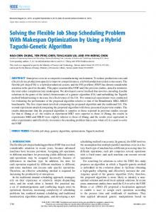
In this paper, an FMS which consists of a machining subsystem and an assembly subsystem is considered. These subsystems are linked by the material handling system, for example an Automated Guided Vehicle (AGV), as shown in Fig. 1. Consider a sample product P which is to be machined and then assembled (Fig. 2). It consists of two subassemblies sI and s2, and three parts p l ,p 2 ,and p 3 .Parts p I and p 2 are to be machined before the subassembly s1 is obtained. Assembling p3 and sIresults in the final product P (final subassembly s2 in Fig. 2 ) . The precedences among machining and assembly

1042-296X/89/0800-0451$01.00 @ 1989 IEEE

452

IEEE TRANSACTIONS ON ROBOTICS AND AUTOMATION, VOL. 5 , NO. 4, AUGUST 1989

+I

+ Part

p1

I

+ Part

p2

Subassembly

I I k

s,

P a r t ' pg

F i n a l subassembly

s2

Fig. 2. A sample product P.

Problem Name ~

Pattern

~~~

Single Product Scheduling Problem

0

N Product Scheduling Problem

N dtrttnct products

Fig. 3.

A digraph of the sample product P in Fig. 2.

Single Batch Scheduling Problem

0 0 o-..0

n identtcrl products

N Batch Scheduling Problem

Fig. 5 . Graphical illustration of four scheduling problems.

(a)

Fig. 4. Two different representations of the same product.

operations for the product can be represented by a directed graph (digraph) shown in Fig. 3. In this digraph, any node of degree 1, i.e., a node with the number of edges incident to the node equal to 1, denotes a part; and any node of degree greater than 1 denotes a subassembly or a final product. Another example of digraph is shown in Fig. 4(a). Without loss of generality, the representation of the digraph in Fig. 4(a) shown in Fig. 4(b) is used. The latter representation does not allow to assemble at a particular node more than one subassembly with any number of parts. At node s3 in Fig. 4(a), subassemblies sl, s2 and parts p 5 ,Pa are assembled. The same subassembly s3 has been obtained using the representation in Fig. 4(b), where an additional subassembly sI2was inserted. Four different aggregate scheduling problems are considered:

2) the N-product scheduling problem concerned with scheduling parts and subassemblies for N distinct products; 3) the single-batch scheduling problem concerned with scheduling parts and subassemblies for a batch of n identical products; 4) the N-batch scheduling problem concerned with scheduling of parts and subassemblies for N batches of products. Each of the above four problems is illustrated in Fig. 5. SCHEDULING PROBLEM 111. THESINGLE-PRODUCT

Consider a digraph representation of a product that consists of a number of parts and subassemblies. In the digraph each node is labeled (a, b, c), where a is the machining time, b is the assembly time, and c is the level of depth of node. The level of depth is assigned as follows: value of 0 is assigned to the root node (for example, node s2 in Fig. 3) and working backward from the root node to the initial nodes (i.e., nodes p l , p 2 , and p 3 ) values of increment 1 are assigned. The labeled digraph G from Fig. 3 is illustrated in Fig. 6. Before an algorithm for solving the single-product scheduling prob1) the single-product scheduling problem concerned with lem will be developed, a definition, l e m a , and two theorems scheduling parts and subassemblies of a single product; are presented.

KUSIAK: SCHEDULING OF A FLEXIBLE MACHINING AND ASSEMBLY SYSTEM

453

Fig. 6. A digraph with labeled nodes.

(b) Fig. 7. Examples of two types of digraphs. (a) Two simple digraphs G,. (b) Complex digraph.

Definition

Corollary

A simple digraph Gsis a digraph in which each node of a degree greater than 1 can have at most one preceding node of a degree greater than 1 (see Fig. 7(a)). Consequently, a complex digraph G is referred to a digraph that is not a simple digraph (see Fig. 7(b)).

If a subassembly represented by a complex digraph G can * g f and nodes be decomposed jnto subdigraphs gl’ g2 (parts) p l , p 2 , * * , ps by removing the root node uo, then

Lemma Any complex digraph can be decomposed into simple subdigraphs by removing a number of nodes corresponding to the final assembly or subassemblies.

-

C ( S ( g l ) ,S ( g 2 ) , S(gt),Pl,

*

S ( g j ) , S(gj+ 11,

S ( g t ) ,P I

9

e . . ,

>

* * * , P i , ~ i +- l* , * , ~ s )

5 C ( S ( g l ) ,S ( g z ) ,

i=l,

9

9

*

Pi-

* *

1,

9

S ( g j ) , Pi,

Pi+ I

s,j=O, 1,

e - . ,

*

9

S k j + I>,

* * * 9

~ s ) ,

t

The proof of the lemma is obvious and is not presented.

Theorem 1 (See Appendix I for the Proofl Scheduling nodes (parts or subassemblies) of G, with the Maximum Level of Depth First (MLDF) provides the minimum makespan schedule. Theorem 1 is illustrated in Fig. 8.

where S ( * ) is a schedule of subdigraph *, and C ( 0 ) is the makespan of schedule 0 . In the schedule h ~ in the ~ Gantt n chart in Fig. 8, two tYPeS of idle times are visible: in-process idle time I terminal time T.

454

IEEE TRANSACTIONS ON ROBOTICS AND AUTOMATION, VOL. 5 , NO. 4, AUGUST 1989

M

p2

p1

p4

p3

p5

I

'6 I

r

A

-

I

1

I 1 7

I I

I

I

1

1 ' 2 1

I

w

s2

-

-

I 1 I

TIME

s3

1

3

' I

T

i

schedule.

The in-process idle time refers to the assembly subsystem, whereas, the terminal time to the machining subsystem. Theorem 2 (See Appendix 11for the Proofl Consider a subassembly or final product P represented by a complex digraph G and decompose it into subdigraphs gl , g2, * , g,, by removing the root node uo of G. Let S*(gi) be the minimum makespan partial schedule associated with gi, i = 1, , t. If parts and subassemblies corresponding to gi and g, , i # j , are not preempted, then the minimum makespan schedule of product P is as follows:

-

where

S,(G)=[S*(g[l,), s*(&21),

* ' * Y

S*(g[kl)l, ITrjl for Iril

i

= 1,

- - -,k , is a schedule obtained using the Longest In-

process idle Time Last (LITL) rule SZ(G)= [S*(g[k+111, S*(g[k+2]), *

* *

3

s*k[tl)I, for Irjl > Tril

digraphs, set k = 0, and go to Step 3; otherwise, decompose each gl which is not a simple digraph into simple digraphs by removing its root node. Let uj denote a root node which has been removed, j = 1, * . ., J (note that the removed nodes should be numbered in increasing order starting from the root node of G). Set k = J and go to Step 3. Step 3. Let gik denote the simple subdigraph associated with u k . Use the MLDF rule to generate the minimum makespan partial schedule S * (gik) for each subdigraph gik, i = 1, * . ., Nk, where Nk is the number of subdigraphs obtained after uk has been removed. Step 4. For each partial schedule S * (gik) obtained in Step 3 determine i) in-process idle time I i k i ii) terminal time T,k,

1,

=

* - e ,

Nk.

Step 5 . Separate the S*(gik) into two lists: list 1: schedules S*(gjk) such that list 2: schedules S*(gik) such that

T.4 > Tk

Iik I Ijk

i = 1, .",Nk. Step 6. Use the LITL rule to generate

i = k + 1, k + 2, * t, is a schedule obtained using the Longest Terminal Time First (LTTF) rule. Based on Theorem 1 and Theorem 2, Algorithm 1 is developed.

Sl(gk)= [S*(g[l]k), S*(g[Z]k),

Algorithm 1 (The Single-Product Scheduling Problem)

SZ(gk)= [S*(g[i+Ilk), S*(g[r+Z]k),

*

9

S*(g[rlk)l,

a ,

Step 1. Label all nodes of the digraph G representing the structure of the product considered. If G is a simple digraph, then use the MLDF rule to generate optimal schedule of product P , stop; otherwise, go to Step 2. Step 2. Remove root node uo from G and decompose it into subdigraphs g!, I = 1, * , L. If all gl are simple

forS*(gik)inlist l , i = l , - " , r and use the LTTF rule to generate

forS*(gik)inlist2, i = r + l ,

e . . ,

* I

s*(g[flk)lr

t, t=Nk.

Then generate the partial schedule S*(gk)=[Sl(gk), S2(gk), u k l Step 7. If Uk = u o , then S * ( P ) = S*(go) is the optimal schedule, stop; otherwise, go to Step 8.

455

KUSIAK: SCHEDULING OF A FLEXIBLE MACHINING AND ASSEMBLY SYSTEM

g13

'23

g33

Fig. 9. Product P structure.

Fig. 10. The decomposed digraph G of Fig. 9.

Step 8. Consider S * ( g k ) as a simple subdigraph schedule and calculate Ik and Tk. Set k = k - 1, go to Step 3.

I

Algorithm 1 is illustrated in Example 1.

Example 1 Find the minimum makespan schedule for a product P , which has the structure of digraph G shown in Fig. 9. The values of machining and assembly times are as follows: Part number Machining time Subassembly number Assembly time

1 1 1 3

2 3 2 1

3 2 3 2

4 3 4 3

5 4 5 3

6 1 6 4

7 4 7 2

8 2 8 2

9 1 1 9 2

0 2 10 3

11 1 -

12 1 -

-

-

5

0

0

3

8

7

Step 1. Since the labeled digraph G in Fig. 9 is not a simple digraph, go to Step 2. Step 2 . Remove the root node u o , and nodes ul , u 2 , u3 so that the subdigraphs gll g21 g13 g23 g33 are obtained (Fig. 10). Step 3 . Use the MLDF rule to generate the partial schedules for the subdigraphs g13, g23, g33 associated with u3. The Gantt chart for each subdigraph is Fig. 1 1 . Gantt charts for the partial schedules for g,, ,g2,, and g,, in Fig. 10. shown in Fig. 11. Step 4. For each simple subdigraph, the in-process idle subdigraph gz3 is placed in list 1, g13 and g33 are placed in list 2. time and terminal time are Step 6. Use the LITL rule to generate I13=5, T 1 3 - 3 ; I23=3, T23=4; 3

I33=3, T33=2.

9

9

~ i ( g , ) = [ @ s~,

s6)i

9 ,

and use the LTTF rule to generate

Step 5 . Since: 113 > T13?

Y

I23

T23,

I33 > T33

SZ(g3)=[@6,

P7r SS), @IO,

PI19 S7)I-

456

IEEE TRANSACTIONS ON ROBOTICS AND AUTOMATION, VOL. 5 , NO. 4, AUGUST 1989

A

TIME

0

3

11

7 8

13

*I

4

0

15

Fig. 12. Partial schedule corresponding to the subdigraph with the root node uj in Fig. 10.

7

I

Mb, :oE p11 p12

7 s3 9

A

’5

I ’7

1‘8

[ ’9

TIME

In the last iteration, the above sequencing process is applied to uo and since

k list 2 : including S * ( P i )such that Zi 1, N. e . . ,

*

Z2


TI,

gl

is placed in list 2 .

e

*

>

T,, i = k

+

,

Step 3. For the schedules in list 1, develop the LITL schedule

457

KUSIAK: SCHEDULING OF A FLEXIBLE MACHINING AND ASSEMBLY SYSTEM

6'

A

0

3

II 7

'5

8

1 7' I

'8 1 ' 9

1

13

15

17

11

'1

152 2021

s4

s3

27

25

Fig. 15. Gantt chart of the minimum makespan schedule.

Step 4. Generate the final schedule S*(NP) = { S I( N P ) ,

(1,091)

S2("}.

-

TIME

sl0

> 30

33

(0,270)

Theorem 3 The schedule S * ( N P ) = { SI( N P ) ,S2( N P ) }generated by Algorithm 2 is the minimum makespan schedule of the Nproduct scheduling problem.

(3,0,1)

PRODUCT P I

The proof of Theorem 3 is similar to the proof of Theorem 2 except that the subdigraph gi is replaced by the digraph representing the product Pi. Algorithm 2 is illustrated in Example 2.

(2,0,2)

Example 2 Consider an N = 4 product scheduling problem. For simplicity, assume that the structure of each of the product can be represented by a simple digraph shown in Fig. 16.

(2,O.Z)

(0,3,0)

Step 1. Using Algorithm 1, the following schedules are obtained: Product P I : S * ( P l ) = { p l ,p 2 , s l } Product Pz: S*(P2) = ( ( ~ 3 ~, 4 SZ), , P S , ~ Product P3: S*(P3) = ( ( ~ 6 P, T , sd, pal ~

PRODUCT P2 3 )

9

,

s5 1

Product p4: S*(p4) = { P I o ,P I I Pi29 ,

s6).

The above schedules are illustrated in Fig. 17. Step 2 . From the Gantt charts in Fig. 17 the following data are obtained: List Product

1,

TZ

Number

PI

pz

4 6

p3

18

2 3 3

2 2 2

p4

9

10

1

Step 3 Using the LITL and LTTF rules results in the following schedules:

SI( N p )= [p41 S2("=[4,

p2, PI].

PRODUCT P4

Fig. 16. Structure of products P I ,P z . P3, and

P4.

458

IEEE TRANSACTIONS ON ROBOTICS AND AUTOMATION, VOL. 5 , NO. 4,AUGUST 1989

y

”; $

A

0

aN

4 6

”

u M

E-

H

3 0

0

*

3

&

A 0

4

7 9 1 2

A

h,TIME

0

9

19

Fig. 17. Schedules for products in Fig. 16.

Algorithm 2 can be used for solving the N-batch scheduling problem. The N-batch scheduling problem decomposes into N single-batch scheduling problems. Solution of this problem is illustrated in the example presented below. Example 3 Develop the optimal schedule S * ( N B ) for the N = 4 batch scheduling problem. The batch sizes of each product are as follows: Product

Batch Size

PI

PZ

2 2

p3

3 2

p4

Fig. 18. Simple digraph C , .

obtained. For the single-product scheduling problem with the complex digraph structure, the Longest Terminal Time First (LTTF) and the Longest Idle Time Last (LITL) rules combined with the MLDF rule generate the minimum makespan schedule. The rules developed for the single-product S*(NP)= (P4, P3, P2, P l ) . scheduling problem are applicable for solving the N-product , single-batch, and N-batch scheduling problems. Since each of The schedule S*(NB) obtained is as follows: the algorithms presented essentially involves sorting of a list of numbers, their computational time complexity is O ( n log n), where n is the length of the list. It should be emphasized that the aggregate schedules V. CONCLUSION generated by the algorithms discussed are used at the real-time In this paper, the following aggregate scheduling problems scheduling level discussed in Kusiak [ 113 and Kusiak and Chen [ 121. The real-time scheduling models consider all features of were considered: the automated manufacturing environment such as automated single-product scheduling problem material handling systems, fixtures, pallets, etc. N-product scheduling problem single-batch scheduling problem APPENDIX I N-batch scheduling problem. PROOF OF THEOREM 1 To solve the single-product scheduling problem, a simple Without loss of generality consider the two-level simple and complex digraphs were defined. It was shown that scheduling nodes with the Maximum Level of Depth First digraph G, in Fig. 18. Due to the precedence constraints between s1 and p a , , (MLDF) rule the optimal schedule for the single-product scheduling problem with the simple digraph structure was Pd, and between s2 and p l , * * * , pn,scheduling nodes of the

The structure of each product is shown in Fig. 16. Using Algorithm 2 results in the following schedule (see Example 2 ) :

459

KUSIAK: SCHEDULING OF A FLEXIBLE MACHINING AND ASSEMBLY SYSTEM

digraph according to the MLDF rule result in the following makespan:

n

+max

W ) - C tb;),0 ) i= I

where t(*)is the processing time of a part or subassembly 0 . For any P k , k = 1, 2, . . * , n, scheduled before pi, j = a, * d, the makespan can be expressed as follows: a ,

It is clear that C

IC,,

k

= 1,

2,

. . e ,

n.

APPENDIX I1 PROOF OF THEOREM 2 The proof of Theorem 2 follows the following conclusion presented in Kurisu [lo]: An optimal schedule for a two-machine string problem can be derived based on the fact that string i precedes string j , if min ( a ; ,bj)