Aggregation Supportive Authentication in Wireless ... - Semantic Scholar

Aggregation Supportive Authentication in Wireless Sensor Networks: A Watermark Based Approach Wei Zhang, Yonghe Liu, and Sajal K. Das Center for Research in Wireless Mobility and Networking(CREWMAN) Department of Computer Science and Engineering, The University of Texas at Arlington Arlington, TX 76019 Email: {wzhang, yonghe, das}@cse.uta.edu Abstract— In-network processing presents a critical challenge for data authentication in wireless sensor networks (WSNs). Current schemes relying on message authentication code (MAC) cannot provide natural support for this operation since even a slight modification to the data invalidates the MAC. In this paper, based on digital watermarking, we propose an end-to-end approach for data authentication in WSNs that provides inherent support for in-network processing. In this scheme, authentication information is modulated as watermark and superposed to the sensory data at the sensor nodes. The watermarked data can be aggregated by the intermediate nodes without incurring any en-route checking. Upon reception of the sensory data, possibly distorted by the operations along the route, the data sink is able to authenticate the data by validating the watermark, detecting whether the data has been altered and where it has occurred. In this way, the aggregation–survivable authentication information is only added at the sources and checked by the data sink, without any involvement of intermediate nodes. Furthermore, the simple operation of watermark embedding and complex operation of watermark detection provide a natural solution of function partitioning between the resource limited sensor nodes and resource abundant data sink. The simulation results show that the proposed scheme can successfully authenticate the sensory data with high confidence.

I. I NTRODUCTION Due to severe resource limitations and hence limited defense capabilities on a sensor node, authenticating the sensory data gathered by a wireless sensor network is crucial for a plethora of mission critical applications [20, 21, 23]. While extensive efforts have been devoted toward this purpose in conventional networks, the unique characteristics of wireless sensor networks (WSNs) have often prevented their direct adoptions. One of the key challenges for authentication in WSNs is to provide natural support for in-network processing, a main feature operation in WSNs. Given potentially large amount of sensory data, to reduce network load and hence preserve energy, numerous schemes [8, 11] have been proposed to employ in-network processing for aggregating the sensory data gathered by multiple sensor nodes on their en-route path toward the data sink (or sink). These schemes, however, have dictated conventional end-to-end authentication (the sink’s capability to directly authenticate the sensory data from sensor nodes) infeasible, as the data may have been modified legitimately along the route by intermediate nodes due to aggregation. Correspondingly, a set of papers have proposed en-route data authentication based on message authentication code (MAC) [20, 21, 23]. Usually, a sensor node shall append a

1-4244-0992-6/07/$25.00 © 2007 IEEE

MAC to its sensory data or to an aggregate report as an endorsement. These MACs will then be checked by the intermediate nodes along the route to the sink. Thanks to the simplicity of MAC operation, the intermediate nodes are capable of detecting/discarding tampered data in an energy efficient way in terms of both computation and communication. However, the high frequency of MAC checking, associated with complicate peer-to-peer key management schemes, often dramatically increases the overall system complexity. In addition, when there are multiple compromised intermediate nodes, these schemes are subject to failure. Motivated thereby, we propose an authentication scheme for WSNs that renders end-to-end checking (sensor–to–sink) capability without relying on any intermediate nodes, while still compatible with in-network aggregation. Our scheme is based on digital watermarking, a proven technique notably in the multimedia domain. Our key idea is to visualize the sensory data gathered from the whole network at a certain time snapshot as an image, in which every sensor node is viewed as a pixel with its sensory reading representing the pixel’s intensity. As a result, digital watermarking can be applied to this “sensory data image”. Specifically, we adopt direct spread spectrum sequence (DSSS) based watermarking to balance energy consumption in the network with asymmetric resources. With a simple mathematical operation (addition), each sensor node can embed part of the whole watermark into its sensory data, while leaving the heavy computation load from watermark detection at the sink. At the same time, the robustness of DSSS technology enables our scheme to survive certain degree of distortion and thus naturally supports innetwork aggregation. Once the aggregated and watermarked data reaches the sink, the sink is able to verify the existence of the watermark and hence the authenticity of the data. The remainder of this paper is organized as follows. Section II summarizes the related work. In Section III, we introduce the preliminaries and our system model. The watermarking based authentication scheme is detailed in Section IV. Section V discusses some specific design issues that occur in WSNs. Section VI presents the simulation results. We conclude the paper in Section VII. II. R ELATED WORK A set of papers have employed MAC for data authentication in WSNs [20, 21, 23]. Notably among them are en-route MAC

checking schemes against the false data injection. In these schemes, an aggregated report is often endorsed by multiple nodes’ MAC. These MACs will then be verified along the forwarding route either in a statistical manner [20], or in an interleaved hop-by-hop fashion [23], or through the Hill Climbing approach [21]. While providing the desired authenticity, these schemes demand the establishment of complex key schemes for pairwise MAC verification. Moreover, the nature of MAC itself excludes any in-network processing on the data as it will inevitably result in invalid MACs. Another set of works [15, 19], including ourselves [22] have been focusing on secure in-network processing, which often employ techniques exemplified by statistical estimation, interactive commit and proof, and trust model. The focus of these techniques is securing aggregation results and do not directly address authentication issue. While watermarking has been the subject intensively studied in multimedia domain [10, 18], in particular, for digital right management, rarely has it been used in WSNs [5]. In [5], digital watermark is embedded into WSNs in the form of nonlinear programming, where the additional constraints are used to embed watermarks. While this solution can be utilized in certain applications such as localization, the special formulation may limit its application to other domains. In contrast, our work directly applies the watermark on the sensory data, which enables a much broader application. III. P RELIMINARIES A. Architecture and system model We consider a densely deployed WSN monitoring certain physical environments, where the network is hierarchically organized into a two-tier cluster structure through some clustering algorithms such as LEACH [8]. Within each cluster, sensor nodes periodically report their sensory data to the cluster head. The cluster head in turn aggregates and forwards the results to the sink. In addition, we assume that each sensor node knows its own location and all sensors’ clocks are synchronized using some existing schemes, like [16] and [7]. The reported data hence can be location- and time- stamped. We consider one of the key objectives of such WSN is to understand sensing field of the covered area, e.g., the temperature distribution in a particular field. To achieve this, a cluster head will perform aggregation on all its members’ data and report to the sink. In order to retain the specifics of the collected data, commonly used, but highly abstract aggregation functions, such as Max/Min, Average etc., are not employed. Instead, the cluster head will compress all the gathered data and transfer to the sink. Based on the compressed data from multiple cluster heads, the sink will be able to reconstruct the desired information for further analysis, for example, to build spatial–temporal models of the sensing field. B. In-network processing/aggregation As mentioned before, the aggregation function in our model is beyond simple scalar operations, such as Max/Min, etc. To monitor the whole sensing field, we can visualize it as an image, where every single node is viewed as a pixel, with the

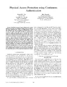
sensory data as the pixel’s intensity. Naturally, we can adopt the existing image compression schemes as the aggregation functions to reduce network load while retaining the desired details of the data. Since our main purpose is not to develop any new compression algorithm, in the remainder of the paper, we employ JPEG-like compression approach for illustration purpose. For JPEG [6], an object (e.g. an image) is first divided into a number of non-overlapping blocks. Then, a linear transform, such as Discrete Cosine Transform (DCT) or Discrete Wavelet Transform (DWT), is applied to each block to transform the data into frequency domain. The coefficients of different frequencies are further quantized based on certain metric. Finally, these quantized coefficients, most of which are zero, are encoded by entropy coding with the smallest number of bits. We adopt this compression method as our aggregation operation. Based on the block size (system parameter), a cluster is first divided into blocks in each of which, DCT is performed by the cluster head. Unlike JPEG employing a quantization matrix derived from Human Visual System, the transformed coefficients here are quantized through K-largest coding [6], where only the K-largest coefficients in each block are kept while the rest are discarded. Finally, the quantized coefficients are encoded using Huffman coding. We remark that these techniques are well studied and our adoption at this level is direct and for the purpose of compression only. C. Digital watermarking Digital watermarking technology has been widely adopted to protect copyright ownership of multimedia [2, 4]. The key idea is to hide certain information about the multimedia material within that material itself. As illustrated in Fig. 1, a generic watermarking system is usually composed of two components: an embedder and a detector [4]. The embedder takes three inputs: 1) messages that are encoded as the watermark; 2) cover data that are used to embed the watermark; and 3) key that is optional for enforcing secure watermark generation. As an embedder’s output, the watermarked data is distributed. When it is presented as the detector’s input, with the key information (depending on whether employed), the detector can determine whether a watermark exists and decode it. Cover data Watermark

Watermark embedder

( Key )

Fig. 1.

Watermarked data

Watermark detector

Detected watermark

( Key )

Generic watermarking system

The watermark detection schemes can be categorized to two classes: informed detection, where the original cover data is accessible; and blind detection, where the original cover data is not required. The type of watermark can be as fragile, robust and semi-fragile. Fragile watermarks will become invalid after even the slightest changes to the cover data. Robust watermarks can survive moderate to severe distortion on the cover data while semi-fragile watermark is in between [4].

watermark detection: watermark (+1,-1,-1,+1) exist??

When applying watermarking in WSNs, as the sensory data is not available at the sink beforehand, blind detection is a must. At the same time, the lossy nature of wireless environment, and legitimate distortion due to in-network processing prevents the use of fragile watermarks. Therefore, in our scheme, we adopt robustness, blind detection based watermarking.

data sink

compressed data 22 0 -4 0 24 0 0 0 0 0 0 0 -11 6 0 0 0 0 0 0 0 0 0 0 4 0 0 0 0 0 0 0 cluster head

IV. WATERMARK BASED S ENSORY DATA AUTHENTICATION Intuitively, a snapshot of all readings from the sensor nodes can be visualized as an image representing the whole sensing field, where each node is analogous to a pixel and its reading indicates the pixel’s intensity. Therefore, we can embed watermark in this image in a distributed fashion at each node. Given the watermark as a prior knowledge, the sink is then able to verify the integrity of the sensory data. Furthermore, as the watermark is designed to be tolerable of compression, the scheme can co-exist with in-network processing. In this section, we present our scheme in a regular network where sensors are deployed in a grid topology and describe watermark embedding and detection operations. The practical issues specific in WSNs will be addressed in Section V. A. Overview For the conventional watermarking, the whole image is available for the embedder to manipulate the watermarks. Unfortunately, it does not hold in WSNs since a single sensor node may only know its own data while lacking of a global view of the “sensory data image”. Therefore, the watermark in our scheme is embedded in a distributed fashion by each node. Our solution is illustrated in Fig. 2. In this scheme, each sensor node is assigned a small (compared to the sensory data), i.i.d. random value as its watermark. This random value is then added to the sensory reading before sending to the cluster head. Once the cluster head receives the data, it compresses them and routes to the sink. With the knowledge of the random value added at each sensor node, the sink can calculate the inner product of this random sequence composed of random values with the received sensory data. By evaluating the obtained value to determine the presence of watermark, the sink will be able to authenticate the sensory data and pinpoint whether and where illegitimate modification has occurred. Essentially, our scheme employs the principle of DSSS: while each sensor node only modifies its data by an invisible value, adding up a large number of the squares of these values will give a significant gain. On the contrary, without knowing the embedded values, the modifications will appear to be noise and go undetectable to an attacker. Next, we will describe the watermark embedding and detection scheme in detail. B. Watermark generation and embedding Our work is inspired by [10, 18], both of which map watermarking into modulation schemes in the conventional communication system. Under such mapping, an image is

restored data 20 21 21 20 18 22 19 23 21 24 24 21 20 24 21 19 25 28 24 23 23 25 26 30 28 26 25 23 28 25 28 32

In-net processing: compression transmitted watermarked data 22 25 22 22 20 23 20 19 20 22 19 18 21 22 19 22 21 24 27 21 23 25 26 30 23 25 21 24 26 23 24 34

+1

-1

-1

+1

sensor nodes

watermark embedding original sensing data 20 21 21 20 18 22 19 23 21 24 24 21 20 24 21 19 25 28 24 23 23 25 26 30 28 26 25 23 28 25 28 32

Fig. 2. Illustration of the watermarking scheme: based on the assigned watermark, each sensor node will report a modified sensory reading. This watermarked data will then be compressed at the cluster head. While the watermark may be distorted during this process, the sink can still validate the presence of the watermark and hence authenticate the data.

approximated as a continuous, two-dimensional, band-limited channel, where the original unmodified image is treated as noise with high power while the low power signal is the watermark. The essence is spread spectrum [14]: the signal is spread across a wide range of frequencies so that the signal power is ultra low at a particular frequency. The low signalto-noise ratio reduces the chance that an attacker detects the signal (watermark) to enforce security, while at the same time, the wide frequency of the signal carrier augments robustness to compression. Since even compression may remove a fraction of the signal from the whole frequencies, most of signal should still remain due to the fact that the signal energy resides in all frequency bands. In order to directly add the spreading sequence (watermark) at each individual sensor node in the spatial domain, DSSS is employed in our work. Let (x, y) be the 2-D coordinate representing the position of a sensor node. Without confusion, we also simply use (x, y) to denote the corresponding sensor node. Let S denote the set of all sensor nodes. To embed L bits [b1 , b2 , · · · , bL ], (bi ∈ {−1, 1}, i ∈ [1, L]) as watermark into the sensory data, the sink first divides the sensor nodes into L non-overlapping subsets, S = {S1 , S2 , . . . , SL }, such that Si ∩ Sj = ∅, ∀i 6= j, (i, j ∈ [1, L]). That is, for each single watermark bit bi , it is spread into its corresponding subset Si . For each Si , the sink will generate a binary, pseudorandom variable s(x, y) ∈ {−1, 1} for each node. Notice that this random s(x, y) is indexed to each node and hence each subset Si contains a pseudorandom sequence {s(x, y)|(x, y) ∈ Si }. In addition, the sink will generate a random value α(x, y) for each node to denotes the maximal allowable distortion toward the sensory reading. α(x, y) equals to the amplitude of the watermark for node (x, y) and how to determine its value will be discussed in Section V-A. Thus the watermark for sensor

node (x, y) ∈ Si is defined as

(

w(x, y) = bi α(x, y)s(x, y).

δij =

We assume that this value can be securely assigned to sensor node (x, y). This can be achieved through secure broadcast or unicast, like [13] for sample solution. Given w(x, y) and sensory data o(x, y), sensor node (x, y) will simply report d(x, y) = w(x, y) + o(x, y) as its watermarked sensory data. Fig. 3 illustrates how the watermark is embedded in each individual sensor node. Suppose we have two watermark bits, b1 = 1 and b2 = −1, to be embedded. So, the 8 sensor nodes n1 , n2 , . . . , n8 are divided into two subsets, S1 and S2 , where n1 , . . . , n4 ∈ S1 and n5 , . . . , n8 ∈ S2 . All the nodes in the same subset are designated the same bit (b1 or b2 ) so that the watermark is applied to all sensory data. Within each subset, a pseudorandom binary variable s and random variable α is assigned to each individual node. As an example, for sensor node n1 , its s and α is +1 and 2, respectively. As a result, n1 ’s watermark is (+1) ∗ 2 ∗ (+1) = 2. After adding this to its original sensory data which is 20, n1 then reports 22 as its watermarked data to its cluster head.

1, 0,

i=j i 6= j

Here, ||φi ||2 can be considered as the average power of φi and is determined by α(X, Y ). When each sensor node modifies its data to embed watermark as described above, the complete watermark w of the whole image composed of all nodes can be expressed as, L X

w(X, Y ) =

bi φi (X, Y ),

where bi ∈ {−1, 1} is the watermark bit and (X, Y ) is the set of all sensor nodes. Fig. 4 demonstrates the network-wise watermark embedding process. It can be seen that dividing the sensors into non-overlapping subsets guarantees the orthogonality of the modulation pulses. The whole watermark in the network is the superposition of all the bits modulated by each pulse. Since each sensor just changes its data by a small amount, the overall modification on the sensing filed will not significantly affect the modeling process at the data sink.

20

n1

n2

n5

n6

(+1, +1, 2)

(+1, +1, 4)

(-1, -1, 1)

(-1, -1, 2)

22

21

n3

21

(+1, -1, 1)

25

21

n4

20

24

22

20

n7

(+1, -1, 2)

22

24

secret bit bi

(-1, +1, 5)

b1 = +1 b2 = −1

21

(-1, +1, 3)

pseudorandom sequence s

Fig. 3.

18

random variable α

watermarked transmitted data

Watermark embedding in individual sensor node

We call φi a modulation pulse used to modulate one watermark bit and {φi } should be orthogonal with each other, i.e., X x,y

24 24

W=

∑bφ

i i

i



=

2

 −1

 21 

4

S2

2 4 0 0    −1 − 2 0 0 

φ1 :  1

2

S1

S2

0 −1 − 2  5 3  0 0 0

φ2 : 

 Watermarked data  22    O+W:  20

− 2 − 5 − 3 

25 22 22  

22 19 18 

Network-wise watermarking

C. Watermark detection with in-network compression

For ease of later mathematical manipulation, we rephrase the above description with a few new symbols to fit it in communication terms. While using the 2-D coordinate (x, y) to represent a particular sensor node, (X, Y ) is a set of sensor nodes. Let φi be the random sequence assigned to subset Si , where ( α(X, Y )s(X, Y ), (X, Y ) ∈ Si φi (X, Y ) = (1) 0, otherwise

< φi , φj >=

 21

Fig. 4.

sensor node original sensing data

21 21 20 

22

n8

19

 20

original data O:  

S2 b2: -1 sequence s: {-1, -1, +1, +1} randomα {1, 2, 5, 3}

(2)

i=1

S1 S1 b1: +1 sequence s: {+1, +1, -1, -1} random α {2, 4, 1, 2}

.

φi (x, y)φj (x, y) = ||φi ||2 δij = ||φj ||2 δij

After compressed at the cluster head, the watermarked data will be routed to the sink. There, the data is projected on each modulation pulse φi to obtain the correlation coefficients. By deriving the statistical characteristics of the correlation coefficients, the watermark detection process can formulated as a binary hypothesis testing. The presence of watermark indicates the authenticity of the sensory data while absence of watermark will alarm possible attacks. Let dQ , oQ and wQ represent the restored watermarked data, sensing data and watermark after compression/quantization respectively. The correlation coefficients is calculated as ri =< dQ , φi >=< wQ , φi > + < oQ , φi > + < e, φi > . As dQ = (o + w)Q 6= oQ + wQ , e represents the non-linear quantization error introduced by compression, which can be approximated as i.i.d. random variables. Due to the randomness of modulation pulses, < oQ , φi >, < wQ , φi > and < e, φi > can be considered as random variables. According to the central limit theorem, the sum of such random variables ri should follow Gaussian distribution. Moreover, with multiple pulses modulating multiple watermark bits, all the correlation coefficients form a jointly

Gaussian distribution. A general Gaussian problem of hypothesis testing on correlation coefficients is formulated as [1] ( H1 : R = W + N, watermark present . H0 : R = N, watermark not present where, the correlation coefficients vector R = Q Q T φ ] [r1 , r2 , . . . ...rL ]T , W = [b1 φQ φ , b φ φ , . . . b φ 1 2 2 L L 1 2 L Q Q Q and the noise vector N = [(o + e)φ1 , (o + e)φ2 , . . . , (o + e)φL ]T . For the statistical characteristics of each correlation coefficient ri , the first-order and second-order moments of ri can be derived as [9] PL P Q Q α α i=1 ||φ · φi || E[ri |H1 ] ' bi = bi = bi ∗ xi , (3) L L P Q where xi = α α/L for all ri , i ∈ [1, L]. And P Q 2 2 (o ) α (αQ )2 α2 V ar[ri |H1 ] = σ 2 = + (E[s4 ] − 1). (4) L L Similarly, the characteristics of correlation coefficients without watermark can be derived as P Q 2 2 (o ) α 2 E[ri |H0 ] = 0, and V ar(ri |H0 ]) = σ0 = . L With the statistical characteristics of the correlation coefficients under both H1 and H0 available, we can perform hypothesis testing. Let m1 and m0 be the mean vectors under hypotheses H1 and H0 respectively, that is, mj = E[R|Hj ], (j = 0, 1). And the covariance matrices are [1]: Cj = E[(R − mj )(R − mj )T |Hj ], (j = 0, 1). To simplify the analysis, the pseudorandom sequence s is chosen to meet E[s4 ] = 1 so that the covariance matrices C1 and C0 are same. Then the logarithm likelihood ratio test is 1 1 (R−m0 )T C−1 (R−m0 )− (R−m1 )T C−1 (R−m1 ) ≷ γ 2 2 (5) Because the correlation coefficients ri is uncorrelated with each other, the cross-covariance is negligible compared to the covariance. Therefore, the covariance matrix can be approximated as C = σ 2 I. After some mathematical manipulations, the sufficient statistic T(R) is: 1 (m1 − m0 )T R ≷ γ 0 (6) σ2 According to Neyman-Pearson criterion [1], for a fixed false alarm probability PF , we can derive the threshold for a watermark to be detected. Specifically, based on the definition of PF : T(R) =

T(R) − mT ) PF (T(R)|H0 ) = erf c1 ( p var[T(R)] we can get

p T(R) = erf c−1 (PF ) var[T(R)] + mT

(7)

T(R) is a linear combination of Gaussian random variables, so it is also a Gaussian random variable. We have 1 erfc, √2 π

complementary error function, is defined as erfc(x) = R ∞ called −t2 dt x e

mT = E[T(R)|H0 ] = 0

(8)

var[T(R)|H0 ] = (m1 − m0 )T C−1 (m1 − m0 )

(9)

and

Substituting Equ. (8) and (9) into (7), and combining Equ. (4) and (6), the watermark detection condition is expressed as L X

√ bi ri ≷ erf c−1 (PF )σ L

(10)

i=1

The above formula is used at the sink to determine whether or not the watermarks present in the reported data. If the left side is bigger than the right side, the sink will consider watermark present, otherwise, watermark is not present. V. P RACTICAL C HALLENGES AND D ISCUSSION In the above discussion, we consider a basic scenario and have omitted some key practical design issues, such as, network capacity in terms of watermark amplitude and number of bits, the irregularity of sensor deployment. In this section, we focus on these practical challenges when applying the above watermarking scheme in WSNs. A. Network capacity Increasing the watermark amplitude and embedded bits can leverage detection and thus enhance security. For a network that embeds L information bits, there are M = 2L combinations for a brute force attack to determine the actually embedded bits. Intuitively, the more secret bits embedded in a network, the more secure the network gains. However, a network cannot unlimitedly embed watermarks. In our watermarking scheme, from the detection viewpoint, the watermark is the true signal while the sensory data can be viewed as noise. According to Shannon’s channel capacity theory, the upper bound of watermark bits that can be embedded in a network is given as: L = C log2 (1+SN R), where C is the total available bandwidth and SNR is the ratio of signal to noise power [17, 18]. In our case, C is the total number of nodes in the network since the watermark is spread to every sensor node. Let ∆m and ∆o be the average of watermark amplitude and sensory data respectively, then SN R in our case equals to: ∆2m /∆2o . By changing the log base from 2 to e and applying series expansion, the above equation can be simplified as [24]: L/C ≈ 1.433 ∗ SN R.

(11)

Equ. (11) shows that raising the watermark amplitude ∆m can increase SNR and further the number of watermark bits. Notice that unlike in image domain – where the watermark amplitude is confined by the Human Visual System, the constraints in WSNs are different. So, taking WSNs’ characteristics into account, we will discuss what is the suitable watermark amplitude and how many watermark bits can be embedded. A.1 Watermark amplitude

Intuitively, two factors determine the watermark amplitude: security constraints and system accuracy requirement. The former factor assures that an adversary cannot infer the watermark when it overhears the watermarked data and the latter one guarantees that the embedded watermark does not compromise the applications’ desired data accuracy. i) Security constraints For the attackers who know that the sensory data has been watermarked, the security constraints will prevent attackers from deriving the embedded watermark even if they are monitoring the same environment. Considering an adversary with the same sensing capability as the legitimate ones is close to some sensor nodes, if the watermark amplitude is too large, the adversary can derive the watermark by comparing the watermarked data with certain reasonable guess of the true sensory data based on its own reading. Moreover, if an adversary can eavesdrop all the packets from different sensor nodes around him, inappropriately large watermark is vulnerable for statistic analysis. The adversary may first average all the watermarked data and then compares every data with the average to trace watermark. To overcome these vulnerabilities, the watermarked data should be disguised as “regular data”, so that an adversary cannot easily conjecture from its own readings. In other words, compared with the original (unwatermarked) data, the watermark should look like a “reasonable” sensory error. Toward this end, we construct a secure magnitude bound ∆s within which the watermark is undetectable by attackers. Obviously, ∆s may vary from applications. Here, we adopt a general sensing model [12] to derive the watermark bound from the security viewpoint. Let os be the received signal by sensor s from the radiating source op located at p. Then, the relation between the received signal and the original source is os = se(s, p)op + e

(12)

where e is the noise and se(s, p) is the sensibility. Equ. (12) shows that for two nodes at different locations (x1 , y1 ) and (x2 , y2 ), two factors cause their readings different: measurement error (e) and sensibility (se) attenuation introduced by the distance between (x1 , y1 ) and (x2 , y2 ). Therefore, we can estimate the magnitude of each factor and combine them to obtain the security watermark bound ∆s . The measurement error e is inherited in each sampling and determined by sensors’ sensing capabilities. Due to the measurement error, even for the same monitoring environment, the repeatedly readings from a single sensor or a single reading from multiple sensors may be different. Without loss of generality, the distribution of measurement error for all nodes in homogeneous WSNs can be assumed as Gaussian distribution: e ∼ N (0, σs2m ). σs2m can be estimated from sensor manufacturer’s specifications and adjusted by field measurements. To simulate the measurement error and exploit it as the watermark, the sink shall generate N random variables following Gaussian distribution N (0, σs2m ) and assign each to one sensor with the magnitude, ∆sm . In addition, since sensors’ sensing ability diminishes with distance, the distance factor could also be another source to

hide watermark. Depending on the distance between each sensor and the sensing point, different sensors may have various readings. So, we can utilize it to increase the watermark magnitude. Considering that we know the sensing field area A and the total number of deployed sensor nodes Z, then the density of the network is A/Z. If we assume the homogenous sensors are uniformly deployed such that each sensor is located at the center of a square grid, then the p average distance between each node can be approximated to A/Z. Therefore, some measurements may be performedpto estimate the sensibility attenuation by the distance of A/Z and calculate the error ∆sdis introduced by sensibility attenuation. Combining the above two factors together, the watermark amplitude should be: ∆s ≤ ∆sm + ∆sdis . Under this condition, the watermarked data shall remain “consistent” with the normal sensory data – even by the judgment from an adversary who has its own measurements of the same environment. ii) System accuracy requirement ∆s defines the average watermark amplitude under security constraints. Besides, the application-dependent accuracy requirement also restricts the watermark amplitude. Although from the watermark detection point of view, the original sensory data is considered as noise, its value cannot be distorted too much by the watermark since it is the true demand of WSNs applications. Therefore, the original data amplitude should dominate both before and after compression to commit the desirable accuracy. Assuming ∆a is a network’s total tolerable error, three main error sources contribute to ∆a : measurement error (∆m ), p watermark error (∆wa ) and distortion error (∆c ). So, ∆a = ∆2m + ∆2wa + ∆2c . Among them, the measurement error ∆m , which equals to ∆sm , has been discussed before. Watermark error ∆wa introduced by the embedded watermark is determined by the watermark amplitude. Distortion error ∆c comes from lossy compression. Therefore, according to the network accuracy p requirement, the watermark amplitude should be: ∆wa = ∆2a − ∆2m − ∆2c . Combining both security and accuracy requirements, the final watermark amplitude ∆m should be ∆m = min(∆s , ∆wa ).

(13)

∆m indicates the average watermark amplitude that can be embedded in sensor nodes which in turn determines the value of α(x, y) in Equ. (1). For a given ∆m , there are different ways to embed the watermarks which can lead to various outcomes from Equ. (11). Next, we will compare the number of watermark bits that can be embedded for different embedding schemes and the tradeoffs between them. A.2 Number of watermark bits The watermark embedding scheme described in Section IVB (called scheme I in later discussion) partitions the whole network into several subsets, each of which spreads one watermark bit. The orthogonality of the modulation pulses φi is realized as the positions of nodes to spread the watermark bit in each pulse (non-zero part) are different with each other. The net effect of such scheme is that for each sensor node,

it is only modulated by one single pulse. Therefore, ∆w is applicable to every sensor node, thus SN R1 = ∆2m /∆2o and the total number of watermark bits is L1 ≈ 1.433∗C ∗SN R1 . Besides this non-overlapping partition scheme, the modulation pulses can also be generated by orthogonal pseudorandom sequence generator. Let φ0i be the orthogonal binary sequences generated by some code generator, whose each bit is assigned to one sensor node. For one watermark bit bi , another watermark P embedding scheme (called scheme II) would be w0 = α0 bi ∗ φ0i , where α0 represents the tolerable watermark distortion. In this scheme, there is no zero part in each modulation pulse φ0i . Considering each single sensor node corresponds to an index of every modulation pulse, it carries the sum of all pulses at that particular index. As P an example, for node (x, y), its modulation value would be i bi ∗ φ0i (x, y). Different with scheme I, if the bits from all the pulses happen to be same for node (x, y), the modulated watermark value at (x, y) will be multiplied by the total number of pulses. Therefore, α0 or ∆0m shall be the acceptable distortion of the aggregate of all pulses. To ensure no node’s watermark exceeding the watermark amplitude ∆m , when there are L2 bits to be embedded via L2 pulses, ∆0m should be ∆m√ /L2 . So for scheme II, √SN R2 = (∆m /L2 )2 /∆2o and L2 ≈ 3 1.433 ∗ C ∗ SN R1 = 3 L1 . It can be seen that for a given watermark amplitude ∆m , the watermark bits from scheme II is cube root of scheme I because it reduces the applicable watermark amplitude to compensate the aggregate of all modulation pulses on one node. Although this scheme decreases the network capacity in term of the number of watermark bits, it brings some desirable advantages. Comparing with scheme I, where each sensor node modifies its sensory data by amplitude of ∆m , for scheme II, only some nodes whose modulation bits happen to be same for all pulses change their data to that amount. For the rest nodes, their modification may be much smaller than ∆m or even be zero. Therefore, the total distortion introduced by watermark is smaller than scheme I. For example, we did some tests. To embed two watermark bits with ∆m /∆o = 0.25, 32 and 96 nodes are needed for scheme I scheme II, respectively. Assuming that the sensory data in both schemes following N (20, 4), for a compression ratio of 3.2 (keeping 5 largest coefficients for every 4 ∗ 4 block), the watermark distortion measured by mean square error(MSE) is 30 vs. 20 for scheme I and scheme II. B. Block formulation for irregular sensor deployment Until now, we have assumed regular deployment of sensor nodes in a grid topology. Under this assumption, data compression can be relatively easy as the sensory data naturally forms a regular image pattern. However, if sensor nodes are irregularly deployed in a random fashion, the cluster head must divide the nodes to equal size blocks before compression. We remark that the block formulation here is implemented by each cluster head for compression purpose. So it is not related to the subset division in Section IV, which is performed by the sink to spread watermark bits. Notice that one subset may span two or more clusters and depending on the density,

it is also possible that there are more than one subsets within one cluster. To divide the sensor nodes into blocks of size m, a system parameter, we develop a 2D tree based partition algorithm. Our 2D tree based approach, which is essentially similar with the KD-tree concept [3], utilizes both x- and y- coordinates alternately to partition the node set. For each partition, it generates either a block of size m or an almost balanced binary tree. Therefore, the physically proximate nodes are likely assigned into a same block. Since the statistical properties do not substantially differ in adjacent nodes, such partition benefits the compression ratio. Generally, given the cluster members’ locations and the total number of sensors within one cluster, the cluster head first determines the number of blocks n based on block size m. If the total number of sensor nodes is not a multiple of block size, the cluster head will add “padding nodes” by duplicating certain randomly chosen nodes. Then, depending on the parity of the number of blocks, the cluster head bisects the nodes (even number blocks case) or “pre-divides” m nodes (odd number blocks case) with a vertical or horizontal line. The algorithm is described in Algorithm 1. WSNPartion (P , depth, m, n) Input: A set of nodes P (including pads), current depth depth, block size m and number of blocks needs to be partitioned n. Output: A binary tree storing P . if number of blocks n is odd then if depth is even then split P into two subsets with a vertical line l. Let P1 be the set of left of l including the m leftmost points in P . Let P2 be the right of l including the rest; vlef t P1 ; vright WSNPartion (P2 , depth + 1, m, n − 1); end else split P into two subsets with a horizontal line l. Let P1 is the set of left of l including the m topmost points in P , and let P2 be the right of l including the rest; vlef t P1 ; vright WSNPartion (P2 , depth + 1, m, n − 1); end end else if depth is even then split P into two subsets with a vertical line l through the median x-coordinate of the points in P . Let P1 be the set of points to the left of l or on l, and let P2 be the set of points to the right of l; end else split P into two subsets with a horizontal line l through the median y-coordinate of the points in P . Let P1 be the set of points above l or on l, and let P2 be the set of points below l; end vlef t WSNPartion (P1 , depth + 1, m, n/2); vright WSNPartion (P2 , depth + 1, m, n/2); end create a node v storing l, make vlef t the left child of v and make vright the right child of v; return v

Algorithm 1: Partition Algorithm Formally, given a set of nodes P (including the padding nodes) and the block size m, the cluster head first sorts x- and y- coordinate values for all nodes. If the number of blocks n is odd, the algorithm first splits the set P with a vertical line l on x-coordinate into two parts, Plef t and Pright . The resulting Plef t includes m leftmost nodes and Pright includes the rest nodes. This operation is termed “pre-division”. The vertical

splitting line is stored at the cluster head and Plef t is stored in the left subtree and Pright is kept in the right subtree. If the number of nodes in Pright is greater than the block size m, Pright is further split into two subsets of roughly the same size by a horizontal line: the nodes above or on the line are stored in the left subtree of Pright and the points below it are stored in the right subtree of Pright . Similarly, for each resulting subtree, depending on whether the remaining number of block is odd or even, each subtree either performs ”predivision” or split it into two roughly equal size subsets. This procedure will then be repeated until each subtree has exactly m nodes. Fig. 5 illustrates how the partition is performed and the corresponding binary tree. For ease of illustration, m is set to 2, i.e., each block shall have two nodes. l1

predivide

l1 l1

l1

n=2

P2 P1

l2

l2 P1

P1

P2

P2

P3

n=2

n=3

l1 P1

P2

predivide

l1

P3

l3

l2

l1

l1

P2 l3

n=4 P3 P1

l2

l2

P1

P4

P3

P2

P1

P2

P3

l2 P1

P4

P4

l2 l4

l3

P5 P2

l4

n=4

P3

P4

P5

n=5

predivide

l1 P4

P1

predivide

l1

n=3

n=3 l4

l2

l4

l2

P1 P2

l3

P3

Fig. 5.

P5

P6

l5

P4

l3 P2

P3

l5 P5

P6

n=6

Partition the network into blocks

After the partitioning terminates, the blocks composed of sensor nodes have been formed. During the runtime, if some node gets dysfunctional due to either out of battery or other reasons, the cluster head will average all its neighbors’ readings as a padding value.

the watermark detection probability with different network sizes and compression ratios. Then, considering that the possible attacks may occur both before and after aggregation, a set of simulations are performed in spatial and frequency domain respectively. A. Simulation setup To focus on the attacks’ effects on watermark, we follow the general compression process and assume that the irregular deployed sensor nodes haven been formed into blocks using the partition algorithm described in Section V-B. Specifically, the cluster size and block size is same, which equals to 64. Within each cluster, the cluster head first performs 8 ∗ 8 DCT. Unless otherwise specified, there are totally 4096 sensor nodes in the whole network, so there are totally 64 blocks/clusters in the network. The default compression ratio is 90%, that is, in one block/cluster, the 7 largest DCT coefficients including the DC component are kept and others are set to zero. For the whole network, a random variable following Gaussian distribution N (20, 4) is generated and assigned to each sensor nodes as its realtime sensory data. Within one cluster, one watermark bit is spread by a pseudorandom modulation pulse generated by Hadamard code. Therefore, 64 watermark bits in total are embedded in the whole network. The allowable distortion toward the sensory reading (α) follows Gaussian distribution N (3.5, 1). Referring to Equ. 1, we employ “tiled version spread” scheme [18] which means that the same pseudorandom sequence is used for all φi while the non-zero portion’s location is different for each φi . A data sink samples 2000 rounds during each simulation and each simulation is repeated 5 times. B. Effects of network size and compression rate In this section, we investigate the performance of the proposed watermark based scheme when there is no attack. Two factors are considered here: network size and compression rate.

C. Remnant check We claim that the presence of watermark is only necessary but not sufficient condition for authentication. An example of undetectable attack would be simply enlarging all the sensory data, which causes the reinforcement on the watermark (note: an adversary is unlike to reduce the sensory data since it will automatically decrease the watermark). To detect this attack, “remnant check” are performed after the hypothesis testing claiming the presence of watermark. Generally speaking, after extracting the watermark from the restored data to obtain the “remnant”, the sink shall project it again on each modulation pulse. Presence of apparent correlation and repetitive detection of the watermark will indicate such attack has been launched. Fig. 6.

Effects of network size and compression rate

VI. S IMULATION S TUDY In this section, we evaluate the performance of the proposed scheme under different possible attacks. First, we investigate

In Fig. 6, the detection probability is the probability that the proposed scheme authenticates the data properly. It can

C. Attacks in spatial domain An attack may be launched during the transmission from the sensor nodes to their cluster head. For this kind of attack, an attacker directly modifies the sensory data. Since the ultimate goal of our applications is modeling the whole sensing field which requires that the cluster head to report all the data after compression. As a result, just modifying any particular sensing data does not result in an effective attack. Instead, an attacker may aim to alter as many nodes as possible. 1) False distribution imposition on all sensor nodes: To disturb correctly modeling the whole sensing field, instead of counterfeiting a single sensory data, an attacker could impose certain false distributions upon the sensory data to deceive the sink. Here, two most common distributions, Gaussian and uniform distribution, with different parameters are examined. Fig. 7 shows the detection probabilities under different bogus distributions. In which, the bogus Gaussian distribution is with different mean values and a fixed standard deviation of 4, e.g. N (2, 4), N (3, 4), . . . , N (10, 4). 1 Gaussian Uniform

Detection probability

0.8

0.6

0.4

0.2

0

2

3

Fig. 7.

4

5 6 7 Mean of bogus distribution

8

9

10

Bogus Gaussian distribution

It can be seen that the scheme is able to correctly detection the attack when the mean value of the bogus Gaussian distribution is bigger than 4, which equals to 20% of the

original data amplitude. In fact, for the bogus distribution with mean value of 3, the scheme is most likely detect it (> 90%). Fig. 7 also shows the detection probabilities under uniform bogus distribution with different mean values and fixed range of 4 (with an exception for the case with mean value of 2). That is, U[1, 3], U[1, 5], U[2, 6], . . . , U[8, 12]. Compared to Gaussian distribution, with the same mean value, the detection probability in this case is much lower. For example, for the mean value of 2, the detection probability is 0.1 for uniform attack while 0.6 for Gaussian. That is because unlike the Gaussian distribution where most forged data is close to the mean value, the false data (within some range) in this case is uniformly distributed among the sensory data, this randomness has weak “pattern” from the watermark decoder’s point of view and contributes to the lower detection probability. However, as the mean value of the uniform distribution increase to 5 (25% of the original data), this scheme is capable of detecting the attack with zero miss probability. 2) False distribution imposition on part of sensor nodes: In addition to disguising a bogus distribution onto a whole network, the bogus distribution may be just imposed to some sensor nodes. Fig. 8 shows the detection probability when a bogus Gaussian distribution N (5, 4) is imposed on the different numbers of random selected nodes. 1

0.8

Detection probability

be seen that in general, the bigger the network size is, the higher detection probability. That is because with the network size increasing, there are more watermark bits that can be embedded. Therefore, the statistical characteristic of the general Gaussian problem can be more precisely represented, which in turn improves the accuracy of the hypothesis testing. The compression rate in the figure is the ratio of the DCT coefficients set to zero to the total number of DCT coefficients in one block. Since the higher compression rate will introduce more data distortion, the detection probability drops as the compression rate increases. This simulation result verifies that the watermark in this scheme is robust to compression, which is a prerequisite for our aggregation-supportive, end-to-end authentication approach. As shown in the figure, for the network size of 64 ∗ 64 and with the compression rate of 90%, the scheme is still able to fully detect the watermark.

0.6

0.4

0.2

0 10

Fig. 8.

15

20 30 Percentage of modified nodes (%)

50

70

Bogus Gaussian distribution on random selected nodes

Fig. 8 indicates that the detection probability exceeds 0.7 when there are 20% of total nodes whose data get modified. When the number of attacked nodes reaches to 30%, the likelihood of detection is a very high (> 0.97). As mentioned before, the sensory data from any single node is not main interest for data modeling, the scheme fits the requirement since when a moderate number of nodes (e.g. 20 − 30%) get compromised, the proposed scheme can successfully detect it by authenticating the embedded watermark. 3) Remnant check: Besides camouflaging another distribution on the sensory data, an attacker may also alter all the sensory to a certain extent. Although this kind of attack would be rare and not sensible in multimedia domain, it could be an easy but disastrous threat in WSNs. “Remnant check” described in Section V-C can effectively defend such attack. Here, the performance under both possible scenarios (increasing or decreasing the sensory data value) is evaluated. In Fig. 9(a), the x-axis is the modified data amplitude on scale of the original sensory data. It can be seen that the

0.8

0.8

0.6

0.4

0.2

0 120

2) Non-zero coefficients position switch: Instead of changing the values, a compromised cluster head may switch the positions of nonzero coefficients with zero ones after quantization. The simulation results indicate that our scheme can detect such attack with 100% of detection probability without any missing occurs.

0.6

0.4

0.2

125

130

135 Data value (%)

140

160

0 20

180

(a) Increase sensory data

40

60

65 Data value (%)

70

75

80

(b) Decrease sensory data

Fig. 9.

Remnant check

scheme is not very sensitive for detection when the degree of change is not severe, e.g., when the modified data is less than 1.4 times of the original one for increase case (Fig. 9(a)), or bigger than 0.75 times of original for decrease case (Fig. 9(b)). However, with the degree of the alteration aggravating, the correlation between the remnant data and the watermark becomes stronger. Thus, our scheme can quickly detect it so that the detection probability approaches to 1 for the other cases. Therefore, our scheme works well when an attacker considerably alters the sensing data. D. Attacks in frequency domain Upon aggregation/compression, the sensory data is transformed into frequency domain by the cluster head and the quantized coefficients are transferred to the sink. Therefore, a compromised cluster head or any intermediate nodes that are along the path between the cluster head to the sink may modify the transform coefficients to launch an attack. 1) Coefficients value forgery: Similar with the spatial domain, the value of the transform coefficients could be counterfeited. Fig. 10 shows the detection probability when the quantized transform coefficients are modified by a different extent. 1

1

0.8

Detection probability

Detection probability

0.8

0.6

0.4

0.2

0 120

0.6

0.4

0.2

125

130 135 Coefficients value (%)

140

(a) Increase coefficients Fig. 10.

160

0

40

60

65 70 Coefficient value (%)

75

80

(b) Decrease coefficients Frequency coefficients attack

Fig. 10 shows that the detection probability under frequency attack is very close to the cases in the remnant check (Fig. 9). That is because that DCT is a linear operation, that is, DCT (a ∗ X) = a ∗ DCT (X). Therefore, the net effect on coefficients modification is essentially same as that in spatial domain which leads to the detection probability is consistent with that in Section VI-C.3

E. Node failure Besides these above attacks, another issue for aggregation is node failure, either due to physical damage or battery depletion. This case can be handled by two ways: the value of the fault node is set zero or is averaged by its neighbors. Since node failure is unavoidable in WSNs, when the total fault nodes is minority in the network, the network is still considered workable. However, when majority of nodes are failed, the gathered information is not much valuable for modeling. 1 average zero 0.8

Detection probability

1

Detection probability

Detection probability

1

0.6

0.4

0.2

0

5

10

15 20 node failure (%)

Fig. 11.

30

50

Node failure

The watermark detection probability under different percentage of the fault nodes is shown in Fig. 11. In Fig. 11, “zero” means to leave the fault node reading as zero while “average” means to average the sensory readings from the fault node’s four neighbors (up, down, left, right) as its reading. The results in Fig. 11 meet the above requirements. It shows when the percentage of node failure reaches 15%, the gathered data will fail the watermark based authentication. The rational lies in that from the data sink point of view, it is the cluster head that modifies the data source, thus breaking the authentication. Moreover, compared with “average”, the “zero” case is more subject to detect when there are minor node failure in the network. VII. C ONCLUSION In this paper, we propose a watermarking based authentication scheme for wireless sensor networks. The distinct advantage of the proposed scheme is to achieve end-to-end authentication where the sink can directly validate the sensory data from the sources. At the same time, the approach provides natural support for in-network processing as it is robust to the distortion introduced therein. Our design is in particular suitable for applications in the resource limited environment

as the watermarking embedding process is simple and highly energy efficient. The simulation results verify that the proposed scheme can achieve compression survival authentication. ACKNOWLEDGMENT This work is supported by NSF grant # IIS-0326505 and Texas ARP grant No. 14-748779. R EFERENCES [1] M. Barkat, Signal Detection and Estimation, Second Edition, Artech House, 2005. [2] M. Barni, F. Bartolini, Watermarking Systems Engineering: Enabling Digital Assets Security and Other Applications Marcel Dekker, 2004. [3] M. Berg, M. Kreveld, M. Overmars and O. Schwarzkopf, Computational Geometry: Algorithms and Applications, Second Edition, SpringerVerlag, 2000. [4] I. Cox, M. Miller, and J. Bloom, Digital Watermarking, Morgan Kaufmann, 2002. [5] J. Feng and M. Potkonjak, “Real-time Watermarking Techniques for Sensor Networks”, ES&T/SPIE, Security and watermarking of Multimedia Contents, Santa Clara, CA, Jan., 2003. [6] R. C. Gonzalez and R. E. Woods, Digital Image Processing , Prentice Hall, 2002. [7] J. Greunen and J. Rabaey, “Lightweight Time Synchronization for Sensor Networks”, in Proceeding of (WSNA), San Diego, Sep. 2003. [8] W. R. Heinzelman, A. Chandrakasan, and H. Balakrishnan, “EnergyEfficient Communication Protocol for Wireless Microsensor Networks,” in Proceedings of Int’l Conference on System Sciences (HICSS), 2000, p. 8020. [9] J. R. Hernandez, and F. Perez-Gonzalez, “Statistical Analysis of Watermarking Schemes for Copyright Protection of Images”, in Proceedings of the IEEE, Special Issue on Identification and Protection of Multimedia Information, vol. 87, no. 7, pp. 1142-1165, Jul., 1999. [10] J. Hernandez, F. Perez-Gonzalez, J. Rodriguez and G. Nieto, “Performance Analysis of a 2-D-Multipulse Amplitude Modulation Scheme for Data Hiding and Watermarking of Still Images”, in IEEE Journal on Selected Areas in Communications, vol. 16, No. 4, pp. 510-524, 1998. [11] C. Intanagonwiwat, R. Govindan and D. Estrin, “Directed Diffusion: A Scalable and Robust Communication Paradigm for Sensor Networks”, in Proceedings of the Int’l Conference on Mobile Computing and Networking (MobiCom), Boston, MA, Aug. 2000. [12] S. Meguerdichian, F. Koushanfar, G. Qu and M. Potkonjak, “Exposure in Wireless Ad-Hoc Sensor Networks“, in Proceeding of the 7th ACM Seventh Annual International Conference on Mobile Computing and Networking (MobiCOM ’01), 2001. [13] A. Perrig, R. Szewczyck, V. Wen, D. Culler, and D. Tygar, “Spins: Security Protocols for Sensor Networks”, in Proceedings of the Seventh Annual Int’l Conference on Mobile Computing and Networking (ACM MOBICOM ’01), Rome, Italy, 2001, pp. 189–199. [14] R. Pickholtz, D. Schilling and L. Milstein, “Theory of SpreadSpectrum Communications – A Tutorial”, in IEEE Transactions on Communications, vol. 30, No. 5, pp. 855-884, 1982. [15] B. Przydatek, D. Song and A. Perrig, “SIA: Secure Information Aggregation in Sensor Networks”, in Proceedings of ACM SenSys, Los Angeles, CA, Nov. 2003, pp. 255-265. [16] A. Savvides and M. Strivastava, “Distributed Fine-Grained Localization in Ad-hoc Networks of Sensors”, in Proceedings of the Seventh Annual International Conference on Mobile Computing and Networking (ACM MOBICOM ’01), Rome, Italy, 2001. [17] C. E. Shannon and W. W. Weaver, The Mathematical Theory of Communication, The University of Illinois Press, Urbana, Illinois, 1963. [18] J. R. Smith, and B. O. Comiskey, “Modulation and Information Hiding in Images”, in Proceedings of Int’l Workshop on Information Hiding, 1996, pp. 207-226. [19] D. Wagner, “Resilient Aggregation in Sensor Networks”, in Proceedings of the 2nd ACM workshop on Security of Ad hoc and Sensor Networks (SASN), Washington DC, 2004, pp. 78-87. [20] F. Ye, H. Luo, S. Lu, and L. Zhang, “Statistical En-Route Filtering of Injected False Data in Sensor Networks”, in Proceedings of IEEE INFOCOM, HongKong, 2004. [21] Z. Yu and Y. Guan, “A Dynamic En-route Scheme for Filtering False Data in Wireless Sensor Networks”, in Proceedings of IEEE INFOCOM, Barcelona, Spain, Apr., 2006.

[22] W. Zhang, S. Das and Y. Liu, “A Trust Based Framework for Secure Data Aggregation in Wireless Sensor Networks”, in Proceedings of IEEE SECON, Reston, VA, Sept., 2006. [23] S. Zhu, S. Setia, S. Jajodia and P. Ning, “An Interleaved Hop-by-Hop Authentication Scheme for Filtering of Injected False Data in Sensor Networks”, in Proceedings of IEEE Symposium on Security and Privacy, Oakland, CA, 2004, pp. 260-272. [24] “An Introduction to Direct-Sequence Spread-Spectrum Communications“, http://pdfserv.maxim-ic.com/en/an/AN1890.pdf.