A. Simulation of a Boeing B737-700 flight. In this experiment, the aircraft mass m is set to be 60000 kg and the thrust setting η is set to be 0.96. The actual.
Aircraft Mass and Thrust Estimation Using Recursive Bayesian Method Junzi Sun1 , Henk A.P. Blom1,2 , Joost Ellerbroek1 , and Jacco M. Hoekstra1 1
Faculty of Aerospace Engineering, Delft University of Technology, the Netherlands 2 Air Transport Safety Institute, National Aerospace Laboratory, the Netherlands
Abstract—This paper focuses on estimating aircraft mass and thrust setting using a recursive Bayesian method called particle filtering. The method is based on a nonlinear state-space system derived from aircraft point-mass performance models. Using solely ADS-B and Mode-S data, flight states such as position, velocity, and wind speed are collected and used for the estimation. An important aspect of particle filtering is noise modeling. Four noise models are proposed in this paper based on the native ADS-B Navigation Accuracy Category (NAC) parameters. Simulations, experiments, and validation, based on a number of flights are carried out to test the theory. As a result, convergence of the estimation can usually be obtained within 30 seconds for any climbing flight. The method proposed in this paper not only provides final estimates, but also defines the limits of noise above which estimation of mass and thrust becomes impossible. When validated with a dataset consisting of the measured true mass and thrust of 50 Cessna Citation II flights, the stochastic recursive Bayesian approach proposed in this paper yields a mean absolute error of 4.6%. Keywords - aircraft, state estimation, point-mass model, measurement noise, particle filter, Bayesian estimation
I. I NTRODUCTION Estimating aircraft mass based on observed flight trajectory data has long been a topic of interest in ATM research. Aircraft mass acts as not only as an important parameter for many different studies of aircraft performance, but is also a desired piece of knowledge for air traffic controllers in practice. Airlines, however, treat this data as confidential, and access is rarely given to either researchers or air traffic controllers. In practice, this means this data is not accessible nor actively used by the research community. Earlier studies that addressed this problem were commonly focused on deterministic methods based on the aircraft total energy model (TEM), which is also the core of the BADA performance calculation [1]. Alligier et al. presented a leastsquares method [2] and a follow-on machine learning method [3]. Around the same time, Schultz et al. implemented an adaptive estimation method to estimate the aircraft mass [4]. These methods used accurate radar data for estimation. In our previous studies, we also proposed two different approaches based on ADS-B data. The first study made use of the data from the takeoff phase [5]. The second method used Bayesian inference to construct a posteriori estimation by combining masses computed from different flight phases [6]. From all these studies, a strong link between aircraft mass and thrust setting is evident, and it is not possible to estimate one of the two parameters without some knowledge of the other. Most of the aforementioned studies essentially addressed the estimation process as an optimization problem. Their solutions are obtained using a form of least-squares fitting. Aircraft mass estimated under these conditions is often unrealistic and even outside plausible physical boundaries. This is often due to the uncertainty in the trajectory data, as well as the uncertainty in the system equations. Although the effect of noise is an important aspect in the entire inference process, its relation to mass estimation has not yet been studied comprehensively by previous studies. It is therefore one of the main contributions of this paper.
The problem of mass estimation by a (ground-based) observer can be considered as having to solve an inversed nonlinear multi-state system using noisy observation data. To tackle this complex system, we constructed a detailed point-mass flight performance model with ten system states and eight observables in this paper. Then, a tailored, Sample Importance Re-sampling (SIR) particle filter, is introduced to solve these system equations. In addition, four different levels of observation noise models are constructed, based on ADS-B navigation accuracy standards, which are used in the particle filtering. Both simulated and real flights are used to test the model and method. After that, a set of actual flight data with known initial mass are used for validation. Finally, the paper also offers conclusions on the relationships between estimation and uncertainties based on our model and method. The remainder of the paper is structured as follows. Section two describes the fundamentals of recursive Bayesian theory, particle filtering, the point-mass flight dynamic system equations, noise models, and the detailed algorithm. Section three presents our experiments using simulated and real flight data. Section four offers the validation results based on real flight data. Finally, a discussion and conclusions are presented in sections five and six. II. R ECURSIVE BAYESIAN ESTIMATION AND ITS APPLICATION TO AIRCRAFT STATE ESTIMATION
Aircraft flight dynamics are complex, non-linear, and multivariate. Estimation of parameters such as mass depends on solving this fairly complex inversed flight dynamic system. Due to the high non-linearity and number of system states, deriving the estimation of mass under noisy measurements (and thrust setting when possible) is the main goal of this section. To this end, we will first give a fundamental introduction to the use of the recursive Bayesian method for generic system state estimation. The Sample Importance Re-sampling (SIR) particle filtering method is introduced for the estimation purposes. Then, the specific system of aircraft flight dynamic equations will be addressed. Combining with the SIR, the solution for the system will be given. A detailed algorithm implementation will also be provided. This section will end with the definition of the observation noise models and other stochastic elements of the SIR. Recursive Bayesian estimation is a probabilistic method for system states filtering, prediction, and estimation. One of the most widely used applications is the Particle Filter, which is technically known as the Sequential Monte Carlo Method. Starting for a set of initial state conditions, the recursive Bayesian determines the values for the next set of states based on the joint posterior probability of all previous states’ measurements. Commonly, for non-linear system with a large number of states, the computation of a closed-form joint posterior probability is not practical. For this reason, the Monte Carlo method is introduced. It utilizes a very large number of weighted particles to approximate the true probability density functions, where each particle represents a possible set of state values. Through a stochastic update and sampling processes, the original challenge
ICRAT 2018
of updating a high-dimensional joint posterior probability is then transformed to adapting the weights of particles. A. Recursive Bayesian estimation First, it is crucial to explain the basics of how recursive Bayesian theory is used for system state estimation. Denoting xt as the system states and yt as observables at time t ( t ∈ N ), the evolution of the discrete-time state model and observation model of a system can be generalized as follows: xt = f (xt−1 , νt−1 ) yt = h(xt , nt )
(1)
where f and h represent the state transition function and observation function, νt is the process noise, and nt is the observation noise. νt and nt are assumed to be mutually independent sequence of independent and identically distributed variables. Equation 1 represents the general case of the system and observation function for recursive Bayesian methods. In the particular case of this paper, we assume an additive Gaussian model for both process noise and observation noise. We further assume the noises extends linearly and equation 1 is rewritten as xt = f (xt−1 ) + νt−1 yt = h(xt ) + nt
p(yt |xt )p(xt |y1:t−1 ) p(yt |y1:t−1 )
(3)
where the first part p(yt |xt ) is the measuring probability that can be computed based on observation noise n. Due to Equation 2, xt is a first order Markov process, hence the second part p(xt |y1:t−1 ) becomes: Z p(xt |y1:t−1 ) =
p(xt |xt−1 )p(xt−1 |y1:t−1 ) dxt−1
p(xt |y1:t ) ≈
(4)
where the first term p(xt |xt−1 ) is the state transition probability. It can be computed by the system transaction equation based on the process noise model ν. Combining the above two equations, the recursive form becomes: p(yt |xt )p(xt |xt−1 ) p(xt−1 |y1:t−1 ) dxt−1 p(yt |y1:t−1 ) (5) where the denominator of the fraction is a normalizing factor which does not need to be computed explicitly. The difficulty is to compute the measuring probability and transition probability. In most cases an analyticity solution is not possible. That’s where Sequential Monte Carlo (SMC) simulation comes to work. Z
p(xt |y1:t ) =
B. Particle filtering A particle filter is a recursive Bayesian estimator based on importance sampling that computes the posterior density in a Monte Carlo fashion. It approximates the target distribution p(x) using a large number of samples (particles), drawn from an proposal distribution q(x) and updates it recursively. To describe the SMC process, at time t, let {xit , wti }N i=i be state particles that can represent the posterior density
N X
wti δ(xit )
(6)
i=1
where δ(·) is a Dirac delta function centered at xit and wi is the normalized weight of a particle which satisfies wi = p(xi )/q(xi ). The most important part of particle filtering is the measurement updating. Sequentially, the particle weight wti is updated in a recursive form. The solution is presented in Equation 7, as derived in [7] : xit ∼ q(xit |xit−1 , y1:t ) p(yt |xit )p(xit |xit−1 ) i w ˜ ti ∝ wt−1 q(xit |xit−1 , y1:t ) w ˜i wti = PN t ˜ ti i=1 w
(7)
At each iteration, the sum of all weights is normalized to one as shown in the last equation. The posterior filtered density is approximated using Equation 6. We can also compute the expected value of the states at each time step using the particle weights:
(2)
Regardless of the form of system and observation functions, the goal of filtering is to compute the probability of system states at any time t based on the observation from time 1 to time t, denoted as p(xt |y1:t ). p(xt |y1:t ) =
p(xt |y1:t ), where {xit } is the set of states with weights {wti }. Henceforth, the posterior density is approximated with the empirical probability density:
E[xt ] =
N X
xit wti
(8)
i=1
There are different ways to choose the proposal distribution. A specific particle filter - Sample Importance Re-sampling (SIR) - is used for solving the problem of this paper. The SIR particle filter uses the state transition distribution p(xt |xit−1 ) as the proposal distribution q(xt |xit−1 , yk ). Therefore, the particle update equations in Equation 7 can be simplified as: xit ∼ p(xit |xit−1 ) wti ∝ p(yt |xit )
(9)
For a SIR particle filter, an additional re-sampling process at each iteration is included. The re-sampling step generates a new set of particles based on the approximated p(xit |xit−1 ). Weights of all particles are also assigned to 1/N after the re-sampling. This step is essentially a redistribution of particles, which replaces low-weight particles with high-weight particles. The standard re-sampling algorithm is called residual re-sampling, which was proposed by Liu et al. in 1998 [8]. Other forms of re-sampling such as systematic re-sampling and stratified resampling are summarized by Douc and Cappe in 2005 [9]. In this paper, residual re-sampling is used. III. S YSTEM OF POINT- MASS AIRCRAFT PERFORMANCE MODEL
A. Aircraft state In previous section, the general form of the state system and solution using particle filter were given. In this section, the specific system equations based on point-mass aircraft performance are proposed. To illustrate, Figure 1 shows the observable states in all three axes. The left figure shows a horizontal projection of a trajectory, and the right figure a vertical projection. For ease of computation, latitudes, longitudes, and altitudes are converted to a reference Cartesian coordinate system. Denoting aircraft mass as m, thrust setting coefficient as η, distance flown as ~s, altitude as z, ground speed as ~vg , true airspeed as ~va (in horizontal projection), vertical rate as (vz ), and wind speed as ~vw , the system state x vector is:
ICRAT 2018 Y ψ va χ
ωv
Z w
vz
vg
y
γ
z
vg x
X
x
X
Fig. 1: Observed states in the flight dynamic system
x = (m, η, ~s, z, ~vg , ~va , vz , ~vw )
(10)
The vector variables in corresponding x and y axes components are:
Lt
=
vt
=
mg qt 2 + (v )2 va,t z,t
(25) (26)
where L, and D are lift and drag force, and ρ and S are the air density and the aircraft wing surface. From the BADA model [1], T is the maximum thrust profile defined by three coefficients. Cd0 and k are coefficients for zero drag and induced drag respectively. During real flights, not all thrust settings can be used for any aircraft mass. The reduction of thrust has a lower limit depending on actual aircraft mass. In the particle filter, such constrains are introduced as the initialization of the particles. The following Equation 27 is adapted from BADA [1] and is used to constrain the relation of mass and thrust setting. η ∈ [ηmin , 1]
~s = (x, y) ~vg = (vgx , vgy ) ~va = (vax , vay ) ~vw = (vwx , vwy )
ηmin = 1 − 0.20 · (11)
Additional angular parameters in Figure 1 are flight path angle γ, ground track χ, aircraft heading ψ, and wind direction φ. The measurement vector y is represented as: y = (~s˜, z˜, ~v˜g , v˜z , ~v˜w )
(12)
B. State evolution Since the goal is to model the system as accurately as possible and shift the uncertainty to the observation noise model, when possible we assume zero process noise for mt , ηt , ~st , zt , and ~va,t . For states that the perfect process model cannot establish accurately (or are unknown), we use an autoregressive model to describe their process equations. These states are the vertical rate vz and wind ~vw . The complete state process equations can be described as follows: mt ηt ~st zt ~va,t vz,t ~vw,t
= mt−1 = ηt−1 = ~st−1 + (~va,t−1 + ~vw,t−1 ) dt = zt−1 + vz,t−1 dt = ~va,t−1 + ~at−1 dt = αvz vz,t−1 + εvz = α ~ w~vw,t−1 + ~εw
(13) (14) (15) (16) (17) (18) (19)
where ~at is the horizontal acceleration. State updates for vz and ~vw are expressed using two autoregressive (AR) models with lag p = 1. Parameters αvz , εvz , εw , and α ~ w are estimated using the least-squares method. The detailed process and results are shown in Section III-D. To compute the acceleration (~at ) at each time step, we need to consider the forces acting on the aircraft. The equations used at each time step are listed as follows:
mmax − m mmax − mmin
(27)
C. Modeling the aircraft measurement noise Measurement noise is closely related to sensor errors. For example, GPS errors affect position measurements (related to state x ˜) and altimeter errors affect altitude measurements (˜ z ). Besides sensor errors, the truncation of values in downlinked data (such as latitude, longitude, and altitude in ADS-B position messages) also contributes to the measurement error. ADS-B transponders operate under regulations that define the minimum accuracy of sensors [10]. Different categories of uncertainty indicators are transmitted through ADS-B. In this paper, the Navigation Accuracy Categories (NAC) are considered for the construction of observation noise models. In Table I, the Navigation Accuracy Category - velocity (NACv) defines the level of accuracy in terms of horizontal and vertical speed. The NACv indicator is broadcast within the airborne velocity message (Type Code 18). HFOM and VFOM, short for horizontal and vertical figure of merit, indicate the 95% confidence interval which is translated as twice of standard 2 , deviation in the observation noise model. They define the σvg 2 2 σva , and σvz . TABLE I: Navigation Accuracy Category / Velocity NACv 4 3 2 1 0
HFOM