Algebraic Constraints on Initial Values of Differential Equations

Algebraic Constraints on Initial Values of Differential Equations F. Leon Pritchard, York College; William Sit, City College, CUNY

May 8, 2009 Graduate Center Series Kolchin Seminar in Differential Algebra,

F. Leon Pritchard, York College; William Sit, City College,CUNY Algebraic Constraints on Initial Values of Differential Equations

Abstract • Objects: Systems of ordinary differential equations which are ♦ polynomial in the unknown functions and their derivatives. • Method: Study the differential consequences of algebraic ♦ constraints on the initial value domain by an inductive but finite process, and exploiting the quasi-linearity of such consequences. • Goals: To compute algebraic constraints on the initial ♦ conditions, and when possible, an explicit representation of the vector field, such that on the set determined by the constraint equations (and inequations), the initial value problem of the original system of differential equations can be solved uniquely by solving the explicit system. F. Leon Pritchard, York College; William Sit, City College,CUNY Algebraic Constraints on Initial Values of Differential Equations

A Quasi-Linear Example • z1 (t), z2 (t), z3 (t) are functions of t ♦ • z˙1 (t), z˙2 (t), z˙3 (t) are their derivatives with respect to t ♦ −z2 z˙1 z3 z˙1

− z2 z˙2 + z1 z˙3 + 2z˙3 2 + z1 z˙2 − z1 z˙2 + z˙3

= z14 = 5z3 = 3z22 = z3

• Algebraic constraints found by symbolic computation: ♦ z12 = z2 , z13 = z3 . • Explicit representation found by symbolic computation: ♦ z˙1 =

z3 , z2

z˙2 = 2z2 ,

z˙3 = 3z3 ,

z2 6= 0.

F. Leon Pritchard, York College; William Sit, City College,CUNY Algebraic Constraints on Initial Values of Differential Equations

Questions

• Who have been studying these problems? ♦ • Where are the difficulties? ♦ • What determines the set of consistent initial values? ♦ • When is the solution unique? ♦ • When does an explicit form z˙ = r (z) exist? ♦ • How can symbolic methods help? ♦ F. Leon Pritchard, York College; William Sit, City College,CUNY Algebraic Constraints on Initial Values of Differential Equations

Theoretical Developments • Campbell (1980,1985,1987), Campbell and Gear (1995), ♦ Campbell and Griepentrog (1995) Gear and Petzold (1983,1984), Gear (1988, 2006), Reich (1988, 1989): G. Thomas (1996, 1997), J. Tuomela (1997, 1998) singularities, constant rank conditions, linear and differentiation index • Rabier and Rheinboldt (1991, 1994, 1996): ♦ general existence and uniquenss theory for differential-algebraic systems on π-submanifolds • Kunkel and Mehrmann (1994, 1996, 2006): ♦ local invariants, strangeness index, and canonical forms for linear systems with variable coefficients, numerical solutions F. Leon Pritchard, York College; William Sit, City College,CUNY Algebraic Constraints on Initial Values of Differential Equations

Numerical Methods

• difficulties with implicit, unprocessed, high index systems: ♦ constant rank condition, and stability • Campbell (1987): ♦ reduce index through differentiations, drift-off • Kunkel and Mehrmann (1996a, 1996b): ♦ numerical methods requiring a priori knowledge of local and/or global invariants

F. Leon Pritchard, York College; William Sit, City College,CUNY Algebraic Constraints on Initial Values of Differential Equations

Recent Approaches • Campbell and Griepentrog (1995): ♦ combining symbolic with numerical methods • Thomas (1996): ♦ symbolic computation of differential index for quasi-linear systems based on algebraic geometry and prolongation • Thomas (1997), Rabier and Rheinboldt (1994b) : ♦ singularities, impasse points • Tuomela (1997a): ♦ regularizing singular systems with jet spaces F. Leon Pritchard, York College; William Sit, City College,CUNY Algebraic Constraints on Initial Values of Differential Equations

Contents • transformations to quasi-linear systems ♦ • the concepts of essential degree and algebraic index and ♦ algorithms to compute these • algorithms for prolongation and completion ♦ • generalized concepts of quasi-linearity ♦ • sufficient conditions for existence and uniqueness theorem ♦ • algorithm to compute constraints on initial conditions ♦ • algorithm to compute explicit vector field ♦ • examples and implementation in Axiom ♦ F. Leon Pritchard, York College; William Sit, City College,CUNY Algebraic Constraints on Initial Values of Differential Equations

Set Up • z = (z1 , . . . , zn ): indeterminate functions of t ♦

• z˙ = (z˙1 , . . . , z˙n ): their derivatives with respect to t ♦ • x0 : a point in Cn , complex n-space ♦

• (X, P) = (X1 , . . . .Xn , P1 , . . . , Pn ): algebraic indeterminates ♦ • f1 , . . . , fm : polynomials in X, P over C ♦ • Initial value problem: ♦

f1 (z1 , . . . , zn , z˙1 , . . . , z˙ n ) = 0, .. . fm (z1 , . . . , zn , z˙1 , . . . , z˙ n ) = 0, z(0) = x0 . F. Leon Pritchard, York College; William Sit, City College,CUNY Algebraic Constraints on Initial Values of Differential Equations

Explicit Representation, Rational Form

A system is explicit or explicitly given if m > n and f1 , . . . , fm have the form fi = Pi − ri (X), fn+k ∈ C[X],

where ri (X) ∈ C(X) for 1 6 i 6 n, for 1 6 k 6 m − n.

• Write ri (X) = Ri (X)/S(X) with a common denominator S(X) ♦

F. Leon Pritchard, York College; William Sit, City College,CUNY Algebraic Constraints on Initial Values of Differential Equations

Explicit Representation, Polynomial Form • Introduce new indeterminates X0 , P0 . ♦ • Equivalent system: gi ∈ C[X0 , X, P0, P] for 1 6 i 6 m + 2 ♦ gi = Pi − X0 Ri (X)

for 1 6 i 6 n, for 1 6 k 6 m − n,

gn+k = fn+k gm+1 = X0 S(X) − 1, gm+2 = P0 + X03

n X ∂S(X) i =1

∂Xi

Ri (X).

F. Leon Pritchard, York College; William Sit, City College,CUNY Algebraic Constraints on Initial Values of Differential Equations

Basic Transformations

• Non-autonomous to autonomous ♦ • High order to first order ♦ • Analytic to differential algebraic ♦ • Non-linear to quasi-linear ♦

F. Leon Pritchard, York College; William Sit, City College,CUNY Algebraic Constraints on Initial Values of Differential Equations

Analytic To Differential-Algebraic • Composite functions f ◦ U ◦ z ♦ • f (t) satisfies a LODE with constant coefficients and specific ♦ initial conditions. For example, f (t) = x r e αt cos βt. • Or: f (t) satisfies a quasi-linear polynomial ODE that is easily ♦ integrable. For example, f (t) = 1/t or f (t) = log(t). • U(X1 , . . . , Xn ) is a polynomial in C[X] ♦ • Add new dependent variable u(t) = U(z1 (t), · · · , zn (t)) ♦ • Add new dependent variables w1 (t), w2 (t), . . . ♦ • Apply Chain Rule ♦ F. Leon Pritchard, York College; William Sit, City College,CUNY Algebraic Constraints on Initial Values of Differential Equations

Example • sin(U(z)), cos(U(z)) may be replaced by w1 (t), w2 (t) ♦ • Adding quasi-linear ODE’s ♦ 0 = w˙ 1 (t) − w2 (t)u(t), ˙ 0 = w˙ 2 (t) + w1 (t)u(t), ˙ u(t) = U(z1 (t), . . . , zn (t)), n X ∂U u(t) ˙ = (z1 (t), . . . , zn (t))z˙i (t) ∂Xi i =1 • Adding initial conditions ♦ u(0) = U(z1 (0), . . . , zn (0)), w1 (0) = sin(u(0)), w2 (0) = cos(u(0)). F. Leon Pritchard, York College; William Sit, City College,CUNY Algebraic Constraints on Initial Values of Differential Equations

Non-linear Polynomial Systems • Algebraic Indeterminates: ♦ X = (X1 , · · · , Xn ), P = (P1 , · · · , Pn ). • Polynomials gi (X, P) ∈ C[X, P] for 1 6 i 6 m. ♦ • Dependent Variables: z = (z1 , . . . , zn ) ♦

• First Order Derivatives: z˙ = z˙1 , . . . , z˙n ♦ • System of ODE: ♦

gi (z1 , · · · , zn , z˙1 , · · · , z˙n ) = 0,

16i 6m

• Initial conditions: z(0) = x0 ♦ F. Leon Pritchard, York College; William Sit, City College,CUNY Algebraic Constraints on Initial Values of Differential Equations

Transformed to Quasi-Linear System • New algebraic indeterminates: ♦

Y = (Y1 , · · · , Y2n ), Q = (Q1 , · · · , Q2n ).

• New polynomial system: fk (Y, Q) ∈ C[Q, P] for ♦ 1≤k 6n+m fk = Qk − Yn+k fn+k = gk (Y1 , . . . , Y2n )

• New system of ODE: ♦

(1 6 k 6 n), (1 6 k 6 m),

fk (w1 , · · · , w2n , w˙ 1 , · · · , w˙ 2n ) = 0,

• New initial conditions: ♦

wk (0) = zk (0), wn+k (0) = z˙k (0),

1 6 k 6 2n

16k6n 16k6n

F. Leon Pritchard, York College; William Sit, City College,CUNY Algebraic Constraints on Initial Values of Differential Equations

Proposition Let I be some interval on the real line. There is a bijection between • the set of twice differentiable curves ♦ ϕ : I −→ Cn

such that (ϕ(t), ϕ(t)) ˙ satisfies the system of algebraic equations gi (ϕ(t), ϕ(t)) ˙ =0 and • the set of differentiable curves ♦

(t ∈ I , 1 6 i 6 m)

σ : I −→ C2n

such that (σ(t), σ(t)) ˙ satisfies the system of algebraic equations fk (σ(t), σ(t)) ˙ = 0,

(t ∈ I , 1 6 k ≤ n + m).

F. Leon Pritchard, York College; William Sit, City College,CUNY Algebraic Constraints on Initial Values of Differential Equations

Essential P-degree • C[X, P] = C[X1 , . . . , Xm , P1 , . . . , Pn ] ♦ • F is a finite subset and J a non-zero ideal of C[X, P] ♦ • Define the P-degree of F : degP F = max{degP f | f ∈ F } ♦ • Define the essential P-degree of J: ♦ edegP (J) = min{degP F | J = (F ), F finite} • For the zero ideal, define essential P-degree to be −∞. ♦ • Essential P-degree basis: finite set F such that ♦ (F ) = J, and degP F = edegP (J). F. Leon Pritchard, York College; William Sit, City College,CUNY Algebraic Constraints on Initial Values of Differential Equations

Example • ♦ • ♦ • ♦ • ♦

f1 = X1 P2 + P2 , f2 = X1 P1 , and f3 = P1 P2 J = (f1 , f2 , f3 ), essential P-degree = 1 F = { f1 , f2 } is an essential P-degree basis. The differential system is given by z1 z˙2 + z˙2 = 0 z1 z˙1 = 0 z˙1 z˙2 = 0 but we can replace it by the quasi-linear system z1 z˙2 + z˙2 = 0 z1 z˙1 = 0

F. Leon Pritchard, York College; William Sit, City College,CUNY Algebraic Constraints on Initial Values of Differential Equations

Essential P-degree Basis Algorithm • F , a finite subset of C[X, P] ♦ • Choose any term ordering on X ♦ • Choose any degree-compatible term-ordering on P ♦ • Combine into an elimination term ordering X < P ♦ • Compute a Gr¨obner basis G of the ideal J = (F ) ♦ • Select the least d such that the elements Ed of P-degree 6 d ♦ in G generates J • Then d is essential P-degree and ♦ • Ed is an essential P-degree basis of J. ♦ F. Leon Pritchard, York College; William Sit, City College,CUNY Algebraic Constraints on Initial Values of Differential Equations

Remarks on Essential P-degree Basis • An essential P-degree basis of an ideal J presents J using the ♦ lowest degree in P possible. • An essential P-degree basis in general has fewer elements than ♦ a Gr¨obner basis. • Computation of essential P-degree basis may be built into the ♦ Buchberger algorithm for efficiency. • Concept may be applied with |X | = ♦ 6 |P|, in particular, with |X | = 0 • The P-degree of a Gr¨obner basis may be higher than the ♦ essential P-degree. F. Leon Pritchard, York College; William Sit, City College,CUNY Algebraic Constraints on Initial Values of Differential Equations

P-strong Generators • J an ideal in C[X, P] of edegP d ♦ • F a subset of J ♦ • F is P-strong if it has the following property: ♦ Every f ∈ J of P-degree 6 d has a representation f =

N X

hj fj

j=1

for • ♦ • ♦ • ♦

some N, where for each j = 1, · · · , N, hj ∈ C[X, P], hj 6= 0, fj ∈ F and P-deg hj fj 6 P-deg f .

• In the essential P-degree algorithm, Ed is a P-strong essential ♦ P-degree basis. F. Leon Pritchard, York College; William Sit, City College,CUNY Algebraic Constraints on Initial Values of Differential Equations

Example Not every essential P-degree basis is P-strong. • F = { f1 , f2 } ⊂ R = C[X1 , X2 , P1 , P2 ] ♦ • f1 = X1 P1 − X2 , f2 = X1 P2 − X1 ♦ • J = (F ) ♦ • F is an essential P-degree basis of J but not P-strong. ♦ • f = P2 f1 − P1 f2 = X1 P1 − X2 P2 ♦ • f ∈ J, has P-degree 1, but cannot be represented as ♦ h1 f1 + h2 f2 for any h1 , h2 ∈ R such that the P-degrees of h1 f1 and h2 f2 are at most 1. F. Leon Pritchard, York College; William Sit, City College,CUNY Algebraic Constraints on Initial Values of Differential Equations

Prolongation of an Ideal • J ideal in C[X, P] ♦ √ p • R = R(J) = J ∩ C[X] = J ∩ C[X] ♦ • For arbitary h ∈ C[X], let ♦ n X ∂h ∇h = Pj . ∂Xj j=1

• ∇R = {∇q | q ∈ R} ♦ • J ∗ = (J ∪ R(J) ∪ ∇R(J)) is called the prolongation ideal of J. ♦ F. Leon Pritchard, York College; William Sit, City College,CUNY Algebraic Constraints on Initial Values of Differential Equations

Proposition • J an ideal in C[X, P] ♦ • J ∗ its prolongation ♦ • I some interval on the real line ♦ • ϕ : I −→ Cn any smooth curve Then ♦ f (ϕ(t), ϕ(t)) ˙ = 0,

f ∈ J, t ∈ I

if and only if f (ϕ(t), ϕ(t)) ˙ = 0,

f ∈ J ∗, t ∈ I .

F. Leon Pritchard, York College; William Sit, City College,CUNY Algebraic Constraints on Initial Values of Differential Equations

Algorithm for Prolongation • J generated by f1 , · · · , fm ∈ C[X, P] ♦ • Compute J ∩ C[X] and generators q1 , . . . , qN ∈ C[X] of its ♦ radical R(J). Then J ∗ = (f1 , . . . , fm , q1 , . . . , qN , ∇q1 , . . . , ∇qN ). • Prolongation of J can be effectively computed from any set of ♦ generators. • Concept is independent of generators or term-ordering, thus ♦ permits flexibility in implementation. • Prolongation only introduces polynomials of P-degree at most ♦ one. F. Leon Pritchard, York College; William Sit, City College,CUNY Algebraic Constraints on Initial Values of Differential Equations

Completeness and Completion Ideal • An ideal J is complete if J = J ∗ . ♦ • The completion ideal of J is the smallest complete ideal e J ♦ containing J. • The zero ideal and C[X, P] are complete. ♦ • J ∩ C[X] = 0 implies J complete. ♦ • The intersection of an arbitrary family of complete ideals of ♦ C[X, P] is complete. • The completion ideal e J of J exists and is unique. ♦ F. Leon Pritchard, York College; William Sit, City College,CUNY Algebraic Constraints on Initial Values of Differential Equations

Geometric Property • first jet domain V = algebraic set of zeros of J ♦

• initial domain W = algebraic set of zeros of J ∩ C[X] ♦ = algebraic set of zeros of R(J) • π : V −→ W implies π(V ) = W and ♦ W contains a non-empty open set if V 6= ∅ (Closure Theorem) • tangent variety T (W ) = algebraic set of zeros in C2n of ♦ (R(J) ∪ ∇R(J)) • for x ∈ W , the tangent space to W at x is ♦

Tx (W ) = { p ∈ Cn | (x, p) ∈ T (W ) }. • J complete implies V ⊆ T (W ) ♦ F. Leon Pritchard, York College; William Sit, City College,CUNY Algebraic Constraints on Initial Values of Differential Equations

Algorithm for Completion • J an ideal in C[X, P]. ♦

• The sequence of prolongation ideals defined by ♦ J 0 = J ⊆ J 1 = J ∗ ⊆ · · · ⊆ J k = (J k−1 )∗ ⊆ · · · is stationary. • The algebraic index p is the smallest index k such that ♦ J k = J k+1 • The completion ideal can be effectively computed: e ♦ J = Jp.

• Algebraic index and completion concepts are ideal theoretic. ♦ • Total flexibility in implementation ♦

• Use of an essential P-degree basis for J keeps P-degree low. ♦ F. Leon Pritchard, York College; William Sit, City College,CUNY Algebraic Constraints on Initial Values of Differential Equations

Quasi-Linearities • J an ideal of C[X, P] ♦ • J is (essentially) quasi-linear if edegP (J) 6 1. ♦ • J is eventually quasi-linear if e J is quasi-linear. ♦ • Quasi-linearity is effectively decidable. ♦

• Eventual quasi-linearity is effectively decidable. ♦ • J quasi-linear implies e ♦ J quasi-linear.

• Polynomial version of an explicit system is quasi-linear. ♦ F. Leon Pritchard, York College; William Sit, City College,CUNY Algebraic Constraints on Initial Values of Differential Equations

Associated Quasi-Linear Ideal • J an ideal of C[X, P] of essential P-degree d ♦ • E a P-strong subset of J ♦ • L(J), set of all polynomials of P-degree at most 1 in J ♦ • The associated quasi-linear ideal of J is J ` = (L(J)). ♦ • J ` = (L(J) ∩ E ), hence effectively computable. ♦ • V ⊆ V ` and W = W ` (hence T (W ) = T (W ` )) ♦ • J is complete if and only if J ` is complete. ♦ • ind J ` 6 ind J. ♦ F. Leon Pritchard, York College; William Sit, City College,CUNY Algebraic Constraints on Initial Values of Differential Equations

Linear Rank at a Point • J an ideal of C[X, P] ♦

• L(J), set of all polynomials of P-degree at most 1 in J ♦ • x ∈ Cn , f ∈ L(J) ♦

• P-homogeneous form: f 1 = ♦

n X i =1

Pi

∂f ∂Pi

1

• H(x) = { f (x, P) | f ∈ L(J) } (vector space) ♦ • The (linear) rank of J at x is defined by ♦

rank J(x) = dimC H(x) • rank J(x) = rank J ` (x) ♦

• J1 ⊆ J2 implies rank J1 (x) 6 rank J2 (x) ♦ F. Leon Pritchard, York College; William Sit, City College,CUNY Algebraic Constraints on Initial Values of Differential Equations

Quasi-linear SubSystems • J an ideal of C[X, P] ♦

• F = { f1 , . . . , fm } ⊂ L(J) ♦ P • Write fi = nj=1 αi ,j (X)Pj − γi (X), ♦ • The system ♦  α1,1 (X)  α2,1 (X)   ..  . αm,1 (X)

fi = 0,

αi ,j (X), γi (X) ∈ C[X].

1 6 i 6 m in matrix notation is    α1,2 (X) . . . α1,n (X) P1 γ1 (X)  P2   γ2 (X) α2,2 (X) . . . α2,n (X)       ..  =  .. .. ..  .   . ··· . . αm,2 (X) . . . αm,n (X) Pn γm (X)

    

• Or simply: L(X) : A(X)PT = c(X) ♦

• For x ∈ Cn , let ρF (x) = rank A(x). ♦ F. Leon Pritchard, York College; William Sit, City College,CUNY Algebraic Constraints on Initial Values of Differential Equations

Computing Linear Rank at x • J an ideal of C[X, P] ♦ • F a finite subset of L(J), x ∈ Cn ♦ • Then rank J(x) > ρF (x). ♦ Equality if either • x ∈ W and F is P-strong for J ` or ♦ • x ∈ π(V ) and F is an essential P-degree basis of J ` ♦ • rank J(x) is effectively computable for any x ∈ W , since we ♦ can compute a P-strong essential P-basis F for J ` and ρF (x). F. Leon Pritchard, York College; William Sit, City College,CUNY Algebraic Constraints on Initial Values of Differential Equations

Maximum Rank Lemmas

• J an ideal of C[X, P] ♦ • x ∈ W with rank J(x) = n ♦ • Then there exists a unique p ∈ Cn such that (x, p) ∈ V . ♦ • If J is quasi-linear, then rank J(x) = n if and only if the fiber ♦ π −1 (x) is finite and non-empty. • Notation: W 0 = { x ∈ W | π −1 (x) is finite } ♦ F. Leon Pritchard, York College; William Sit, City College,CUNY Algebraic Constraints on Initial Values of Differential Equations

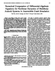
Example • J = (P1 − X2 , P22 − 1) ♦ • J is complete, but not quasi-linear. ♦ • J ` = (P1 − X2 ) ♦ • x = (x1 , x2 ) ∈ C2 implies ♦ π −1 (x) = { (x1 , x2 , x2, 1), (x1, x2 , x2 , −1) } • (π ` )−1 (x) = { (x1 , x2, x2 , p2 ) | p2 ∈ C } ♦ • W = W 0 = W ` = C2 and (W ` )0 = ∅. ♦ • rank J(x) = 1 for any x ∈ W 0 ♦ F. Leon Pritchard, York College; William Sit, City College,CUNY Algebraic Constraints on Initial Values of Differential Equations

Solutions to Example • System of ODEs: x˙ = y , y˙ 2 = 1 ♦ • Two solutions for each initial condition (x, y ) = (x0 , y0 ) ♦ x=±

t2 + y0 t + x0 , 2

y = ±t + y0 ,

3

2

1

-3

-2

1

-1

2

3

-1

-2

-3

F. Leon Pritchard, York College; William Sit, City College,CUNY Algebraic Constraints on Initial Values of Differential Equations

Theorem for Quasi-Linear Ideal Let J be a quasi-linear ideal in C[X, P]. There exist a computable non-negative integer ν, and ν non-empty, affine, effectively computable, Zariski basic open subsets U1 , . . . , Uν of the initial domain W of J with these properties: • W 0 = ∪νk=1 Uk ; in particular, W 0 is an effectively computable ♦ constructible subset of Cn . • For each k, 1 6 k 6 ν, the set Yk = π −1 (Uk ) is an affine, ♦ non-empty, Zariski basic open subset of the jet domain V of J. • For each k, 1 6 k 6 ν, the restriction πk of π to Yk is an ♦ isomorphism from Yk to Uk as affine sets. • For each k, 1 6 k 6 ν, the inverse isomorphism ♦ ηk : Uk −→ Yk is an everywhere defined rational map. • There is an unique isomorphism η : W 0 −→ π −1 (W 0 ) of affine ♦ schemes such that π(η(x)) = x for x ∈ W 0 . Morever, η|Uk = ηk for 1 6 k 6 ν. F. Leon Pritchard, York College; William Sit, City College,CUNY Algebraic Constraints on Initial Values of Differential Equations

Classical Existence and Uniqueness Theorem Let D be an open subset of Cn , and let the system v on D be ˙ given by z(t) = r(z(t)) for t ∈ R, where r : D −→ Cn is some analytic map. Then for any x0 ∈ D, there exist an interval B = (−, ) some  > 0, some open neighborhood O of x0 , and an analytic map ψ : B × O −→ D such that O ⊆ D, and for every x ∈ O, we have • ψ(0, x) = x ♦ • the map ψx : B −→ D defined by t 7→ ψ(t, x) is the unique ♦ solution defined on B satisfying the system v and the initial condition z(0) = x.

F. Leon Pritchard, York College; William Sit, City College,CUNY Algebraic Constraints on Initial Values of Differential Equations

Algebraic Setting • J be an ideal in C[X, P] ♦

• x ∈ Cn , B = (−, ) be an open interval in R ♦ • M be a constructible subset of Cn ♦

• A differentiable map ϕ : B −→ M is a differentiable map ♦ ϕ : B −→ Cn whose image is contained in M.

• A solution to the initial value problem (J, x) on B in M is a ♦ differentiable map ϕ : B −→ M such that ϕ(0) = x and f (ϕ(t), ϕ(t)) ˙ = 0 for all t ∈ B and for all f ∈ J. We also say: • ϕ satisfies the initial value problem (J, x) ♦ • (J, x) admits a solution in M ♦

• the image of ϕ is an integral curve of J through x. ♦ F. Leon Pritchard, York College; William Sit, City College,CUNY Algebraic Constraints on Initial Values of Differential Equations

Existence and Uniquenss Theorem I Let J be a complete quasi-linear ideal in C[X, P], let V and W be respectively the jet and initial domain of J, and let x0 ∈ W 0 . Then there exist some Euclidean open subset U of W 0 containing x0 , some interval B = (−, ) for some  > 0, and a mapping ϕ : B × U −→ W 0 , such that for every x ∈ U, we have • ϕ(0, x) = x; ♦ • the map ϕx (t) defined by t 7→ ϕ(t, x) is the unique solution ♦ on B in W 0 to the initial value problem (J, x); and • the map ϕ is the restriction of an analytic map ♦ ψ : B × O −→ Cn where O is a Euclidean open subset of Cn containing x0 such that U = W 0 ∩ O. F. Leon Pritchard, York College; William Sit, City College,CUNY Algebraic Constraints on Initial Values of Differential Equations

Sketch of Proof • ♦ • ♦ • ♦ • ♦ • ♦ • ♦

x0 ∈ W 0 implies for some n × n determinant det ∆(x0 ) 6= 0. Let f1 , . . . , fn define the matrix for ∆. ˙ On D = { x ∈ Cn | ∆(x) 6= 0 }, define v1 : z(t) = r(z(t)). Let q1 , . . . , q` generate J ∩ C[X]. P P Completeness implies ∆ · ∇qi = `i 0=1 hii 0 qi 0 + nj=1 qij fj . On D × C` define v2 :

˙ z(t) = r(z(t)), w˙ i (t) =

m X hii 0 (z(t)) i 0 =1

∆(z(t))

wi 0 (t) 1 6 i 6 `, t ∈ R.

• Let ϕ : B × U −→ D be a solution to v1 . ♦ • For any x ∈ U, (ϕ(t, x), 0) and ♦ (ϕ(t, x), q1 (ϕ(t, x)), . . . , q` (ϕ(t, x))) are solutions to v2 . • ϕ(t, x) ∈ W 0 . ♦ F. Leon Pritchard, York College; William Sit, City College,CUNY Algebraic Constraints on Initial Values of Differential Equations

Algorithm for the General Case • J an ideal in C[X, P] ♦ • Compute its completion ideal e ♦ J

• Compute a P-strong essential P-degree basis f1 , . . . , fm of the ♦ associated quasi-linear ideal e J ` of e J • Compute an irredundant representation U1 , . . . , Uν of ♦ f0 M0 = W

• For 1 6 k 6 ν, compute the vector field rk on Uk using ♦ Cramer’s Rule. • For any initial condition x0 , use any Uk containing x0 and ♦ integrate the vector field rk . F. Leon Pritchard, York College; William Sit, City College,CUNY Algebraic Constraints on Initial Values of Differential Equations

A Quasi-Linear Example Revisited • z1 (t), z2 (t), z3 (t) are functions of t ♦ • z˙1 (t), z˙2 (t), z˙3 (t) are their derivatives with respect to t ♦ −z2 z˙1 z3 z˙1

− z2 z˙2 + z1 z˙3 + 2z˙3 2 + z1 z˙2 − z1 z˙2 + z˙3

= z14 = 5z3 = 3z22 = z3

• Ideal version: J generated by polynomials ♦ −X2 P1 X3 P1

− X2 P2 + X1 P3 + 2P3 + X12 P2 − X1 P2 + P3

− X14 , − 5X3 , − 3X22 , − X3 .

F. Leon Pritchard, York College; William Sit, City College,CUNY Algebraic Constraints on Initial Values of Differential Equations

Illustration of Algorithm • J contains an algebraic constraint of total degree 7 in X. ♦ • The ideal has index 3. ♦ • an essential P-degree basis of the completion ideal is ♦ − −

X12 X1 X3 2X1 P1 X3 P1 X1 P2 X3 P2

+ X2 , + X22 , − P2 , − X22 , − 2X3 , − 2X2 X3 ,

− X1 X2 − X23 X2 P1 X2 P2 P3

+ X3 , + X32 , − X3 , − 2X22 , − 3X3 .

f 0 = { (x1 , x2, x3 ) ∈ C3 | x2 6= 0, x2 = x 2 , x3 = x 3 } • M0 = W ♦ 1 1 • an explicit system on M 0 is: ♦ P1 =

X3 , X2

P2 = 2X2 ,

P3 = 3X3 ,

X2 6= 0.

F. Leon Pritchard, York College; William Sit, City College,CUNY Algebraic Constraints on Initial Values of Differential Equations

Statistics

max deg in algebraic constraints max coefficient in constraints max P-degree in system

first second prolongation prolongation 36 10 95 digits 30 digits 4 4

F. Leon Pritchard, York College; William Sit, City College,CUNY Algebraic Constraints on Initial Values of Differential Equations

Non Quasi-Linear Example Revisited • x(t), y (t) functions of t ♦ • p(t), q(t) their derivatives with respect to t ♦ pq −yp + 3xq 4q 2 p2

= xy 2 = 3x + 6 = 9x 2 = x2 − 4

• The ideal J corresponding to this system is complete and has ♦ essential P-degree 2. F. Leon Pritchard, York College; William Sit, City College,CUNY Algebraic Constraints on Initial Values of Differential Equations

Illustration of the Algorithm • An essential P-degree basis gives another presentation: ♦ q2 27p + 6xyq 2 (4y + 54)q 0

= = = =

y 2 + 9, 4y 3 + 54y , 6xy 2 + 81x, 9x 2 − 4y 2 − 36.

• Retaining only the quasi-linear equations: rank (J, x) = 2 ♦ whenever 27(4y 2 + 54) 6= 0. • The explicit system is ♦ 2y 3x , q= . 3 2 • The integral curve v satisfying x(0) = x0 , y (0) = y0 is ♦ v:p=

2 x = x0 cosh(t) + y0 sinh(t), 3

3 y = y0 cosh(t) + x0 sinh(t). 2

F. Leon Pritchard, York College; William Sit, City College,CUNY Algebraic Constraints on Initial Values of Differential Equations

Comments on Example • This solution exists and lies on the hyperbola ♦ 9x 2 − 4y 2 − 36 = 0 whenever (x0 , y0 ) does. • The solution satisfies q 2 (t) = y 2 (t) + 9 for all t. ♦ • When 2y02 + 27 = 0, we have x02 + 2 = 0. ♦ p √ • The four points (± −2, ±3 −3/2) are equilibrium solutions ♦ J `. • They are not solutions to J, nor are equilibrium points of v. ♦ • At these 4 initial conditions, (J ` , x) does not have uniqueness ♦ solutions, but (J, x) does. • The sets of solutions for J ` and J are not the same. ♦ F. Leon Pritchard, York College; William Sit, City College,CUNY Algebraic Constraints on Initial Values of Differential Equations

Existence and Uniqueness Theorem II Let J = (g1 , . . . , gm ) be an ideal in C[X, P], and consider the system of differential algebraic equations g1 (z1 , . . . , zn , z˙1 , . . . , z˙n ) = 0, .. . gm (z1 , . . . , zn , z˙1 , . . . , z˙n ) = 0. Then we can effectively compute • (1) a Zariski-closed subset M of Cn and some integer ν > 0; ♦ • (2) for each k, 1 6 k 6 ν, a non-empty Zariski open subset ♦ Uk of M; • (3) for each k, 1 6 k 6 ν, an n-dimensional vector ♦ rk = (rk,1 , . . . , rk,n ) of rational functions in C(X)n , everywhere defined on Uk such that F. Leon Pritchard, York College; William Sit, City College,CUNY Algebraic Constraints on Initial Values of Differential Equations

• (4) the union M 0 = ∪νk=1 Uk is irredundant; ♦ • (5) for every  > 0 and for every x ∈ M 0 , the image of a ♦ differentiable map ψx : B −→ M 0 is an integral curve of J through x if and only if ψx (0) = x and for every k, 1 6 k 6 ν, such that x ∈ Uk , we have ψ˙ x (t) = rk (ψx (t)); • (6) for every x0 ∈ M 0 , there exist some  > 0, some open ♦ neighborhood U of x0 in M 0 and a map ϕ : B × U −→ M 0 such that for every x ∈ U, the image of the map ϕx : B −→ M 0 defined by t 7→ ϕ(t, x) is an integral curve of J through x; and • (7) for any x ∈ ♦ / M, the initial value problem (J, x) does not admit a solution on B in Cn for any  > 0. F. Leon Pritchard, York College; William Sit, City College,CUNY Algebraic Constraints on Initial Values of Differential Equations

Algorithm for Explicit Form • Input: (1) An essential P-degree basis f1 , . . . , fm for a ♦ complete quasi-linear ideal J in C[X, P], or in matrix form L:

A(X)PT = c(X)

• (2) Polynomials q1 , . . . , q` generating J ∩ C[X] (defining W ) ♦ • Output: An irredundant representation of W 0 = ∪νk=1 Uk and ♦ for each Uk , a vector of rational functions rk (X) for the vector ˙ field v : z(t) = rk (z(t)) • May use in (1) only those fi which has P-degree 1, and in (2) ♦ those fi which has P-degree 0. • Each Uk will be given by defining equations and inequations. ♦ F. Leon Pritchard, York College; William Sit, City College,CUNY Algebraic Constraints on Initial Values of Differential Equations

Subroutines Adapted from Sit’s (1992) algorithm for parametric linear equations. • Determinants(A(X)) returns the set ∆ of all non-zero ♦ determinants of n × n submatrices of A(X) if none of these determinants are constants; otherwise, it returns {∆} where ∆ is one such non-zero, constant determinant. We assume that any determinant returned by this routine carries with it the row index set a. • MinGenerator(h), where h = (h1 , . . . , hs ) is a family of ♦ polynomials. This procedure returns a minimal subfamily H = (hi1 , . . . , hik ) of h such that for every j, 1 6 j 6 s, hj belongs to the radical of (H). • Solve(L, a) returns the unique solution vector ra (X) of ♦ rational functions in C(X) to the linear system Aa (X)PT = c a (X). F. Leon Pritchard, York College; William Sit, City College,CUNY Algebraic Constraints on Initial Values of Differential Equations

Algorithm for Explicit Form begin S ←− ∅ if m < n then return W 0 = ∅ else h ←− Determinants(A(X)) H ←− MinGenerator(h) for ∆a ∈ H do Da ←− { x ∈ Cn | ∆a (x) 6= 0 } Ua ←− Da ∩ W ra ←− Solve(L(X), a) S ←− S ∪ { a } end return { (Ua , ra ) | a ∈ S } end F. Leon Pritchard, York College; William Sit, City College,CUNY Algebraic Constraints on Initial Values of Differential Equations

Axiom Implementation • [makeSytem(F ):] creates internal representation S for the ♦ ideal J given by polynomials F = { f1, . . . , fm } ⊂ Q[X]

• [matrixView(S):] displays system S in matrix form if the ideal ♦ represented by S is quasi-linear. • [algebraicSystem(S):] displays a generating set of polynomials ♦ in J ∩ Q[X], when the ideal J has representation S.

• [linearize(S):] computes a system S ` representing the ♦ associated linear ideal J ` of the ideal J, where J is represented by the system S. • [prolong(S):] computes the system S ∗ representing the ♦ prolongation J ∗ of the ideal J where J is represented by S. • [complete?(S):] returns true if the ideal J represented by S is ♦ complete, and false otherwise. F. Leon Pritchard, York College; William Sit, City College,CUNY Algebraic Constraints on Initial Values of Differential Equations

e for the • [completion(S):] computes the representation S ♦ completion e J of J, when J is represented by S.

• [index(S):] computes index of J, when J is represented by S. ♦ • [parSolve(S):] computes the algebraic conditions for the ♦ matrix A(X) associated with a quasi-linear ideal J represented by S to have rank n and computes the rational functions ri (X) which represent coordinates of P such that when x ∈ W and satisfies the algebraic conditions, p = (r1 (x), . . . , rn (x)) satisfies the linear system A(X) = c(X). Adapted from the ParametricLinearEquations package. • The data structure S allows caching of all prolongation and ♦ completion computations. Routines that cache results: prolong, index, complete? and completion. • An essential P-degree basis is kept for all ideals. ♦ F. Leon Pritchard, York College; William Sit, City College,CUNY Algebraic Constraints on Initial Values of Differential Equations

Unconstrained and Underdetermined Ideals • J an ideal in C[X, P] ♦ • J is unconstrained if J ∩ C[X] = (0). ♦ • unconstrained implies complete ♦ f ` )0 = ∅ • J is underdetermined if (W ♦

• Intuitively, underdetermined means there is no initial ♦ conditions x0 that will guarantee a unique solution. Either some dependent variable will be arbitrary, or there are multiple integral curves through x0 . • These properties are algorithmically decidable. ♦ F. Leon Pritchard, York College; William Sit, City College,CUNY Algebraic Constraints on Initial Values of Differential Equations

Example of Underdetermined Ideal • J = (X1 X2 − 1, P12 − X12 , P22 − X22 ) ♦

• Index 1 with e J = (P12 − X12 , P2 + X22 P1 , X1 X2 − 1), ♦ f is the hyperbola X1 X2 = 1. • W ♦

f. • rank e ♦ J ` (x) = 1 for any x ∈ W

f` 0 = ∅. • J is underdetermined, W ♦

• z = (ϕ1 , ϕ2 ), ϕ2 arbitrary, ϕ2 (t) 6= 0 for all t, and ϕ1 = 1/ϕ2 . ♦ • Differential algebraic system: z1 z2 = 1, z˙12 = z12 , z˙22 = z22 ♦ • Initial conditions z(0) = (x1 , x2 ) where x1 x2 = 1 ♦ • Two solutions (x1 e ±t , x2 e ∓t ) ♦ F. Leon Pritchard, York College; William Sit, City College,CUNY Algebraic Constraints on Initial Values of Differential Equations

Quasi-linearization of Ideals • J be an ideal in C[X, P]. ♦

• Y = (Y1 , · · · , Y2n ) and Q = (Q1 , · · · , Q2n ) indeterminates ♦ • λ : C[X, P] −→ C[Y] where λ(g ) = g (Y1 , · · · , Y2n ) ♦

• Quasi-linearization of J is the ideal in C[Y, Q] given by ♦ q`(J) = ({ Qk − Yn+k | 1 6 k 6 n } ∪ { λ(g ) | g ∈ J }) • J = (g1 , . . . , gm ) implies ♦ { Qk − Yn+k | 1 6 k 6 n } ∪ { λ(gi ) | 1 6 i 6 m } is a Q-strong essential Q-degree basis for q`(J). • q`(J ∗ ) ⊆ q`(J)∗ . ♦ F. Leon Pritchard, York College; William Sit, City College,CUNY Algebraic Constraints on Initial Values of Differential Equations

Quasi-linearization Helps • J = (X1 X2 − 1, P12 − X12 , P22 − X22 ) (underdetermined ex.) ♦

• q`(J) = (Q1 − Y3 , Q2 − Y4 , Y1 Y2 − 1, Y32 − Y12 , Y42 − Y22 ) ♦ ] = (Q4 − Y2 , Q3 − Y1 , Q2 + Y3 Y 2 , Q1 − Y3 , • q`(J) ♦ 2 Y1 Y2 − 1, Y4 + Y3 Y22 , Y32 − Y12 ) ^) : Y1 Y2 − 1 = 0, • q`(W ♦

Y4 + Y3 Y22 = 0,

] ^) • rank q`(J)(y) = 4 for any y ∈ q`(W ♦ • Translation: ♦

Y32 − Y12 = 0

Y1 Y2 Y3 Y4 Q1 Q2 Q3 Q4 z1 z2 z˙1 z˙2 z˙1 z˙2 z¨1 z¨2

• Second Order System: z¨1 = z1 , ♦ • Constraints: z1 z2 = 1, ♦

z˙12 = z12 ,

z¨2 = z2 z¨2 = −z˙1 z22

• It is necessary to decide the branch by giving z˙ 1 (0) only. ♦ F. Leon Pritchard, York College; William Sit, City College,CUNY Algebraic Constraints on Initial Values of Differential Equations

Underdetermined Quasi-Linear Example • System: ♦ (−x + y )x˙ + x y˙ + (x 2 − 1)z˙ = 0 2 y x˙ + (x + 1)y˙ + x 3 z˙ = 0 • Solutions: Every constant point is an equilibrium solution. ♦ • Complete System (Index 0) ♦ • Explicit System: No algebraic constraints. k arbitrary. ♦ x˙ = k y˙ = k(x 4 − (x 3 + x 2 − 1)y ) z˙ = k(−x 3 − x + (x 2 − x + 1)y ) • We can obtain unique solution by adding any quasi-linear ♦ equation g (X, P) = 0, for example x˙ = 1. F. Leon Pritchard, York College; William Sit, City College,CUNY Algebraic Constraints on Initial Values of Differential Equations

Underdetermined Quasi-linear Systems • J complete, quasi-linear ideal, underdetermined ♦ • Assume W is irreducible. ♦ • ρ = max{ rank J(x) | x ∈ W } < n ♦ • g1 , . . . , gν (ν 6 n − ρ) polynomials of P-degree 1 ♦ • J1 = (J, g1 , . . . gν ) ♦ • Suppose W1 contains a point x0 with rank J1 (x0 ) = ρ + ν. ♦ • Then J1 ∩ C[X] = J ∩ C[X]. ♦ F. Leon Pritchard, York College; William Sit, City College,CUNY Algebraic Constraints on Initial Values of Differential Equations

Primary Decomposition

• J complete, but not necessarily quasi-linear ♦ • R(J) = ♦

p J ∩ C[X]

• R = Q1 ∩ · · · ∩ Qr : irredundant primary (prime) decomposition ♦ • Ki = (J ∪ Qi ∪ ∇Qi ) ♦ • J quasi-linear implies Ki quasi-linear ♦ • J complete implies Ki complete and Ki ∩ C[X] = Qi . ♦ F. Leon Pritchard, York College; William Sit, City College,CUNY Algebraic Constraints on Initial Values of Differential Equations

Conclusions • Approach is ideal theoretic, providing maximum flexibility in ♦ implementation • Applies to all eventually quasi-linear systems without any ♦ transformation • Applies to overdetermined as well as underdetermined systems ♦ • Applies to non-linear systems either by a transformation or by ♦ dropping some non-linear equations • Any system may be completed with no a priori conditions. ♦

• Existence and Uniqueness theorem holds for computed initial ♦ conditions • Provides equivalent explicit form ready for numerical methods ♦ and dynamical analysis F. Leon Pritchard, York College; William Sit, City College,CUNY Algebraic Constraints on Initial Values of Differential Equations

• Campbell, S. L. (1980). Singular Systems of DIfferential ♦ Equations. Research Notes in Mathematics, 40. Pitman, New York. • Campbell, S. L. (1985). The Numerical Solution of Higher ♦ Index Linear Time Varying Singular Systems of Differential Equations. Siam. J. Sci. Stat. Comput., 6, 334–348. • Campbell, S. L. (1987). A General Form for Solvable Linear ♦ Time Varying Singular Systems of Differential Equations. Siam. J. Math. Anal., 18, 1101–1115. • Campbell, S. L. and Griepentrog, E. (1995). Solvability of ♦ General Differential Equations. Siam. J. Sci. Comp., 16(2), 257–270. • Gear, C. W. (1988). Differential-Algebraic Equation Index ♦ Transformations. Siam. J. Sci. Stat. Comput., 9(1), 39–47. F. Leon Pritchard, York College; William Sit, City College,CUNY Algebraic Constraints on Initial Values of Differential Equations

• Gear, C. W. and Petzold, L. R. (1983). Differential/Algebraic ♦ Systems and Matrix Pencils. Matrix Pencils (eds. B. Kagstrom and A. Ruhe), Lecture Notes in Math., 973, 75–89, Springer-Verlag. • Gear, C. W. and Petzold, L. R. (1984). ODE Methods for the ♦ Solution of Differential/Algebraic Systems. SIAM J. Numer. Anal. 21, 367–384. • Kunkel, P. and Mehrmann, V. (1994). Canonical Forms for ♦ Linear Differential-Algebraic Equations with Variable Coefficients. J. Comput. Appl. Math., 56, 225–251. • Kunkel, P. and Mehrmann, V. (1996a). A New Class of ♦ Discretization Methods for the Solution of Linear Differential-Algebraic Equations with Variable Coefficients. SIAM J. Numer. Anal., 33(5), 1941–1961. F. Leon Pritchard, York College; William Sit, City College,CUNY Algebraic Constraints on Initial Values of Differential Equations

• Kunkel, P. and Mehrmann, V. (1996b). Local and Global ♦ Invariants of Linear Differential-Algebraic Equations and Their Relation. Electronic Trans. Num. Anal., 4, 138–157. • Rabier, P. J., Rheinboldt, W. C. (1991). A General Existence ♦ and Uniqueness Theory for Implicit Differential-Algebraic Equations. Differential Integral Equations, 4, 563–582. • Rabier, P. J., Rheinboldt, W. C. (1994). A Geometric ♦ Treatment of Implicit Differential-Algebraic Equations. J. of Differential Equations, 109, 110–146. • Reich, S. (1988). Differential-Algebraic Equations and Vector ♦ Field on Manifolds. Sekt. Informationstechnik, Nr. 09-02-88, T.U. Dresden. • Reich, S. (1989). Beitrag zur Theorie der ♦ Algebrodifferentialgleichungen. Ph. D. Dissertaion in Engineering, T.U. Dresden. F. Leon Pritchard, York College; William Sit, City College,CUNY Algebraic Constraints on Initial Values of Differential Equations

• Sit, W. Y. (1992). An Algorithm for Solving Parametric Linear ♦ Systems. J. Symbolic Computation, 13, 353–294. • Thomas, G. (1996). Symbolic Computation of the Index of ♦ Quasi-linear Differential-Algebraic Equations. Proc. ISSAC’96, Lakshman, Y.N. ed., 196–203. ACM Press. • Tuomela, J. (1997). On the Resolution of Singularities of ♦ Ordinary Differential Systems. Research Report A388, Helsinki University of Technology.

F. Leon Pritchard, York College; William Sit, City College,CUNY Algebraic Constraints on Initial Values of Differential Equations