Page 1 ... The main advantage of using such methods is that we can optimize systems consisting of multiple .... the well known compiler optimization techniques.
Journal of VLSI Signal Processing 49, 31–50, 2007
* 2007 Springer Science + Business Media, LLC. Manufactured in The United States. DOI: 10.1007/s11265-007-0137-7
Algebraic Methods for Optimizing Constant Multiplications in Linear Systems ANUP HOSANGADI Synthesis Group, Cadence Design Systems, San Jose, CA 95134, USA FARZAN FALLAH Advanced CAD Technology, Fujitsu Laboratories of America, Sunnyvale, CA 94085, USA RYAN KASTNER Department of Electrical and Computer Engineering, University of California, Santa Barbara, Santa Barbara, CA 93106, USA Received: 4 March 2005; Revised: 2 February 2006; Accepted: 23 October 2006
Abstract. Constant multiplications can be efficiently implemented in hardware by converting them into a sequence of nested additions and shift operations. They can be optimized further by finding common subexpressions among these operations. In this work, we present algebraic methods for eliminating common subexpressions. Algebraic techniques are established in multi-level logic synthesis for the minimization of the number of literals and hence gates to implement Boolean logic. In this work we use the concepts of two of these methods, namely rectangle covering and fast extract (FX) and adapt them to the problem of optimizing linear arithmetic expressions. The main advantage of using such methods is that we can optimize systems consisting of multiple variables, which is not possible using the conventional optimization techniques. Our optimizations are aimed at reducing the area and power consumption of the hardware, and experimental results show up to 30.3% improvement in the number of operations over conventional techniques. Synthesis and simulation results show up to 30% area reduction and up to 27% power reduction. We also modified our algorithm to perform delay aware optimization, where we perform common subexpression elimination such that the delay is not exceeded beyond a particular value. Keywords: algebraic methods, constant multiplications, linear systems, DSP synthesis, high level synthesis, common subexpression elimination 1.
Introduction
Most of the present generation embedded systems, such as cellular phones, video cameras and handhelds perform some kind of continuous numeric processing on input data. The frequent use of these computation intensive kernels and the large parallelism available in these computations make them amenable to hardware implementations. In most
cases the performance and power consumption of the whole system is directly dependant on these computations. Since embedded systems are increasingly becoming complex, it is important to develop automated techniques that can optimize these computations. Reducing the number of operations by redundancy elimination techniques is a good way to improve performance and reduce power consumption. This article presents a novel technique for
32
Hosangadi et al.
reducing the number of computations in a set of linear arithmetic expressions implemented in application specific integrated circuits (ASICs). Linear arithmetic computations can be found in a number of applications, mainly in communications, control and signal processing. When the constant multiplications need to be implemented in hardware, the full flexibility of a multiplier is not necessary, and the multiplication can be implemented as a sequence of additions and hardwired shift operations. The relative cost of adder and multiplier depends on the adder and multiplier architectures in addition to the implementation technology. For example, a k�k array multiplier has twice the latency and k times the area of a k-bit ripple carry adder. For example consider the integer multiplication 7�X as shown in Fig. 1. Using two_s complement representation for the constants, it is possible to implement this multiplication using two additions and two shift operations. Using signed digit representations reduces the number of non-zero digits in the representation of the constant, which reduces the number of additions. Figure 1 shows that by using the canonical signed digit (CSD) representation it is possible to implement 7�X using only one addition and one shift operation. The number of operations can be further reduced by finding common subexpressions among the set of constant multiplications. Conventional methods find common subexpressions among the set of constants multiplying a single variable, by looking at common digit patterns in the constants involved. For example, in the operations 7�X and 13�X shown in Fig. 2, the common digit pattern B101^ can be observed in the two constants B7^ and B13^. This common digit pattern corresponds to the common subexpression BX+X¡2^. Eliminating this common subexpression reduces the number of additions by one, as shown in Fig. 2. Most of the earlier works for finding common subexpressions in systems involving constant multiplications were based on finding common digit
Figure 1. additions.
Converting constant multiplications into shifts and
Figure 2. Eliminating common subexpressions by finding common digit patterns.
patterns in the set of constants multiplying a single variable [1–9]. These methods are good enough for optimizing systems where only single variable optimizations are required, such as the transformed form of FIR digital filters. But such methods do not do a good optimization of systems consisting of multiple variables. Many operations in DSP can be expressed in the form of a multiplication of a constant matrix with a vector of input samples X of the form shown in Eq. (1) , where ci,j represents the (i,j)th element in an N�N constant matrix. Y ½i� ¼
N �1 X
ci;j � X½ j�
ð1Þ
j¼0
Just performing optimizations for a single variable at a time is not sufficient to do a good optimization for these systems. As an illustration consider the example linear system, consisting of the variables X1 and X2, shown in Fig. 3a. Looking at common digit patterns in the constants multiplying variable X2 (7=B0111^ and 12=B1100^) the common digit pattern B11^ is detected and the number of operations can be reduced by one, as shown in Fig. 3c. But by eliminating common subexpressions to include multiple variables, it is possible to further reduce the number of additions by two as shown in Fig. 3d. To the best of our knowledge such an optimization cannot be done by any of the known techniques. In this paper we present algebraic techniques that can perform the kind of optimizations shown in Fig. 3d. The rest of the paper is organized as follows. Section 2 presents and compares related work in optimizing linear computations. We formulate the problem to be solved and introduce our polynomial transformation of linear systems in Section 3.
Algebraic Methods for Optimizing Constant Multiplications
Figure 3.
Example showing the improvement obtained by extending common subexpressions involving multiple variables.
Section 4 presents a technique for eliminating common subexpressions using a rectangle covering approach. Section 5 presents an improved technique for eliminating common subexpressions by iteratively eliminating two-term common subexpressions. We also present here a delay aware subexpression elimination algorithm. We present experimental results on a set of commonly used DSP transforms in Section 6, where we compare the reduction in the number of operations and its effect on the performance, area and power consumption of the synthe-
Figure 4.
33
Coefficient transformation using matrix splitting.
sized examples. Finally we conclude the paper in Section 7. 2.
Related Work
Common subexpression elimination (CSE) is one of the well known compiler optimization techniques and is applied at both the local as well as the global scopes of the program. [10]. In addition to CSE, modern optimizing compilers also perform Value numbering [11] and strength reduction [12]. Value
34
Hosangadi et al.
numbering assigns numbers to variables in the program and detects equality among variables if they have the same values throughout the execution of the program. In addition it discovers constant values, evaluates expressions with constant operands and propagates them through the code. Strength reduction is useful in many cases such as address calculation, where expensive multiplications can be reduced to additions. CSE and Value numbering are powerful transformations for general purpose applications, but they fail to perform the best optimizations for arithmetic expressions, as they do not take advantage of the associative and distributive properties of arithmetic operators. The work in [13] exploited these properties targeted at exposing more loop invariant operations, but even this method does not guarantee that all possible common subexpressions would be detected, which our methods described in this paper do. Recent works have shown that vast improvement in performance and power consumption can be achieved by using more sophisticated optimization techniques [14–19]. Our methods have been designed only for arithmetic operations and can be used in blocks without any control flow. The traditional compiler techniques discussed previously [11–13] are more general in the sense that they can be applied at both the local and global scopes of the program. Extending our methods to perform optimizations globally could result in a more practical and powerful technique. In this paper, we target our optimizations for hardware synthesis, and we compare our results with those produced by hardware centric approaches, where we observe tremendous improvements in area and power consumption. The problem of reducing the number of operations by decomposing constant multiplications into shifts and additions has been studied for a long time [20, 21]. This early work led to the invention of a novel number representation scheme called the canonical signed digit (CSD) [22]. The CSD representation, on an average reduces the number of nonzero digits in a constant representation by 33% compared to the conventional two_s complement representation. This leads to a direct reduction in the number of addition operations. CSD multipliers have been used for low complexity FIR filter design [9]. There have been a number of works on optimizing constant multiplications in FIR filter design by efficient encoding of coefficients and sharing of common computations [1, 5, 23].
The first work that addressed the different issues and suggested solutions to the multiple constant multiplication (MCM) problem, was in [3]. This work used an iterative bipartite matching algorithm, where in each iteration the best two matching constants were selected and the matching parts eliminated. This bipartite matching algorithm was combined by a preprocessing scaling of the input constants for an increased solution space. Though scaling of the coefficients is an effective technique for reducing the number of operations, the exponential search space for finding the right scaling factor does not make it a practical approach for solving the problem. A drawback of the proposed algorithm is that the bipartite matching algorithm is not the best approach for eliminating common subexpressions, and a more global approach is required. Furthermore, this algorithm cannot find common subexpressions among shifted forms of the constants. For example, it cannot detect the common subexpression B101^ between the constants B0101^ and B1010^. The works in [2, 24, 25] perform a greedy optimization procedure to minimize the area of linear digital systems using combination of techniques modifying the coefficient matrices and common subexpression elimination. The modification of the coefficients is based on the fact that the complexity of the multiplier is dependant on the value of the coefficient and transforms the linear system by splitting the constant matrices such that the overall area is reduced. The matrix decomposition technique splits a system matrix M into the product of (2z+1) matrices M=MzMzj1Mzj2... M0...Mjz+1Mjz. The matrix splitting is obtained by row and column transformations. Figure 4 shows an example of matrix splitting used in a linear system, used in [2]. This matrix splitting was combined with shift-and-add decomposition of constant multiplications and an algorithm to eliminate common subexpressions in [2]. The algorithm was based on bipartite matching, similar to [3], but was extended to find common subexpressions among shifted forms of the constants. For example, it could detect the common pattern B101^ among the patterns B1010^ and B0101^. A major disadvantage of this method is that it cannot find common subexpressions involving multiple variables, which leads to inferior solutions, as we show in our experimental results. Our method does not consider the modifications of the coefficient matrices, since it is a method that only eliminates
Algebraic Methods for Optimizing Constant Multiplications
common subexpressions. It assumes that a coefficient matrix is already given. There have been plenty of methods for eliminating common subexpressions based on the digit pattern matching techniques, particularly for the optimization of FIR digital filters. For the transposed form of FIR filters (shown in Fig. 5), it is sufficient to optimize multiplications involving a single variable. The idea of replacing the multipliers with a computation sharing multiplier block was first introduced in [26], where the sharing was obtained by finding common digit patterns among the set of coefficients. Graph theoretic approaches have been used to synthesize the multiplier block by finding minimal differences among the coefficients [6, 7, 27], where the nodes in the graph denote the coefficients and the edges denote the differences between the coefficients. Exhaustive pattern generation and matching techniques have also been explored in [1], where all possible patterns having two or more non-zero digits are generated and a matching is performed among them. Though these methods produce good results for FIR filters, they do not do a good optimization for multiple variable systems. Our methods can find all the common subexpressions detected by these methods in addition to finding common subexpressions involving multiple variables. The final reduction in the number of operations produced by any optimization algorithm depends on
Figure 5.
Structures for FIR digital filters.
35
the initial representation of the constants. Although using CSD representation of the constants produces the least number of operations before optimization, it does not imply the least number of operations after eliminating common subexpressions. The best results can be obtained by using a mixed representation of the coefficients involved, as observed in [5]. But the exponential number of combinations that need to be considered does not make it practical to use such an approach. In our work, we use only a single representation, namely CSD for the constants. The main optimization in multi-level logic synthesis is the reduction of the number of literals in a set of Boolean functions by performing decomposition and factoring. These functions typically contain hundreds of variables and thousands of literals and therefore various efficient techniques have been developed to handle the large complexity [28]. Performing Boolean decomposition and factoring for large instances is computationally infeasible [29], and simplified procedures such as algebraic decomposition and factoring are generally preferred. Decomposition is the process of pulling out common subexpressions consisting of two or more cubes (terms) until there are no more common subexpressions to be found. Figure 6 shows the decomposition of the Boolean functions F, G and H, by extracting the common factors X=(a+b) and Y=cd. We have adapted the techniques for algebraic decomposition
36
Hosangadi et al.
Figure 6.
Polynomial representation of example linear system.
The main contribution of our work is an algorithm that can optimize a system consisting of any number of variables. We now introduce our polynomial transformation which enables us to perform such an optimization. 3.1. Polynomial Transformation of Constant Multiplications
for Boolean expressions [30, 31] to the problem of finding and eliminating common subexpressions in linear arithmetic expressions. The key modifications include the novel polynomial transformation for constant multiplications to handle the shift operator and the algorithms for finding kernels for the method using rectangle covering (Section 4) and the algorithm for finding two-term divisors (Section 5). Furthermore, we need to consider the overlapping of terms for linear expressions, when eliminating common subexpressions (Section 4 and Section 5). 3.
Problem Formulation and Polynomial Transformation
The problem to be solved can be formulated as thus: Given a system of linear arithmetic expressions consisting of additions/subtractions and the multiplications are only with constant operands, assume that all the constant multiplications are to be decomposed into additions/subtractions and shift operations. Also assume that there are an infinite number of resources (ALUs and routing resources) that are available to implement the system. In such a scenario, reducing the number of additions that have to be implemented has a direct impact on the area. The dynamic power consumption is roughly proportional to the number of operations per unit of time, and the leakage power consumption also increases with the increase in the number of transistors. The objective is to reduce the number of additions/ subtractions as much as possible which would result in lower area and lower total power consumption. We also present a variation of our algorithm, where we reduce the number of additions/subtractions without increasing the length of the critical path. An optimal solution to the common subexpression elimination problem has been recently formulated [32] using 0–1 integer linear programming (ILP). But the formulation is only for single variable systems such as those found in FIR filters. Most of the other works in this area have the same limitation.
This polynomial transformation helps us to find common subexpressions involving any number of variables. Using a given representation of the integer constant C, the multiplication with the variable X can be represented as C�X ¼
X � � � XLi i
where L represents the left shift from the least significant digit and the i_s represent the digit positions of the non-zero digits of the constant, 0 being the digit position of the least significant digit. Each term in the polynomial can be positive or negative depending on the sign of the non-zero digit. Thus this representation can handle signed digit representations such as the canonical signed digit (CSD). For example the constant multiplication (12)decimal� X=(1100)binary�X=XL2+XL3 in our polynomial representation. In case of systems where the constants are
Figure 7.
Algorithm for generation of kernels.
Algebraic Methods for Optimizing Constant Multiplications
real numbers represented in fixed point, the constant can be converted into an integer, and the final result can be corrected by shifting right. For example in the constant multiplication (0.101)binary�X=(101)binary� X�2j3=(X+XL2)�2j3 in our polynomial representation. The linear system in Fig. 3a and b can be written using our polynomial formulation as shown in Fig. 7. The subscripts in parenthesis represent the term numbers which will be used in our optimization algorithm. 4.
Optimization Using Rectangle Covering
This section presents a technique to find common subexpressions by transforming the problem as a rectangle covering problem. First, a set of all algebraic divisors of the polynomial expressions is generated and arranged in a matrix form, from which all possible common subexpressions, involving any number of variables can be detected. A heuristic rectangle covering algorithm is then used to iteratively find common subexpressions. 4.1. Generating Kernels of Polynomial Expressions A kernel of a polynomial expression is a subexpression that is derived from the original expression through division by an exponent of L, and contains at least one term with a zero exponent of L, and all the terms of the original expression that had higher exponents of L. A divisor of a polynomial expression is a subexpression of the expression having at least one term with a zero exponent of L. The set of kernels of a polynomial expression is a subset of the set of divisors of the expression. The algorithm for generating kernels of a set of polynomial expressions is shown in Fig. 8. The algorithm recursively finds kernels within kernels generated by dividing by the smallest exponent of L. The exponent of L that is used to divide the original expression to obtain the kernel is the corresponding co-kernel of the kernel expression.
Figure 8.
Set of kernels and co-kernels for expressions in Fig. 6.
Figure 9.
37
Overlap between kernel expressions.
For example consider the expression Y1 in Fig. 7. Since Y1 satisfies the definition of a kernel, we record Y1 as a kernel with co-kernel F1_. The minimum nonzero exponent of L in Y1 is L. Dividing by L we obtain the kernel expression X1L+X2+X2L, which we record as a kernel with co-kernel L. This expression has L as the minimum non-zero exponent of L. Dividing by L, we obtain the kernel X1+X2 with cokernel L2. No more kernels are generated and the algorithm terminates. For expression Y2 we obtain the kernel X1+X2+X2L with co-kernel L2. The set of kernels and co-kernels for the expressions in Fig. 7 are shown in Fig. 9. The importance of kernels is illustrated by the following theorem. Theorem There exists a k-term common subexpression if and only if there is a k-term non-overlapping intersection between at least two kernels.
This theorem basically states that each common subexpression in the set of expressions appears as a non-overlapping intersection among the set of kernels of the polynomial expressions. Here a nonoverlapping intersection implies that the set of terms involved in the intersection are all distinct. As an example of overlapping terms, consider the binary constant B1001001^ represented in Fig. 10. Converting the multiplication of this constant with the variable X into our polynomial representation, we get the expression (1)X+(2)XL3+(3)XL6. There are two kernels generated: X+XL3+XL6 covering terms 1, 2 and 3 and X+XL3, covering terms 2 and 3. An intersection between these two kernels will detect two instances of the subexpression X+XL3, but they overlap as they both cover term 2. This overlap can wbe seen in the overlap between the two instances of the bit-pattern B1001^ as seen in Fig. 10. Implementing the polynomial X+XL3+XL6 with two instances of X+XL3 will result in the second term XL3 being covered twice. Though we can still implement it this way, and subtract XL3 at the end,
38
Hosangadi et al.
as above, this common subexpression will be detected by an intersection among the set of kernels. 4.2. Matrix Transformation to Find Kernel Intersections Figure 10.
Kernel Intersection Matrix (KIM).
it will not be beneficial in this case, as it would result in more additions than the original polynomial representation. Proof If: If there is a k-term non-overlapping intersection among the set of kernels, then it means there is a multiple occurrence of the k-term subexpression in the set of polynomial expressions, and the terms involved in the intersection are all distinct. Therefore a k-term non-overlapping intersection in the set of kernels implies a k-term common subexpression. Only If: Assume there are two instances of the k-term common subexpression. First assume the common subexpression satisfies the definition of a divisor, which means there is at least one term with a nonzero exponent of L. Now each instance of the subexpression will be a part of some kernel expression. This is because from the kernel generation algorithm (Fig. 8), each kernel is generated recursively dividing through the lowest (non-zero) exponent of L. Each time a division by L is performed all terms that already had a zero exponent of L will be discarded and other terms will be retained. The exponents of L in all the remaining terms will then be reduced by the lowest exponent of L. Each kernel expression contains all possible terms with zero exponent of L at that step, as well as all terms with higher exponents of L. Therefore if an instance of the common subexpression belongs to a polynomial, it will be a part of one of the kernel expressions of the polynomial. Both instances of the common subexpression will be a part of some kernel expressions and an intersection in the set of kernels will detect the common subexpression. If the common subexpression does not satisfy the definition of a divisor, which means it does not have any term having a zero exponent of L, the subexpression obtained through division by the smallest exponent of L will also be a common subexpression, and will satisfy the definition of a divisor. Reasoning
The set of kernels generated is transformed into a matrix form called the kernel intersection matrix (KIM), to find kernel intersections. There is one row for each kernel generated and one column for each distinct term in the set of kernel expressions. Each term is distinguished by its sign (+/j), variable and the exponent of L. Figure 11 shows the KIM for our example linear system from its set of kernels and cokernels shown in Fig 9. The rows are marked with the co-kernels of the kernels which they represent. Each F1_ element (i,j) in the matrix represents a term in the original set of expressions which can be obtained by multiplying the co-kernel in row i with the kernel term in column j. The number in parenthesis represents the term number that the element represents. Each kernel intersection appears in the matrix as a rectangle. A rectangle is defined as a set of rows and columns such that all the elements are F1_. For example in the matrix in Fig 11, the row set {1,4} and the column set {1,3,4} together make a rectangle. A prime rectangle is defined as a rectangle that is not contained in any other rectangle. The value of a rectangle is defined as the number of additions saved by selecting that rectangle (kernel intersection) as a common subexpression and is given by ValueðR; CÞ ¼ ðR � 1Þ � ðC � 1Þ
ð2Þ
where R is the number of rows and C is the number of columns of the rectangle. The value of the rectangle is calculated after removing the appropriate rows and columns to remove overlapping terms and obtain a maximal irredundant rectangle (MIR). We need to find the best set of common subexpressions (rectangles) such that the number of additions/ subtractions is a minimum. A similar problem is encountered in multi-level logic synthesis [28, 30], where the least number of literals in a set of Boolean expressions is obtained by a minimum weighted rectangular covering of the matrix, which is NP hard [33]. Our problem is different since we have to deal with overlapping rectangles in our matrix. We use a
Algebraic Methods for Optimizing Constant Multiplications
Figure 11.
39
Algorithm for finding kernel intersections.
greedy algorithm, where in each iteration, we pick the best non-overlapping prime rectangle. Picking only non-overlapping prime rectangles need not always give the best results, since sometimes it may be beneficial to select a rectangle with overlapping terms and then subtract the terms that are covered more than once. We would like to consider the effect of selecting overlapping rectangles and observe its effect on the quality of the result in the future. Worst case analysis of KIM In the worst case, we have every possible term forming the columns in the KIM, and every possible exponent of L for each expression forming the rows. Consider an m�m constant matrix with N bits of precision. Since there are m variables and N possible exponents of L, and 2 possible signs (+/j), the worst case number of columns is 2�m�N. For the number of rows, consider the co-kernels generated for each expression. The exponents of L can range from 0 to Nj1 and hence there are N possible kernels for each expression. Since there are m expressions, the worst case number of rows is m�N. The worst case number
of prime rectangles happens in a square matrix where all the elements in the matrix are 1 except the ones on one diagonal [33], and the number of prime rectangles is exponential in the number of rows/ columns of the square matrix. Therefore in our KIM transformation, the worst case number of prime rectangle and the subsequent time complexity to find the best prime rectangle is of O(2mN). Due to the exponential complexity of finding the best prime rectangle, we find a good prime rectangle, using a ping pong algorithm, which is explained in the next subsection.
4.3. Eliminating Common Subexpressions Since an exhaustive enumeration of all kernel intersections is not practical for real life examples, we consider heuristic algorithms to find the best set of kernel intersections. In this section we explain the heuristics and also an algorithm to handle the overlapping terms in a kernel intersection. The algorithm for extracting kernel intersections is shown in Fig. 12. It is a greedy iterative algorithm
40
Hosangadi et al.
where the best prime rectangle is extracted in each iteration using a ping pong algorithm. In the outer loop, kernels and co-kernels are extracted from the set of expressions {Pi} and the KIM is formed from that. The outer loop exits if there is no favorable kernel intersection in the KIM. Each iteration in the inner loop selects the most valuable rectangle if present based on the Value function in Eq. (2). The KIM is then updated by removing those 1_s in the matrix that correspond to the terms covered by the selected rectangle. Since the extracted prime rectangle (kernel intersection) may contain overlapping terms, we need to remove rows and/or columns from this rectangle to remove the overlapping terms. The algorithm for the extraction of MIR (ExtractMIR) is shown in Fig. 12. The algorithm iteratively removes a row or a column from the rectangle that produces the maximum reduction in the number of overlapping terms. As an illustration consider the rectangle in the KIM in Fig. 11 comprising of the rows {1,2,4} and the columns {3,4}. This rectangle has overlapping terms since the term 4 is repeated in the rectangle. It can be observed that removal of either row 1 or row 2 will remove the overlap in the rectangle. Consider the KIM for our example linear system shown in Fig. 11. The procedure for ping_pong_row returns the prime rectangle R1 consisting of the rows {1,4} and the columns {1,3,4}, which has a value 2 Eq. (2). The procedure for ping_pong_col produces the rectangle comprising the rows {1,3,4} and the columns {1,3}, which also has a value 2. Rectangle R 1 which corresponds to the subexpression D1=X1+X2+X2L is chosen arbitrarily. This rectangle covers the terms {1,3,4,6,7,8}. The KIM is updated by removing these terms covered by the selected rectangle. No more kernel intersections can be found in the KIM and the inner loop exits. The expression for D1 is added to the set of expressions and a new variable D1 is added to the set of variables. The expressions are rewritten as shown
Figure 12.
Expressions after first iteration.
Figure 13.
Extracting kernel intersections (second iteration).
in Fig. 13. The KIM is constructed for these expressions, and is shown in Fig. 14. There is only one valuable rectangle in this matrix that corresponds to the rows {2,3} and the columns {4,5}, and has a value 1. This rectangle is selected. No more rectangles are selected in the further iterations and the algorithm terminates. The final set of expressions is shown in Fig. 3d. 4.4. Finding the Best Prime Rectangle by Using Ping Pong Algorithm The procedure for finding the best prime rectangle is similar to the ping pong algorithm used in multilevel logic synthesis [30, 34].The algorithm extracts two rectangles from the procedures ping_pong_row and ping_pong_col and selects the best one between them. The procedure ping_pong_row tries to build a rectangle, starting from a seed row, each time adding a row by intersecting the column set, till the number of columns becomes less than two. The criterion for selecting the best row in each step is based on the value of the maximum irredundant rectangle (MIR) that can be extracted from the rectangle created by intersection with that row. The rectangle with the best value (the one that saves the most number of additions/subtractions) is recorded during this construction and is returned at the end of the procedure. The algorithm for ping_pong_col follows the same steps as ping_pong_row, except that the rectangle is built by intersecting with a column in each step, and the algorithm is quadratic in the number of columns in the KIM. As an example, consider a run of ping_pong_row for the KIM in Fig. 11. The seed row will be row 1 since it has the most number of elements (5). The row set is {R}={1} and the column set is {C}= {1,2,3,4,5}. In the next step row {4} is selected, since it produces the biggest non overlapping rectangle on intersection, and the row set now becomes {R}={1,4} and the column set is {C}= {1,3,4}. Intersecting this rectangle with the row {3}
Algebraic Methods for Optimizing Constant Multiplications
Figure 14.
Algorithm for generating two-term divisors.
gives the rectangle with rows {1,3,4} and columns {1,3}. Performing more intersections would reduce the number of rows below 2, and is thus not performed. During the process, the best rectangle were {(R), (C)}={(1,4), (1,3,4)} and {(1,3,4), (1,3)}. Both the rectangles save two additions. The complexity of the ping pong algorithm is quadratic in the number of rows (ping_pong_row) plus columns (ping_pong_col). This is because, each time a row (or column) has to be selected for intersection, all candidates have to be examined to select the best one. 5.
Iteratively Eliminating Two-Term Common Subexpressions
The rectangle covering methods described in the previous section are able to find multiple variable common subexpressions and produce better results than those produced by methods that can only find common subexpressions involving only a single variable at a time. But the algorithm suffers from two major drawbacks. The major drawback is that it is unable to detect common subexpressions that have their signs reversed. For example, it cannot detect that the expressions F1=X1jX2 and F2=X2jX1 are the same, but with the signs reversed. This is a major disadvantage, since when signed digit representations like CSD are used, a number of such opportunities are missed. Another disadvantage of this technique is that the problem of finding the best rectangle in the matrix (KIM) is exponential in the
41
number of rows/columns of the matrix. Therefore heuristic algorithms such as the ping pong algorithm have to be used to find the best common subexpression in each iteration. Multi-level logic synthesis techniques use a faster algorithm called Fast Extract (FX) for doing quick Boolean decomposition and factoring. This technique is much faster than the rectangular covering methods and produces results close to the most expensive routines using rectangle covering [31, 35]. We modified this FX algorithm for the optimization of linear arithmetic expressions, and found that we obtained better results than those obtained by rectangle covering, for all examples that we tested. We use the same polynomial formulation for the arithmetic expressions. The method is based on generating a set of all two-term divisors of the expressions and iteratively finding the divisor with the most number of non-overlapping instances. From now on, we will call this method the two-term CSE method. The better results of the algorithm can be attributed to the fact that it can detect common subexpressions with reversed signs. In this section, we first explain the concept and generation of two-term algebraic divisors (Fig. 15), and then present a dynamic algorithm for eliminating common subexpressions. We explain through the example of the H.264 transform, how this method produces better results than rectangle covering. The integer transform is shown in Fig. 16 and its polynomial transform is shown in Fig. 17. 5.1. Generating Two-Term Divisors A two-term divisor of a polynomial expression is the result obtained after dividing any two terms of the expression by their least exponent of L. This is equivalent to factoring by the common shift between the two terms. Therefore, the divisor is guaranteed to
Figure 15.
Integer transform used in H.264 video encoding.
42
Hosangadi et al.
Figure 16.
Polynomial transformation of H.264 integer transform.
have at least one term with a zero exponent of L. A co-divisor of a divisor is the exponent of L that is used to divide the terms to obtain the divisor. A codivisor is useful in dividing the original expression if the divisor corresponding to it is selected as a common subexpression. Figure 15 shows the algorithm for generating the two-term divisors. As an illustration of the divisor generating procedure, consider the expression Y1 in Fig. 17. Consider the terms X0L and jX3L. The minimum exponent of L in both these terms is L. Therefore, after dividing by L, we obtain the divisor (X0jX3) with co-divisor L. The other divisors generated for Y1 are (X0L+X1), (X0LjX2), (X1jX2), (X1jX3L) and (jX2jX3L). All these divisors have co-divisors 1. The importance of these two-term divisors is illustrated by the following theorem.
there are two instances of the divisor (X+XL2) involving the terms {1, 2} and {2, 3} respectively. Now these divisors are said to overlap since they contain the term 2 in common. Two divisors are said to intersect, if they are the same, with or without reversing the signs of the terms. For example the divisor (X1jX2L) intersects with both (X1jX2L) and (jX1+X2L). Proof (If) If there is an M-way non-overlapping intersection among the set of divisors of the expressions, by definition it implies that there are M non-overlapping instances of a two-term subexpression corresponding to the intersection. (Only if) Suppose there is a multiple term common subexpression C, appearing N times in the set of expressions, where C has the terms {t1, t2, ...tm}. Take any e={ti, tj}ZC. Consider two cases. In the first case, if e satisfies the definition of a divisor, then there will be at least N instances of e in the set of divisors,
Theorem There exists a multiple term common subexpression in a set of expressions if and only if there exists a non-overlapping intersection among the set of divisors of the expressions.
This theorem basically states that there is a common subexpression in the set of polynomial expressions representing the linear system, if and only if there are at least two non-overlapping divisors that intersect. Two divisors are said to be intersecting if their absolute values are equal. For example, (X1jX2L) intersects both (jX2L+X1) and (X2LjX1). Two divisors are considered to be overlapping if one of the terms from which they are obtained is common. For example consider the following constant multiplication (10101)binary�X, which is transformed to (1)X+(2)XL2+(3)XL4 in our polynomial representation. The numbers in parenthesis represent the term numbers in this expression. Now according to the divisor generating algorithm,
Figure 17. Algorithm for iteratively eliminating two-term common subexpressions.
Algebraic Methods for Optimizing Constant Multiplications
since there are N instances of C and our divisor extraction procedure extracts all two-term divisors. In the second case where e does not satisfy the definition of a divisor (there are no termsn in eowith zero exponent of L), there exists e1 ¼ t1i ; t1j obtained (by dividing by the minimum exponent of L) which satisfies the definition of a divisor, for each instance of e. Since there are N instances of C, there are N instances of e, and hence there will be N instances of e1 in the set of divisors. Therefore in both cases, an intersection among the set of divisors will detect the common subexpression.
5.2. Iteratively Eliminating Two-Term Common Subexpressions Figure 18 shows our iterative algorithm for detecting and eliminating two-term common subexpressions. In the first step, frequency statistics of all distinct divisors are computed and stored. This is done by generating divisors {Dnew} for each expression and looking for intersections with the existing set {D}. For every intersection, the frequency statistic of the matching divisor d1 in {D} is updated and the matching divisor d2 in {Dnew} is added to the list of intersecting instances of d1. The unmatched divisors in {Dnew} are then added to {D} as distinct divisors. In the second step of the algorithm, the best twoterm divisor is selected and eliminated in each iteration. The best divisor is the one that has the most number of non-overlapping divisor intersections. The set of non-overlapping intersections is
Figure 18.
Optimizing H.264 integer transform.
43
obtained from the set of all intersections by using an iterative algorithm in which the divisor instance that has the most number of overlaps with other instances in the set is removed in each iteration till there are no more overlaps. After finding the best divisor in {D}, the set of terms in all instances of the divisor intersections is obtained. From this set of terms, the set all divisors that are formed using these terms is obtained. These divisors are then deleted from {D}. As a result the frequency statistics of some divisors in {D} will be affected, and the new statistics for these divisors is computed and recorded. New divisors are formed using the new terms formed during division of the expressions. The frequency statistics of the new divisors are computed separately and added to the dynamic set of divisors {D}. Algorithm complexity The algorithm spends most of its time in the first step where the frequency statistics for all the distinct divisors in the set of expressions is computed. The second step of the algorithm is very fast (linear in the number of divisors) due to the dynamic management of the set of divisors. The worst case complexity of the first step for an M�M constant matrix occurs when all the digits of each constant (assume N-digit representation) are non-zero. Each expression (the Y[i]_s in Eq. (1)) will consist of MN terms. Since the number of divisors is quadratic in the number of terms, the total number of divisors generated for each expression would be of O(M2N2). This represents the upper bound on the total number of distinct divisors in {D}. Assume that the data structure for {D} is such that it takes constant time to search for a divisor with given variables and exponents of L. Each time a set of divisors {Dnew } which has a maximum size of O(M2N2) is generated in Step 1, it takes O(M2N2) to compute the frequency statistics with the set {D}. Since this step is done Mj1 times, the complexity of the first step is O(M3N2). Applying our technique to the set of expressions in Fig. 17 results in four common subexpressions (D0jD3) being detected. The final set of expressions is shown in Fig. 19a, which can be implemented as shown in Fig. 20. From Fig. 19a, it can be seen that the common subexpressions D 1 =(X 1 +X 2 ) and D2=(X1jX2) have instances that have their signs reversed (from Fig. 19a, D1 is positive in Y0 and negative in Y2 and D2 is positive in Y1 and negative and shifted in Y3). Since the rectangle covering
44
Hosangadi et al.
Figure 19. Implementing H.264 transform after using our optimizations.
method cannot detect common subexpressions with signs reversed, it cannot detect D1 and D2. Hence, it results in an implementation with ten additions/ subtractions. The result of the rectangle covering algorithm is shown in Fig. 19b. 5.3. Delay Aware Elimination of Common Subexpressions The elimination of common computations can have an adverse impact on the critical path, which may slow
Figure 20. Optimization example. a Original expression tree. b Eliminating common subexpressions. c Delay aware common subexpression elimination.
down the system response. Traditional approaches to tackle this problem have been post processing steps such as tree height reduction and algebraic [36, 37], where the delay is corrected using extensive backtracking. But as we show, it is possible to control the delay of the system while performing common subexpression elimination itself. This can be achieved by evaluating the effect of each candidate divisor on the delay of the system, and selecting only those divisors that do not increase the critical path. As an example of the type of optimization performed by our algorithm, consider the expression F= a+b+c+d+a¡2+b¡2+c¡2+a¡3+b¡3+e. Assume that all the variables are available at time t=0, except for the variable a, which is available at time t=1. Figure 21a, shows the computation of this expression using the fastest tree structure, which gives the minimum delay of the expression, which is four units, assuming that the delay of an adder is a single unit. Using the algorithm for extracting common subexpressions, the common subexpression d1=(a+b) is extracted and then the subexpression d2=(d1+c) is extracted. The delay of the expression has now increased to five units and is illustrated in Fig. 21b. When a delay aware optimization algorithm is used, the subexpression d1=(a+b) is selected, but the subexpression d2=(d1+c) is not selected since it increases the delay. The number of additions is still reduced by two, and the delay remains at the minimum delay of four units, as shown in Fig. 21c. The algorithm for performing delay aware optimization is shown in Fig. 22, which is a variation of the original two-term common subexpression elimination algorithm shown in Fig. 18. The minimum delay of the system is calculated assuming the fastest tree structure, taking into account the availability times of all the variables in the system. During the iterative
Figure 21.
Decomposition of Boolean expressions.
Algebraic Methods for Optimizing Constant Multiplications
6.
Figure 22. Algorithm for delay aware common subexpression elimination.
extraction and substitution of common subexpressions, the divisor that has the most number of instances that do not increase the critical path of the system is selected. The delay of the expressions containing the candidate divisor can be calculated by performing as soon as possible (ASAP) scheduling, but in many cases the delay can be estimated quickly using delay formulae. These are explained in detail in [38]. The results of our algorithm are shown in the results section. Table 1.
45
Experimental Results
The goal of the experiments was to compare our techniques for reducing the number of operations in linear systems and observe the effect of the reduction on the area, performance and power consumption after synthesis. We performed our experiments mainly on the matrix form of linear systems to demonstrate the effectiveness of extending common subexpression elimination to multiple variables. We compared the results with two other known works [3] and [2]. We compared with [3] since it is the most widely referenced work in the topic of constant multiplication optimization. We also compared our work with that of [2], since it is a recent related work on the matrix form of linear systems. In our experiments, we do not perform any scaling of the coefficients that is done in [2, 3, 25]. In [3] a post processing step is suggested for matrix forms of linear systems where each expression after the first stage of optimization is viewed as a bit pattern and the number of additions are further reduced by finding common bit patterns. We also implemented this step to make a fair comparison with our technique. We assume that the set of coefficients are already given, and we only compare the results for common subexpression elimination. For our experiments, we considered the common DSP transforms [39] Discrete Cosine Transform (DCT), Inverse Discrete Cosine Transform (IDCT), Discrete Fourier Transform (DFT), Discrete Sine Transform (DST) and the Discrete Hartley Transform (DHT). We considered 8�8 constant matrices (8-point transforms), where the constants were represented with 16 digits of precision using Canonical Signed Digit (CSD) representation.
Comparing number of additions/subtractions produced by different methods. Number of additions/subtractions
Example
Original
Potkonjak et al. [3]
Nguyen and Chatterjee [2]
Rectangle covering
Two-term CSE
DCT
274
227
202
174
150
IDCT
242
222
183
162
136
RealDFT
253
208
193
165
155
ImagDFT
207
198
178
158
145
DST
320
252
238
200
182
DHT
284
211
209
175
156
Average
263.3
219.7
200.5
172.3
154
46
Hosangadi et al.
Table 2.
Synthesis results (area and latency). Area (library units)
Latency (clock cycles)
Example
Nguyen and Chatterjee [2]
Rectangle covering
Two-term CSE
Nguyen and Chatterjee [2]
Rectangle covering
Two-term CSE
DCT
90,667
73,311
66,759
10
11
10
IDCT
81,868
66,864
62,883
10
11
10
RealDFT
90,946
69,827
64,026
10
11
10
ImagDFT
75,140
55,940
54,606
10
10
10
DST
108,101
84,715
81,214
11
11
11
DHT
93,939
71,272
67,775
11
11
10
Average
90,110
70,322
66,211
10.3
10.8
10.2
The number of additions/subtractions produced by various methods is tabulated in Table 1. From this table it can be seen that both our methods perform far better than the other two methods, and that the results produced by the two-term common subexpression elimination method (two-term CSE) is about 10.7% better than that produced by rectangle covering. The two-term CSE method is also very fast. It takes an average of 0.08 s for each example, compared to 0.84 s for rectangle covering. We synthesized the designs using Synopsys Design Compileri and Synopsys Behavioral Compileri using the 1.0 mm CMOS power_sample.db technology library (since it was the only available library characterized for RTL power estimation) using a clock period of 50 ns. We used the Synopsys DesignWarei library for our functional units. The designs were scheduled with minimum latency constraints. With these constraints, the tool schedules the design with the minimum possible latency, and then minimizes the area with the achieved latency. We then interfaced the Synopsys Power Compileri with the Verilog RTL simulator VCSi to capture the total power consumption including switching, short circuit and leakage power. We simulated all the designs with the same set of randomly generated inputs. We compared the synthesis results for three methods that produced the least number of operators, the two-term CSE method, rectangle covering and RESANDS [2]. The results are shown in Tables 2 and 3. From Table 2, it can be seen that the two-term CSE method has produced significant reductions in area over [2], with a maximum of 30% for the RealDFT example and an average of 26.5%. The area reductions over rectangle covering are smaller,
with a maximum of 9% reduction for the DCT example and an average of 5.8%. The latencies of all implementations are quite similar. The results for power consumption estimation from RTL simulation also show considerable reductions. The two-term CSE method has as much as 27% lesser power dissipation over [2], with an average power reduction of 16.8%. 6.1. Experiments with the Delay Aware Algorithm We tested our delay aware optimization algorithm on the same set of DSP benchmarks shown in Table 1, and compared the number of operations and critical path (in terms of the number of adder steps), with the delay ignorant two-term subexpression elimination algorithm. We assumed the availability times of the eight variables (X0, X1, X2 ... X7) to be (0,0,1,1,2,2,3,3) respectively. The results are shown in Table 4 for the same set of examples shown in Table 3.
Simulation results (power consumption). Power consumption (mWatts)
Example
Nguyen and Chatterjee [2]
Rectangle covering
Two-term CSE
DCT
729
504
531
IDCT
662
547
569
RealDFT
707
544
554
ImagDFT
644
575
490
DST
607
718
595
DHT
598
545
527
Average
657.8
572.2
544.3
Algebraic Methods for Optimizing Constant Multiplications
Table 4. CSE.
compared our methods with the delay aware subexpression elimination methods proposed by [8], which was the only other method that performed such an optimization. Their method can only be applied to single variable systems such as the transposed form of the FIR filters, and they assure delay optimality by restricting their common subexpressions to be only non-recursive. A recursive subexpression is an expression that contains another subexpression. Such an approach is very conservative, and as we can observe from the results, the same delay numbers can be achieved by our delay aware algorithm, with a further reduction of 58.6% in the number of additions. Our delay aware algorithm also performs better than the delay ignorant algorithm in some cases, and always produces the minimum possible delay.
Comparing results for delay ignorant and delay aware
Original
Delay ignorant two-term CSE
Delay aware two-term CSE
Transform
A
CP
A
CP
A
CP
DCT
274
7
150
8
152
7
IDCT
242
7
136
8
137
7
RealDFT
253
7
155
8
165
7
ImagDFT
207
7
145
8
147
7
DST
320
7
182
8
187
7
DHT
284
7
156
9
158
7
Average
263.3
7
154
8.16
157.7
7
Input arrival times for signals {X0, X1, ..., X7}={0,0,1,1,2,2,3,3}. A: number of additions, CP: delay
Table 1, where the number of additions (A) and the critical path (CP) are shown for the unoptimized case, for the optimization with the delay ignorant two-term extraction and for the delay aware twoterm extraction. The results show that the delay aware algorithm produces the minimum delay in all cases but the increase in the number of additions is only marginal (average 2.32%). On the other hand, the original delay ignorant algorithm exceeds the delay in all cases. We also tested the algorithms on a set of FIR filters, and the results are tabulated in Table 5. We Table 5.
7.
Conclusions
In this work we presented algebraic methods for reducing the number of additions and subtractions in linear systems. The main contribution of our work is in the development of a method that can perform common subexpression elimination involving multiple variables, targeted towards the matrix form of linear systems. This is a very useful optimization since many operations in DSP can be represented as a multiplication of a vector with a constant matrix. Experimental results show how this optimization can
Comparing the delay and number of additions for FIR filters. Original
NRCSE [8]
Delay ignorant two-term CSE
Delay aware two-CSE
Filter taps
A
CP
A
CP
A
CP
A
CP
1
121
68
2
20
2
10
3
11
2
2
101
94
3
42
3
18
3
18
3
3
40
68
3
34
3
18
3
18
3
4
81
166
3
93
3
30
3
30
3
5
121
216
3
115
3
35
3
35
3
6
60
110
3
53
3
25
3
26
3
7
60
160
3
78
3
35
3
36
3
8
100
264
3
138
3
57
3
57
3
9
60
176
3
103
3
37
3
37
3
10
100
280
3
135
3
58
4
58
3
11
100
346
3
198
3
74
4
72
3
12
120
Average
47
492
3
305
3
101
4
95
3
203.3
2.9
109.5
2.9
41.5
3.25
41.1
2.9
48
Hosangadi et al.
produce significant reductions in area and power consumption over conventional optimization techniques that optimize only single variable constant multiplications at a time. Currently, our methods are only targeted towards reducing the number of operations. In future, we would like to tune our optimizations for specific architectures and constraints. References 1. R. Pasko, P. Schaumont, V. Derudder, V. Vernalde, and D. Durackova, BA New Algorithm for Elimination of Common Subexpressions,^ IEEE Trans. Comput.-Aided Des. Integr. Circuits Syst, vol. 18, no. 1, 2000, pp. 58–68. 2. H.T. Nguyen and A. Chatterjee, BNumber-Splitting with Shiftand-Add Decomposition for Power and Hardware Optimization in Linear DSP Synthesis,^ IEEE Trans. Very Large Scale Integr. (VLSI) Syst., vol. 8, 2000, pp. 419–424. 3. M. Potkonjak, M.B. Srivastava, and A.P. Chandrakasan, BMultiple Constant Multiplications: Efficient and Versatile Framework and Algorithms for Exploring Common Subexpression Elimination,^ IEEE Trans. Comput.-Aided Des. Integr. Circuits Syst., vol. 15, no. 2, 1996, pp. 151–165. 4. H.-J. Kang, H. Kim, and I.-C. Park, BFIR Filter Synthesis Algorithms for Minimizing the Delay and the Number of Adders,^ IEEE Trans. Circuits Syst., vol. 48, no. 8, 2001, pp. 770–777. 5. I.-C. Park and H.-J. Kang, BDigital Filter Synthesis Based on an Algorithm to Generate all Minimal Signed Digit Representations,^ IEEE Trans. Comput.-Aided Des. Integr. Circuits Syst., vol. 21, 2002, pp. 1525–1529. 6. H. Choo, K. Muhammad, and K. Roy, BComplexity Reduction of Digital Filters Using Shift Inclusive Differential Coefficients,^ IEEE Trans. Signal Process., vol. 52, 2004, pp. 1760–1772. 7. K. Muhammad and K. Roy, BA Graph Theoretic Approach for Synthesizing Very Low-Complexity High-Speed Digital Filters,^ IEEE Trans. Comput.-Aided Des. Integr. Circuits Syst., vol. 21, 2002, pp. 204–216. 8. M. Martinez-Peiro, E.I. Boemo, and L. Wanhammar, BDesign of High-Speed Multiplierless Filters Using a Nonrecursive Signed Common Subexpression Algorithm,^ IEEE Trans. Circuits Syst., 2 Analog Digit. Signal Process., vol. 49, 2002, pp. 196–203. 9. R.I. Hartley, BSubexpression Sharing in Filters Using Canonic Signed Digit Multipliers,^ IEEE Trans. Circuits Syst., 2 Analog Digit. Signal Process., vol. 43, 1996, pp. 677–688. 10. S.S. Muchnick, BAdvanced Compiler Design and Implementation,^ Morgan Kaufmann Publishers, 1997. 11. P. Briggs, K.D. Cooper, and L.T. Simpson, BValue Numbering,^ Softw. Pract. Exp., vol. 27, 1997, pp. 701–724. 12. K.D. Cooper, L.T. Simpson, and C.A. Vick, BOperator Strength Reduction,^ ACM Trans. Program. Lang. Syst., vol. 23, 2001, pp. 603–625. 13. P. Briggs and K.D. Cooper, BEffective Partial Redundancy Elimination,^ presented at the ACM SIGPLAN conference on
14.
15.
16.
17.
18.
19.
20.
21.
22. 23.
24.
25.
26.
27.
28.
29.
Programming Languages Design and Implementation (PLDI), Orlando, Florida, 1994. A. Hosangadi, F. Fallah, and R. Kastner, BFactoring and Eliminating Polynomial Expressions in Polynomial Expressions,^ presented at the International Conference on Computer Aided Design (ICCAD), San Jose, CA, 2004. A. Hosangadi, F. Fallah, and R. Kastner, BEnergy Efficient Hardware Synthesis of Polynomial Expressions,^ presented at the International Conference on VLSI Design, Kolkata, India, 2005. A. Hosangadi, F. Fallah, and R. Kastner, BCommon Subexpression Involving Multiple Variables for Linear DSP Synthesis,^ presented at the IEEE International conference on Application Specific Architectures and Processors (ASAP), Galveston, TX, 2004. A. Hosangadi, F. Fallah, and R. Kastner, BReducing Hardware Complexity of Linear DSP Systems by Iteratively Eliminating Two Term Common Subexpressions,^ presented at the IEEE/ ACM Asia South Pacific Design Automation Conference (ASP-DAC), Shanghai, China, 2005. A. Peymandoust and G.D. Micheli, BUsing Symbolic Algebra in Algorithmic Level DSP Synthesis,^ presented at the Design Automation Conference, 2001. A. Peymandoust, T. Simunic, and G.D. Micheli, BLow Power Embedded Software Optimization Using Symbolic Algebra,^ Proceedings of the Design Automation and Test in Europe Conference, 2002, pp. 1052–1058. A.W. Burke, H. Goldstine, and J.V. Neumann, BPreliminary Discussion of the Logical Design of an Electronic Computing Instrument,^ Institute of Advanced Studies, Princeton, 1947. J.O. Penhollow, BStudy of Arithmetic Recoding with Applications in Multiplication and Division,^ University of Illinois, Urbana, 1962. D.E. Knuth, BThe Art of Computer Programming^, vol. 2: Seminumerical algorithms, 2nd ed, Addison-Wesley, 1981. M. Mehendale, S.D. Sherlekar, and G. Venkatesh, BSynthesis of Multiplier-Less FIR Filters with Minimum Number of Additions,^ presented at the ICCAD, 1995. A. Chatterjee, R.K. Roy, and M.A. D_abreu, BGreedy Hardware Optimization for Linear Digital Circuits using Number Splitting and Refactorization,^ IEEE Trans. Very Large Scale Integr. (VLSI) Syst., vol. 1, no. 4, 1993, pp. 423–431. H. Nguyen and A. Chatterjee, BOPTIMUS: A New Program for OPTIMizing Linear Circuits with Number-Splitting and Shift-and-Add Decomposition,^ presented at the Sixteenth International Conference on Advanced Research in VLSI, 1995. D.R. Bull and D.H. Horrocks, BPrimitive Operator Digital Filters,^ Proc. Inst. Electr. Eng. G Circuits, Devices, Syst., vol. 138, 1991, pp. 401–412. A.G. Dempster and M.D. Macleod, BUse of Minimum-Adder Multiplier Blocks in FIR Digital Filters,^ IEEE Trans. Circuits Syst., 2 Analog Digit. Signal Process., vol. 42, 1995, pp. 569–577. A.S. Vincentelli, A. Wang, R.K. Brayton, and R. Rudell, BMIS: Multiple Level Logic Optimization System,^ IEEE Trans. Comput.-Aided Des. Integr. Circuits Syst., vol. 6, no. 6, 1987, pp. 1062–1081. V. Bertacco and M. Damiani, BThe Disjunctive Decomposition of Logic Functions,^ presented at the Computer-Aided
Algebraic Methods for Optimizing Constant Multiplications
30.
31.
32.
33. 34.
35.
36.
37.
38.
39.
Design, 1997. Digest of Technical Papers., 1997 IEEE/ACM International Conference on, 1997. R.K. Brayton, R. Rudell, A.S. Vincentelli, and A.Wang, BMulti-Level Logic Optimization and the Rectangular Covering Problem,^ presented at the International Conference on Compute Aided Design, 1987. J. Rajski and J. Vasudevamurthy, BThe Testability-Preserving Concurrent Decomposition and Factorization of Boolean Expressions,^ IEEE Trans. Comput.-Aided Des. Integr. Circuits Syst., vol. 11, 1992, pp. 778–793. P.F. Flores, J.C. Monteiro, and E.C. Costa, BAn Exact Algorithm for the Maximal Sharing of Partial Terms in Multiple Constant Multiplications,^ presented at the International Conference on Computer Aided Design (ICCAD), San Jose, CA, 2005. R. Rudell, BLogic Synthesis for VLSI Design,^ Ph.D. Thesis, University of California, Berkeley, 1989. R.K. Brayton, G.D. Hachtel, C.T. McMullen, and A.S. Vincentelli, BLogic Minimization Algorithms for VLSI Synthesis,^ Kluwer, 1984. J. Vasudevamurthy and J. Rajski, BA Method for Concurrent Decomposition and Factorization of Boolean Expressions,^ presented at the Computer-Aided Design, 1990. ICCAD-90. Digest of Technical Papers., 1990 IEEE International Conference on, 1990. A. Nicolau and R. Potasman, BIncremental Tree Height Reduction for High Level Synthesis,^ presented at the Design Automation Conference, 1991. 28th ACM/IEEE, 1991. M. Potkonjak, S. Dey, Z. Iqbal, and A.C. Parker, BHigh Performance Embedded System Optimization Using Algebraic and Generalized Retiming Techniques,^ presented at the Computer Design: VLSI in Computers and Processors, 1993. ICCD _93. Proceedings., 1993 IEEE International Conference on, 1993. A. Hosangadi, F. Fallah, and R. Kastner, BSimultaneous Optimization of Delay and Number of Operations in Multiplierless Implementation of Linear Systems,^ presented at the International Workshop of Logic and Synthesis (IWLS), Lake Arrowhead, CA, 2005. S.K. Mitra, BDigital Signal Processing: A computer based approach,^ 2nd ed, McGraw-Hill, 2001.
Anup Hosangadi received his B.E. degree in Electrical and Electronics Engineering from the National Institute of Technology, Trichy, India in 2001, and M.S. and Ph.D. degree in Computer Engineering from the University of California,
49
Santa Barbara, USA in 2003 and 2006, respectively. He is the recipient of the Best Student Paper Award at the International Conference on VLSI design. His research interests include high level synthesis, combinatorial optimization, and computer arithmetic. He worked for Fujitsu Laboratories of America in the summer of 2004. He currently works for the Synthesis group at Cadence Design Systems.
Dr. Farzan Fallah received his B.S. degree in Electrical Engineering from Sharif University of technology, Tehran, Iran in 1992, and M.S. and Ph.D. in Electrical Engineering and Computer Science from MIT in 1996 and 1999, respectively. In April 1999 he joined Fujitsu Laboratories of America where he is currently the leader of the low power design project. His primary research interests are low power design and verification. He has authored and co-authored over 40 papers on these topics and has received a number of awards including a Design Automation Conference best paper award and an International Conference on VLSI Design best paper award. Dr. Fallah has served on the technical program committee of DATE, HLDVT, ISQED, and the Ph.D. Forum at DAC and has initiated the Ph.D. Forum at ASP-DAC.Dr. Fallah is a member of the Association for Computing Machinery (ACM), the Institute of Electrical and Electronics Engineers (IEEE), and the Institute of Electrical and Electronics Engineers Engineering Management Society (IEEE-EMS).
Ryan Kastner is an assistant professor in the Department of Electrical and Computer Engineering at the University of California, Santa Barbara. He received his Ph.D. in Computer Science (2002) at UCLA, masters degree in engineering (2000), and bachelor degrees (BS) in both electrical engineering and computer engineering (1999), all from Northwestern
50
Hosangadi et al.
University. His current research interests lie in the realm of embedded system design, in particular, using reconfigurable computing for digital signal processing in applications such as wireless communications and underwater sensor networking. Professor Kastner has published over 60 technical articles and is the author of the book, BSynthesis Techniques and Optimizations for Reconfigurable Systems^, available from Kluwer Academic Publishing. He is a member of numerous
conference technical committees including GLOBECOM, Design Automation Conference (DAC), International Conference on Computer Design (ICCD), Great Lakes Symposium on VLSI (GLSVLSI), the International Conference on Engineering of Reconfigurable Systems and Algorithms (ERSA), and the International Symposium on Circuits and Systems (ISCAS). He serves in the editorial board for the Journal of Embedded Computing.