Algorithm Engineering - Dipartimento di Informatica

Dottorato di Ricerca in Informatica XIII ciclo Università di Salerno

Algorithm Engineering: Methodologies and Support Tools Ferraro Petrillo Umberto 17/12/2001

Coordinatore:

Relatore:

Alfredo de Santis

Giuseppe Cattaneo

”Lord, what fools these mortals be” A Midsummer Night’s Dream

Abstract

The design of efficient algorithms has always been one of the main concerns of the computer science. As a matter of fact, the RAM computational model and the complexity analysis are both accepted as standards in the process of defining a new algorithm and rating its performances. However, many interesting algorithms fail to exhibit good performances when implemented and applied to real world data sets. This problem is addressed by the Algorithm Engineering; this discipline concerns with the design, analysis, experimental testing and characterization of efficient algorithms. In this context becomes crucial the adoption of a suitable investigation methodology able to fully exploit the benefits of the experimental analysis. In this thesis we propose a methodology that allows a fine-grained characterization of the experimental behavior of an algorithm. It can be used both for correctly evaluating the performances of an algorithm and for promoting the development of effective heuristics. Our methodology provides a novel approach to the algorithm performance analysis; it works by inspecting the behavior of an algorithm at several level of details. One of its most interesting features is the adoption of non-conventional techniques and tools like algorithm animation and hardware instructions counting in order to provide an in-depth non obtrusive characterization of the experimental behavior of a target algorithm. Among these we cite Catai, an algorithm animation system we have developed. It can be used to easily and efficiently represent the behavior of a target algorithm through a graphical visualization. This system has proven to be a valuable tool while developing and testing efficient algorithms since it provides the programmer an abstract hardware-independent representation of an algorithm’s behavior. We validated our investigation methodology by applying to several interesting case studies. Toward this v

end, we report the results on an extensive empirical study on the performances of several algorithms for maintaining minimum spanning trees in dynamic graphs. In particular, we have implemented and tested a variant of the polylogarithmic algorithm by Holm et al., sparsification on top of Frederickson’s algorithm, and compared them to other (less sophisticated) dynamic algorithms. Then we applied our investigation methodology to one of the considered algorithm in order to obtain a fine-grained characterization. As a result, we have been able not only to fully characterize the performances of the considered algorithm but even to develop some non-obvious optimizations able to significantly improve the algorithm’s performances.

vi

Acknowledgements

I would like to thank my family for having made all this possible ... even if they are still wondering what a PhD student is. My deepest gratitude goes to my tutor, Pippo Cattaneo, and to Vittorio Scarano and Alberto Negro. They have helped me to mature and to become what I am now. Many thanks also to Bruno De Gemmis, Pino Persiano, Enzo Auletta and Mimmo Parente for their valuable support. A special thank goes to Pino Italiano for his patience and interest in this work. Even just an hour spent working with him is worth a week of my life. I am debtful to Maria Nigro for supporting and helping me. She taught me to trust in myself. Neverheless, I am very grateful to Pasquale del Gaudio, Aniello del Sorbo, Andrea Cozzolino, Luigi Catuogno, Luigi Mancini, Nello Castiglione, Clemente Galdi and Maria Barra. Without them I would be just a John Doe with a degree in computer science. I am also debtful to Pompeo Faruolo for helping me during the setup and the commitment of the experiments I present. He has proven to be a really cold blood guy. My deepest thanks also to Angelo Ciaramella and Toni Staiano. They taught me that life is fuzzy, not so hard as i thought before meeting them. Finally, I would like to thank my beloved Nadia for her presence and her beautiful smile. Without her encouragement and her love i would not have been able to finish this work.

vii

Contents

Abstract

v

Acknowledgements

vii

1 Introduction

1

1.1

Our Thesis . . . . . . . . . . . . . . . . . . . . . . . . . . . . . . . . . . . .

2

1.2

The Organization of this Thesis . . . . . . . . . . . . . . . . . . . . . . . . .

4

2 Computational models: theory and practice

6

2.1

Introduction . . . . . . . . . . . . . . . . . . . . . . . . . . . . . . . . . . . .

6

2.2

The Random-Access Machine Computational Model . . . . . . . . . . . . .

6

2.2.1

Evaluating the running time of an algorithm . . . . . . . . . . . . .

7

2.3

Some of the Limitations of Complexity Analysis . . . . . . . . . . . . . . . .

9

2.4

The Architecture of a Modern Calculator . . . . . . . . . . . . . . . . . . .

9

2.4.1

Hardware platform . . . . . . . . . . . . . . . . . . . . . . . . . . . . 10

2.4.2

Memory hierarchies . . . . . . . . . . . . . . . . . . . . . . . . . . . 12

2.4.3

Operating system . . . . . . . . . . . . . . . . . . . . . . . . . . . . . 13

2.4.4

Developing platform . . . . . . . . . . . . . . . . . . . . . . . . . . . 14

2.4.5

Support libraries . . . . . . . . . . . . . . . . . . . . . . . . . . . . . 15

2.5

The RAM Computational Model vs. the Real Calculators’ Architecture . . 15

2.6

Alternative Computational Models . . . . . . . . . . . . . . . . . . . . . . . 17 viii

References

19

3 Characterizing an efficient algorithm

22

3.1

Introduction . . . . . . . . . . . . . . . . . . . . . . . . . . . . . . . . . . . . 22

3.2

What to Measure? . . . . . . . . . . . . . . . . . . . . . . . . . . . . . . . . 23

3.3

Performance Evaluation Techniques

3.4

3.5

. . . . . . . . . . . . . . . . . . . . . . 24

3.3.1

Profiling . . . . . . . . . . . . . . . . . . . . . . . . . . . . . . . . . . 24

3.3.2

Program Tracing . . . . . . . . . . . . . . . . . . . . . . . . . . . . . 25

3.3.3

Simulation

3.3.4

Hardware Instruction Count . . . . . . . . . . . . . . . . . . . . . . . 26

. . . . . . . . . . . . . . . . . . . . . . . . . . . . . . . . 25

Our Approach . . . . . . . . . . . . . . . . . . . . . . . . . . . . . . . . . . . 27 3.4.1

Overall algorithm behavior . . . . . . . . . . . . . . . . . . . . . . . 27

3.4.2

Functional blocks investigation . . . . . . . . . . . . . . . . . . . . . 27

3.4.3

Algorithm oriented investigation . . . . . . . . . . . . . . . . . . . . 28

3.4.4

Algorithm Animation . . . . . . . . . . . . . . . . . . . . . . . . . . 28

3.4.5

Analytic investigation . . . . . . . . . . . . . . . . . . . . . . . . . . 28

The Experimental Framework . . . . . . . . . . . . . . . . . . . . . . . . . . 31 3.5.1

The processor architecture . . . . . . . . . . . . . . . . . . . . . . . . 31

3.5.2

The memory system . . . . . . . . . . . . . . . . . . . . . . . . . . . 34

References

35

4 Catai

38

4.1

Introduction . . . . . . . . . . . . . . . . . . . . . . . . . . . . . . . . . . . . 38

4.2

Catai . . . . . . . . . . . . . . . . . . . . . . . . . . . . . . . . . . . . . . . . 39 4.2.1

Related Work on Algorithm Animation . . . . . . . . . . . . . . . . 40

4.3

The Design Principles of Catai . . . . . . . . . . . . . . . . . . . . . . . . . 42

4.4

The Architecture of Catai . . . . . . . . . . . . . . . . . . . . . . . . . . . . 47 4.4.1

Catai User perspectives . . . . . . . . . . . . . . . . . . . . . . . . . 48

4.4.2

Catai Components . . . . . . . . . . . . . . . . . . . . . . . . . . . . 49

4.4.3

The CORBA Framework . . . . . . . . . . . . . . . . . . . . . . . . 51 ix

4.4.4 4.5

4.6

4.7

The Infrastructure of Catai . . . . . . . . . . . . . . . . . . . . . . . 53

The Main Features of Catai . . . . . . . . . . . . . . . . . . . . . . . . . . . 55 4.5.1

Visualization Modules . . . . . . . . . . . . . . . . . . . . . . . . . . 55

4.5.2

Animated Data Structures . . . . . . . . . . . . . . . . . . . . . . . . 57

4.5.3

Sharing and Collaborating on a Same Animation . . . . . . . . . . . 58

4.5.4

Real-time Interactions . . . . . . . . . . . . . . . . . . . . . . . . . . 59

Main Advantages of Catai . . . . . . . . . . . . . . . . . . . . . . . . . . . . 60 4.6.1

Reusability and Transparency

. . . . . . . . . . . . . . . . . . . . . 61

4.6.2

Interactivity . . . . . . . . . . . . . . . . . . . . . . . . . . . . . . . . 61

4.6.3

Multi-users Animations . . . . . . . . . . . . . . . . . . . . . . . . . 62

A Guided Tour on the Use of Catai . . . . . . . . . . . . . . . . . . . . . . . 62 4.7.1

How to Animate an Algorithm . . . . . . . . . . . . . . . . . . . . . 63

References

80

5 Experiments on dynamic graph algorithms

84

5.1

Introduction . . . . . . . . . . . . . . . . . . . . . . . . . . . . . . . . . . . . 84

5.2

The Algorithm by Holm et al. . . . . . . . . . . . . . . . . . . . . . . . . . . 86

5.3

5.2.1

Decremental minimum spanning tree . . . . . . . . . . . . . . . . . . 86

5.2.2

The fully dynamic algorithm . . . . . . . . . . . . . . . . . . . . . . 87

5.2.3

Our implementation . . . . . . . . . . . . . . . . . . . . . . . . . . . 88

Simple Algorithms . . . . . . . . . . . . . . . . . . . . . . . . . . . . . . . . 89 5.3.1

ST-based dynamic algorithm . . . . . . . . . . . . . . . . . . . . . . 89

5.3.2

ET-based dynamic algorithm . . . . . . . . . . . . . . . . . . . . . . 90

5.3.3

Algorithms tested . . . . . . . . . . . . . . . . . . . . . . . . . . . . 91

5.4

Experimental Settings . . . . . . . . . . . . . . . . . . . . . . . . . . . . . . 92

5.5

Experimental Results . . . . . . . . . . . . . . . . . . . . . . . . . . . . . . . 93

References

100 x

6 An Experimental Study of the ET Algorithm

103

6.1

Introduction . . . . . . . . . . . . . . . . . . . . . . . . . . . . . . . . . . . . 103

6.2

The ET Algorithm . . . . . . . . . . . . . . . . . . . . . . . . . . . . . . . . 103

6.3

Previous experimental results . . . . . . . . . . . . . . . . . . . . . . . . . . 105

6.4

Three Case Studies . . . . . . . . . . . . . . . . . . . . . . . . . . . . . . . . 106

6.5

Functional Block Investigation . . . . . . . . . . . . . . . . . . . . . . . . . 108 6.5.1

Some additional remarks . . . . . . . . . . . . . . . . . . . . . . . . . 110

6.6

Algorithm Oriented Investigation . . . . . . . . . . . . . . . . . . . . . . . . 113

6.7

Analytic Investigation . . . . . . . . . . . . . . . . . . . . . . . . . . . . . . 114

References

123

7 Conclusions and Further Research

124

References

127

A Source code

128

A.1 The EulerTour class . . . . . . . . . . . . . . . . . . . . . . . . . . . . . . . 128 A.2 The ET tree class . . . . . . . . . . . . . . . . . . . . . . . . . . . . . . . . 135 A.3 The ETNode struct class . . . . . . . . . . . . . . . . . . . . . . . . . . . . 143 A.4 The rnb tree class . . . . . . . . . . . . . . . . . . . . . . . . . . . . . . . . 144 A.5 The rnb node struct class . . . . . . . . . . . . . . . . . . . . . . . . . . . 150 A.6 The st node class . . . . . . . . . . . . . . . . . . . . . . . . . . . . . . . . 151 A.7 The ST tree class . . . . . . . . . . . . . . . . . . . . . . . . . . . . . . . . 152

xi

List of Figures

2.1

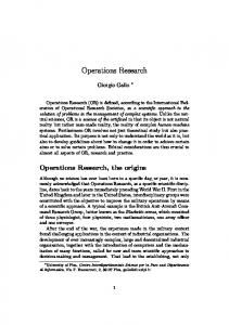
The lifecycle of an algorithm. . . . . . . . . . . . . . . . . . . . . . . . . . . 11

3.1

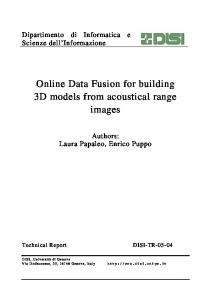
The architecture of Pentium III microprocessor. . . . . . . . . . . . . . . . . 33

4.1

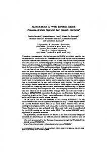
The main ideas behind the design of Catai. . . . . . . . . . . . . . . . . . . 48

4.2

A snapshot of Catai at start-up. . . . . . . . . . . . . . . . . . . . . . . . . 67

4.3

The scheme of the animation messages delivery. . . . . . . . . . . . . . . . . 68

4.4

The structure of an animated data structure.

4.5

The implementation of the paint anim links method in the graphWindow

. . . . . . . . . . . . . . . . . 68

class. . . . . . . . . . . . . . . . . . . . . . . . . . . . . . . . . . . . . . . . . 69 4.6

The definition of anim graph and some of its methods. . . . . . . . . . . . . 70

4.7

Prim’s algorithm for MST in its original (LEDA-like) version and its animation in Catai. . . . . . . . . . . . . . . . . . . . . . . . . . . . . . . . . . 71

4.8

Prim’s algorithm complex animation.

. . . . . . . . . . . . . . . . . . . . . 73

4.9

The animation starts on a graph. The priority queue is initialized by inserting in it each node of the graph with an initial cost set to the maximum allowed cost. All vertices in the graph are originally colored yellow, and all edges are colored black. . . . . . . . . . . . . . . . . . . . . . . . . . . . . . 74

4.10 Prim’s algorithm is running. The spanning tree grown so far has three nodes. Node 0 gives the current minimum light edge cost and is extracted from the priority queue. Light edges are colored CYAN in the graph window. 75 4.11 Node 0 is connected to the spanning tree using its light edge (0,5). All edges and nodes belonging to the solution are colored BLUE. . . . . . . . . 76 xii

4.12 We start exploring all the edges outgoing from the node 0 searching for its light edge. The currently selected edge, the one colored GREEN, is the new light edge for 0. It is colored CYAN. . . . . . . . . . . . . . . . . . . . . . . 77 4.13 Edges incident to node 4 are explored. Edge (6, 4) is the new light edge for node 6 and replaces the edge (6, 3) which is colored RED. . . . . . . . . . . 78 4.14 The algorithm has successfully computed the MST for the input graph. BLUE edges belong to the solution. 5.1

. . . . . . . . . . . . . . . . . . . . . . 79

ET and ST on random graphs with 2,000 vertices and different densities. Update sequences were random and contained 10,000 edge insertions and 10,000 edge deletions. . . . . . . . . . . . . . . . . . . . . . . . . . . . . . . 91

5.2

Experiments on random graphs with 2,000 vertices and different densities. Update sequences contained 10,000 insertions and 10,000 deletions. . . . . . 94

5.3

Experiments on random graphs with 2,000 vertices and different densities. Update sequences contained 10,000 insertions and 10,000 deletions: 45% of the operations were tree edge deletions. . . . . . . . . . . . . . . . . . . . . 95

5.4

Experiments on semirandom graphs with 2,000 vertices and 1, 000 edges. The number of operations ranges from 2,000 to 80,000. . . . . . . . . . . . . 96

5.5

Experiments on k-cliques graphs with inter-clique operations only. . . . . . 97

5.6

Experiments on k-cliques graphs with a different mix of inter- and intraclique operations. . . . . . . . . . . . . . . . . . . . . . . . . . . . . . . . . . 98

5.7

Experiments on worst-case inputs on graphs with different number of vertices. 99

6.1

Experiments on random graphs with 2,000 vertices and different densities. Update sequences contained 10,000 insertions and 10,000 deletions. . . . . . 106

6.2

Experiments on random graphs with 2,000 vertices and different densities. Update sequences contained 10,000 insertions and 10,000 deletions: 45% of the operations were tree edge deletions. . . . . . . . . . . . . . . . . . . . . 107

6.3

Experiments on semirandom graphs with 2,000 vertices and 1, 000 edges. The number of operations ranges from 2,000 to 80,000. . . . . . . . . . . . . 108 xiii

6.4

Experiments on several combinations of k-cliques graphs and a fixed number of of inter- and intra-clique operations. . . . . . . . . . . . . . . . . . . . . . 109

6.5

Percentage of time spent for keeping the list of non tree edges (dic) and for updating the MST solution (find) in the RR,RW,KQ cases. . . . . . . . . . 112

6.6

The implementation of the find root method. . . . . . . . . . . . . . . . . 117

6.7

The implementation of the common root ancestor method. . . . . . . . . . 121

A.1 The declaration of the EulerTour class. . . . . . . . . . . . . . . . . . . . . 129 A.2 The definition of the EulerTour class. . . . . . . . . . . . . . . . . . . . . . 134 A.3 The declaration of the ET tree class. . . . . . . . . . . . . . . . . . . . . . . 137 A.4 The definition of the ET tree class. . . . . . . . . . . . . . . . . . . . . . . . 142 A.5 The definition of the ETnode struct class. . . . . . . . . . . . . . . . . . . . 143 A.6 The declaration of the rnb tree class.

. . . . . . . . . . . . . . . . . . . . 144

A.7 The definition of the rnb node class. . . . . . . . . . . . . . . . . . . . . . . 149 A.8 The definition of the rnb node struct class. . . . . . . . . . . . . . . . . . 150 A.9 The definition of the st node class. . . . . . . . . . . . . . . . . . . . . . . . 151 A.10 The declaration of the ST tree class. . . . . . . . . . . . . . . . . . . . . 152

xiv

Chapter 1

Introduction

In the last decades we have witnessed an impressive interest into designing and characterizing efficient algorithms. Many interesting and significant achievements have been reached in several research areas as, for example, computational geometry, N P − hard approximation problems and cryptography. However, such wealth of results has not always been put in to practice or, in many cases, the experimental results did not meet the theoretical expectations. As a consequence, there is an increasing distance among theory and practice. The Algorithm Engineering is an emerging and promising discipline that proposes itself to narrow this gap by integrating algorithm experimental analysis into algorithm design. This should be accomplished by developing methodologies and tools that can be used both to put in practice theoretical results and to improve the comprehension of algorithms using experimental analysis. The Algorithm Engineering has been experiencing a general acceptance throughout the whole research community. One of the main problems it faces is the characterization of efficient algorithms. Several experiments conducted in the past have proven that, in some cases, the experimental behavior of an algorithm can be very different from the one predicted by the theoretical analysis, even in case of well coded implementations. Such consideration can be summarized as follows:

Optimal algorithms may exhibit experimental performances worst than the ones of other algorithms expected to be less performing with respect to the complexity analysis.

The main motivation for such a situation relies on the existence of the hidden constants.

Chapter 1. Introduction

2

These may dominate the experimental performances of an algorithm thus perturbating its behavior. However, it is a common expectation that the algorithm asymptotic behavior would still obey its complexity curve. At this point some considerations arise. First, what can we do if we are interested in using our algorithm in the range where hidden constants dominate? Second, what does it happens if this range is wide enough to cover any realworld application need? Third, even if the problem size grows it is not guaranteed that the algorithm performances will meet the predicted asymptotic behavior. This holds because increasing the problem size could unleash some other phenomena (e.g. computational overhead due to the virtual memory) that would degrade the algorithm’s performances. Indeed there is a dramatic need of a methodology for characterizing a realistic notion of efficiency.

1.1

Our Thesis

In our opinion, one of the main reasons for the situation described above is the increasing distance existing between the computational model used by the theoretical analysis and the real calculators’ architecture. The architecture of modern calculators has become much more complex than in the past, this happened both for the hardware and for the software layers. To face this problem, we promote the adoption of an investigation methodology able to fully characterize the experimental behavior of an algorithm. With the term characterization we mean the ability to fully annotate and understand the way an algorithm interacts with the underlying computational resources during its execution. Our approach relies on a redefinition of the commonly accepted notion of efficiency. Typically, it is considered efficient an algorithm requiring a low execution time. We believe that this notion should be integrated and improved by considering and analyzing the way the algorithm takes advantage from the available computational resources. Indeed, such an approach should require a better comprehension of the architecture of the real calculators. Even if not obvious, these considerations have been validated by our experience. As an example, we have found that even a vanilla-implementation of a simple minded algorithm performing very well in practice may hide a very bad usage of the available computational resources. The investigation methodology we define provides a qualitative approach to measure the performances of an algorithm so providing an in-depth fine-grained characterization. This


3

result has been made possible by the use of innovative analysis techniques and tools like hardware instruction counting and algorithm animation. While these techniques have already been available in the past years, they have been rarely used in this context. We believe they can give a non-trivial contribute to the problem of designing efficient algorithms. The application of our methodology not only allows to determine the efficiency of an algorithm but it also allows to achieve significant and non-trivial performance improvements. As a matter of fact, the application of our investigation methodology would serve for several reasons: • Algorithm performance evaluation Which criteria should be used to measure the performances of an algorithm? While it is easy to agree upon some generic statement like the amount of time the algorithm spent for its execution or the total amount of required memory, it becomes more difficult to define what we exactly mean with these statements. Instead, a qualitative approach allows to analytically describe which are the resources spent by an algorithm during its execution. As a results we are able to better recognize a ”good” algorithm. • Algorithm performance prediction As we previously said, complexity analysis may sometimes fail into predicting the experimental behavior of an algorithm. This mainly happens because of the computational model used during the theoretical analysis. This model is not able to take into account several factors that come into play during the execution of an algorithm. So, it becomes critical to understand which are these factors and in which way they influence algorithms. This knowledge help us to describe and to motivate the reasons why complexity analysis sometimes fails and how its predictions could be integrated in order to lead to a better comprehension of the algorithms’ behavior. • Efficient algorithms characterization Achieving a better comprehension of all the mechanisms that characterize the real performances of an algorithm is a challenging task. However, the ability to better predict and evaluate the performances of an algorithm is just one of the possible benefits. Let us suppose we exactly know which are the factors influencing the


4

performances of an algorithm, which way they work and which is their relative weight. Then, we can redefine the starting algorithm and its implementation taking enormous advantage from this knowledge.

1.2

The Organization of this Thesis

In the second chapter we will try to provide both a theoretical and practical modelization of a calculator. First, we will introduce the notion of computational model. We will discuss in detail the Random Access Machine model and the theoretical approach to the performance analysis of an algorithm. Then, we will try to characterize the architecture of a typical real calculator as it can be found nowadays. This work will help us to introduce all the technological features whose existence may have a significant influence on the behavior and on the performances of a running algorithm. The theoretical computational model and the real calculators’ architecture are then compared in order to emphasize the most significant differences and the way they could affect the traditional performance analysis. The chapter ends with a brief review of some of the alternative computational models proposed so far in order to solve the limitations of the RAM model. In the third chapter we will make some considerations about the notion of ”efficiency”. We will review the main existing techniques that can be used to monitor the performance of a running algorithm. Then, we will introduce the investigation methodology we have designed for achieving an in-depth characterization of the behavior of an algorithm. As we will see, the solution we propose acts at different levels of details providing both an overall characterization of the experimental performance of an algorithm and a fine-grained view so describing the way an algorithm interacts with the underlying hardware architecture. In the fourth chapter we will cover in details Catai, a tool we have developed for the animation of algorithms. It can be effectively used during the design of algorithms to provide an abstract representation of the behavior of an implemented algorithm. By so doing, it reveals to be a powerful tool to be used during the design and the engineering of an algorithm in order to verify its experimental behavior through an abstract intuitive graphical representation. In the fifth chapter we will present an extensive experimental study on dynamic graph algorithms. The presented work provides an experimental characterization of several algorithms for the problem of maintaining a minimum spanning tree on dynamic graphs. This work will


5

serve us both as an example of a typical experimental analysis and as a complex test bed for the experiments we will present in the following chapters. We have chosen the dynamic minimum spanning tree algorithms because they have some very nice features useful for our study. In the sixth chapter we will present the results of the experiments we have conducted. We have applied our investigation methodology to one of the algorithms seen in chapter two. We started the investigation by performing a traditional performance analysis on the target algorithm. Then, we isolated three significant case studies. These cases have been deeply analyzed so obtaining a fine-grained characterization of the algorithm behavior. Such work served us to reach a better comprehension of the algorithm’s performances. As a result, we have been able to understand which were the most critical operations together with their resource usage. Moreover, this analysis helped us to develop several optimizations able to significantly boost the performance of our algorithm. Finally, in the seventh chapter we will provide some conclusions about our work together with several interesting future research hints.

Chapter 2

Computational models: theory and practice

2.1

Introduction

Understanding the differences existing between abstract calculators and real ones is not an easy task. The theoreticians promoted the adoptions of abstract general computational models as the Random Access Machine. On the other side, real calculators’ architecture experienced a dramatic technological evolution. As a result, the gap existing between theory and practice has further widened. In this chapter we will try to outline these differences by introducing both the points of view and by discussing their main characteristics. To this aim, we will investigate the RAM computational model and the principles of worst case analysis, one of the most used algorithm analysis technique. Then, we will introduce the typical architecture of a real calculator. We will focus on those aspects that, in our experience, may have a significant impact on the performances of an algorithm. This discussion will allow us to compare both the RAM computational model and the typical real machine hardware and software architecture. The results of this discussion will serve us in the next chapters as a basis for our experiments. As a conclusion, we will provide some details on alternative computational model as the Parallel Disk Machine that can be used, in some cases, to better describe the architecture of a real calculator.

2.2

The Random-Access Machine Computational Model

A computational model can be defined as a formal language to be used for writing programs. Such programs can be run using an abstract idealized machine with unlimited time and memory resources. The Random Access Machine (RAM) model [4] defines a

Chapter 2. Computational models: theory and practice

7

basic calculator able to operate on an unbounded sequence of registers holding integer values. Each integer register can be accessed at the same time. Moreover, the calculator features also an instruction counter, one or more accumulator registers and a program to be executed. The instruction set of a RAM features arithmetical operations for accessing and modifying the contents of the registers. These operations work by transferring the content of a memory cell to one of the available accumulators. Instructions are executed in sequential order and they require all the same execution time. Conditional and iterations statements are available too. A RAM calculator has the same computational power of a Turing machines since this one can be emulated using its instruction set.

2.2.1

Evaluating the running time of an algorithm

The running time of an algorithm run on the top of a RAM could be trivially characterized by evaluating the sum of all the operations required for its execution weighted with their execution time. To this end, we should know the size of the input problem to be solved. However, if we are interested into providing a more general characterization of the efficiency of the algorithm then we should evaluate its performances for all the possible inputs. Obviously, this is not a realistic approach; in these cases it is convenient to use a more general characterization. To this end, Knuth introduced the theory of the analysis of algorithms [9, 10, 11]. Knuth himself provided the following remarks while speaking of analysis of algorithms [8].

People who analyze algorithms have double happiness. First of all they experience the sheer beauty of elegant mathematical patterns that surround elegant computational procedures. Then they receive a practical payoff when their theories make it possible to get other jobs done more quickly and more economically

Analysis of algorithms is usually accomplished by using complexity analysis. This technique evaluates the performances of an algorithm by bounding its running time (time complexity) or the memory required for its execution (memory complexity) to the size of input problem. Under these assumptions, the complexity analysis determines a function defining the relation between the size of the input problem and the amount of resources required for its solution.


8

However, since an algorithm may exhibit a very different behavior according to the input data set we have in some way to distinguish among ”good” inputs and ”bad” inputs. This is usually done by analyzing an algorithm according to different typologies of data sets. We can distinguish the following kind of analysis:

• Worst-case analysis It studies the behavior of an algorithm when facing a problem that maximizes the number of steps required for its execution. • Best-case analysis It studies the behavior of an algorithm when facing a problem that minimizes the number of steps required for its execution. • Average-case analysis It studies the behavior of an algorithm in the average case (i.e. we suppose the input data set to be chosen according to some probability distribution).

The kind of analysis typically used is worst-case one because it provides an upper bound of the running time of an algorithm. Speaking of the running time analysis, Rivest et al. [6] observed that, for large enough inputs, the multiplicative constants and lower-order terms are dominated by the effects of the input size itself. If we are interested into studying and characterizing the behavior of an algorithm when the size of the input problem increases without bounds then we can ignore lower-order terms and multiplicative constants because they become insignificant. Obviously, these factors have still a meaning in the original algorithm and their influence can have a significant impact on the performances of an algorithm, especially for small input data sets. The notions introduced above lead us to the concept of asymptotic efficiency of an algorithm. The asymptotic behavior of an algorithm can be described with the help of the big-Oh notation (see [6]). In few words, the big-Oh notation allows us to describe the complexity function of an algorithm by replacing it with the one of another algorithm whose behavior is asymptotically very similar but that is much more simpler to characterize.


2.3

9

Some of the Limitations of Complexity Analysis

As we already said, the complexity analysis determines the efficiency of an algorithm by bounding its asymptotic running time of an algorithm. While this approach works well in theory, it may not fit well in the practice. As pointed out by Tamassia et al. [20], it is quite common for algorithms that have been declared “asymptotically optimal” in the Random-Access Machine (RAM) computational model to be inferior to “suboptimal” algorithms in practice. There are several reasons for this to happen. First of all, it must be said that it is not always possible to find a tight enough bound for the running time of an algorithm. Let us consider, as an example, the case of the simplex method. This algorithm features an exponential time worst case however it performs much more better in practice exhibiting a polynomial time behavior [13, 19]. Speaking of the asymptotic analysis, sometimes an algorithm may exhibit its asymptotic behavior only when facing very large input problem. Moret [16] cites the case of the Fredman and Tarjan algorithm [15] for minimum spanning trees. Its asymptotic running time is O(|E|β(|E|, |V |)) where β(n, n) is given by min{i| log(i) } with n ≤ m/n, so that β(m, n) is log∗ n. For dense graph, this bound is much better than the ones of Prim’s algorithm. However, experimental analysis has proven that the crossover point between the two algorithms occurs only with dense graphs having billion of edges. A similar example can be introduced regarding hidden constants, Robertson and Seymour give a cubic time algorithm [18] for proving if a graph is a minor of another. The size of the hidden constants has been estimated in 10150 , large enough for dominating the performances of the algorithm on every real life problem.

2.4

The Architecture of a Modern Calculator

Providing a general and complete characterization of the experimental computational framework for an algorithm is not an easy task. This happens for several reasons. First, the hardware architecture of computers has radically evolved in the last decades with respect to the first sequential calculators. Current calculators implements so much hardware optimizations and tricks they could barely resemble the original calculators. Second, while the theoretical computational model provides a clean, abstract and general formalization of a calculator, in the real world the situation is much more complex. Even with


10

the general acceptance of several architectural patterns, there does not exist a general standard-computer architecture. As a result, every investigation in this field requires an ad-hoc analysis. Finally, these considerations must also cover the operating system and application software layer. This holds because, nowadays, algorithms are coded using high level programming languages and executed in multi-tasking environments. These factors may have a considerable effect on the performances of the algorithms. For all the reasons cited above it is quite difficult to provide a concise and exhaustive generalization of the experimental framework used during the execution of an algorithm as we have already done in the theoretical case with the RAM computational model. In the following sub sections we try to provide a sort of generalization of the hardware/software architecture of the modern calculators. This work has been done considering both the technological patterns that are commonly applied and the lifecycle of an algorithm as illustrated in Figure 2.4. We have put a strong emphasis on those aspects that, in our experience, may have a significant impact on the characterization and on the performances of an algorithm. In chapter 3 we will provide a more detailed explanation of the experimental framework we have used during our work.

2.4.1

Hardware platform

The hardware platform provides the effective computational resources to be used during the execution of an algorithm. It is probably the element whose characterization is most difficult. The modern calculators implement a consistent amount of technologies aimed to maximize the program’s performances and improve the effective usage of available computational resources. All these technologies contribute with a consistent boost of the efficiency of the overall system but, at the same time, they increase the distance with respect to the theoretical RAM model. We report some of the most significant technological features: • Instruction scheduling This technique allows the processor to redefine the order the input assembler instructions will be executed. This is especially useful when the execution of an instruction cannot take place due to a memory stall (i.e. the needed data must be fetched from the memory).


11

Figure 2.1: The lifecycle of an algorithm. • Superscalar execution A superscalar processor is able to issue multiple instructions in a parallel execution. Parallelism is achieved by replicating the operational components of the processors. This technology relies on the the ability of the instruction scheduling techniques to provide a batch of assembler instructions that can be executed in any order, even at the same time. For instance, the most recent processors are able to execute up to six instructions at the same time. • Very Long Instruction Word architectures Some of the most recent microprocessors are able to pack into a single macroinstruction several operations to be performed in parallel. For this reason, they use very long instruction word (VLIW). This feature can be seen as an evolution of traditional superscalar microprocessors. The main differences resides in the parallelization of the source code. In the VLIW architectures the high-level programming language compiler or pre-processor breaks program instructions into multiple basic


12

operations that are coded into a single very long instruction and then executed in parallel. • Speculative execution This technique allows the processor to predict the resulting value of a function not yet evaluated. Such a feature reveals to be crucial while facing conditional branches. In this case, the processor is able to predict the result of the branch and, then, to proceed with the execution of the code. The prediction scheme usually takes advantages of an history buffer used to remember the branches already taken in the past. If the prediction fails, the processor has issues a roll-back discarding the last instructions executed. • Single Instruction Multiple Data Instructions The Single Instruction Multiple Data (SIMD) instructions are able to apply a same operator on several data at once. This means that is possible to perform the same operation in one shot on a batch of data. This is extremely useful for multimedia applications where, typically, there is need to independently apply the same operator to a large amount of data.

2.4.2

Memory hierarchies

The memory subsystem is one of the most crucial components in modern calculators. The availability of different memorization technologies has led to the definition of a vertical hierarchical model for storing both data and instructions. Each level of this hierarchy features different methods and timings for accessing and updating the contained information. Generally, higher levels feature faster and more expensive memory than lower levels. As a result, accessing a single element into memory could require from a clock cycle to several thousands cycles according to the memory position of the element to be retrieved. Memory management, both at the hardware and software level, is accomplished so to maximize the probability that the needed information, either data or instructions, could be found on the highest level (i.e. the most performing one). In order to achieve this result, memory hierarchies take advantages from the concept of locality. According to this concept, a memory element that has been accessed recently will be likely accessed


13

soon (temporal locality) and, given a memory access, the elements stored near the accessed element have a good probability of being used soon (spatial locality).

2.4.3

Operating system

Modern operating systems implement a framework where multiple processes can share the same computing and memorization resources in a transparent and safe way. For this reason, they are designed using a layered architecture. Lower layers are interfaced with the computational resources and are in charge of defining the kernel of the operating system. Upper layers present an abstract hardware-independent interface to be used by processes for accessing computational resources. Each process is executed in a virtual environment that allows to access memory, storage devices and CPU without caring of the other processes. We briefly introduce the two principal technologies used to implement such features: • Virtual memory Virtual memory allows a process to allocate and manipulate an amount of memory limited only by the machine word length and by the amount of available secondary memory. The traditional implementation of virtual memory organizes the main memory into pages of equal size, each of them labeled with a unique id. Memory requests coming from processes are satisfied by allocating a proper number of pages. If there is not enough main memory to satisfy a new request then some of the existing pages are swapped on the secondary memory so to free the needed pages. The pages to be swapped are usually chosen among the ones with the least probability to be used in the next future. It is possible to implement virtual memory in a transparent way for the processes by using logical addressing. A logical address is made of a pair reporting the page id and the offset inside the page. This technique requires the operating system to maintain a table mapping each page id into a real memory base address. For this reason, each memory access made into a system using the virtual memory requires an additional overhead needed for the table lookup. This overhead could further increase if the required page is not present in the main memory. In this case it must be considered the time needed to swap the page to be loaded from


14

the secondary memory with the one selected for the substitution.

• CPU scheduling and Context Switches The implementation of a multi-tasking operating systems requires that the computational resources offered by a calculator should be transparently made available to all existing processes. The main resources to be shared are the CPU and I/O devices. The technologies developed so far aim to optimize the usage of the computational resources and to maximize the number of atomic computational unit (job) served in a fixed interval of time. The sharing of the CPU is achieved by adopting a proper scheduling algorithm. In order to be multi-tasking, an operating system has to support context switches. These operations freeze the execution of a running process scheduling the CPU access to another process. Before passing the control to the new process, a context switch has to save all the information describing the state of the current process. This operation is not trivial and can imply a significant overhead. Let us consider, for example, processes with many I/O operations; these processes suffer frequent context switches thus paying a consistent computational overhead.

2.4.4

Developing platform

The coding of an algorithm is usually perceived as a sort of automatic step consisting of a direct translation of the algorithm into an equivalent implementation. However, this phase should not be underestimated since both the choice of the programming language and the subsequent implementation of the algorithm may hide many pitfalls. In fact, the choice of the programming language has an intrinsic impact on the performances of the algorithm to be implemented. As an example, the current technological trends seem to prefer the adoption of very high level and abstract languages able to reduce the coding time, minimize the cost of multi-platform developing and to improve the productivity of the developers. Such sophistications have a cost since this solution restricts the possibility to directly interact with the underlying hardware widening the gap existing among the source code high-level definition of an algorithm and the final code to be executed. In the same way, many high-level significant features like Object Oriented programming paradigm, virtual machines and dynamically loadable code may penalize the performances of an algorithm.


2.4.5

15

Support libraries

The most part of the existing algorithms share a common subset of elementary data structures, we cite as examples: linked lists, hash tables and binary trees. To avoid recoding them at any algorithm implementation, these data structures are usually coded as standard reusable components and, then, packed as libraries of data structures. The role of these components is crucial since almost every algorithm, even the most complex, spends the greatest part of its execution using elementary data structures. In order to enhance both reusability and portability these library are typically coded using high-level Object Oriented programming languages. This implies that components designed keeping in mind portability and reusability may exhibit very poor performances. This approach has even some other dangerous side effects: pre-coded data structures are used as black box components while their implementation is often unknown. This means that we are not able to know exactly the behavior of these components neither we are able to motivate their performances.

2.5

The RAM Computational Model vs. the Real Calculators’ Architecture

At this point we are ready to make some first considerations about the most significant differences existing among the RAM computational model and the typical architecture of a modern calculator. • Atomic instructions In the theoretical approach an algorithm definition can be provided by using RAM instructions all having the same execution time. Real calculators split the execution of each assembler instruction into several stages, the number of cycles needed to execute an instruction may change according to the complexity of the operation. Moreover, algorithms are implemented using high-level programming languages. This implies that an algorithm atomic step could be translated into several, even complex, assembler instructions.


16

• Sequential execution As we have seen, the RAM model features a strictly sequential execution. On the other hand, a superscalar architecture provides a processors with several execution pipes in order to execute multiple instructions at once thus implementing a true parallel execution.

• Instruction order execution In the RAM model instructions are issued and executed in the same order they were provided as input code (In-Order execution). On the contrary, real calculators allow instructions to be executed in a different order (Out-of-Order execution) than the one provided as input.

• Memory references The RAM model adopts a flat modelization of the memory. All memory references have the same cost. On the contrary, real calculators have their memory organized using an hierarchical structure. Access time to memory locations belonging to different levels of the hierarchy may vary with several different orders of magnitude.

There are several cases of algorithms that have been able to take advantage from these differences in order to exhibit optimal performances not predictable using the traditional RAM model. We cite, as an example, the work of Andersson et al., they proposed a very efficient sorting algorithm[3] using packed computation. They take advantages of the word length of current microprocessor to stuff into a single word multiple data at once. Then, they provided a simple algorithm to perform multiple comparison in parallel while performing a single mathematical operation. Another interesting example has been provided by LaMarca et al. with their study on the influence of the caches on the performance of sorting[14]. They proved that non-comparison based algorithms like the radix-sort exhibit very poor performances with respect to their comparison-based counterparts due to their intrinsic bad usage of the cache memories.


2.6

17

Alternative Computational Models

The RAM based computational model has been widely accepted in the scientific community however, as we already said, it is not able to describe even some of the most common technological features of currently available calculators. This problem could be solved by adopting an alternative and more realistic computational model. To this end, several computational models have been proposed in the past decades. The most part of them provides a modelization of parallel machines and their communication complexity. We cite as an example, the Bulk Synchronous Parallel model proposed by Valiant [21] and the LogP model proposed by Culler et al [5]. Speaking of the sequential case, we cite the Hierarchical Memory Model (HMM) defined by Aggarwal et al [2]. They introduced a model where all operations are executed sequentially by means of a single CPU, memory accesses have a variable cost according to the location of the referenced element. In the HMM model the access time to a memory location x can be determined evaluating an access cost function f (x). Typical access cost function are log(x) and xα with α > 0. An evolution of the HMM model has been presented by Aggarwal et al [1], it takes into account block transfer memory accesses and it is so referred as BT. This model starts from a consideration, the access to an element in a real memory system causes the whole block of data containing the element to be fetched. As a result, accesses to contiguous memory locations are much less expensive than accesses to random locations. Let be t a set of memory locations to be accessed and x the location of the last element then accessing the t elements would require f (x) + t time in the BT model where f (x) is the same access cost function seen in the HMM model. Another significant contribution is the Parallel Disk Model(PDM) introduced by Vitter et al [22, 23]. This model can be used to evaluate the performances of algorithms working on external memory or just using disk devices as memory extensions in virtual memory environment. It starts from the premises that the size of the input problem is greater than the size of the RAM memory available. As a consequence, they provide a model where an algorithm can explicitly control data placement and retrieval over several storage devices. They introduce a set of primitive operations like read or write that can be used for transferring to or from the storage devices blocks of data. One of the main ideas is to take advantage from the existence of several independent storage devices in order to perform parallel efficient disk accesses. To this end, informa-


18

tion is not written all together on a single disk, instead it is striped over the whole set of available devices. This model uses as performance metrics three machine-independent measures, namely these are: number of I/O operations, CPU time and amount of used disk space.

References

[1] A. Aggarwal, B. Alpern and M. Snir, “Hierarchical Memory with Block Transfer”. In Proc. of 28th Annual IEEE Symposium on Foundations of Computer Science, pages 204-216, October 1987. [2] A. Aggarwal, B. Alpern, A.K. Chandra and M. Snir, “A model for Hierarchical Memory”. IBM Watson Research Center, Technical Report RC 15118, October 1989. [3] A. Andersson, T. Hagerup, S. Nilsson and R. Raman, “Sorting in Linear Time?”, ACM Symposium on Theory of Computing (STOC), 1995. [4] S.A. Cook and R.A. Reckhow,“Time bounded random access machines”.Journal of Computer and System Sciences, 7(4):pages 354-375, August 1973. [5] D. Culler, R. Karp, D. Patterson, A. Sahay, K. E. Schauser, E. Santos, E. Subramonian and T. von Eicken, “LogP: Towards a Realistic Model of Parallel Computation”.In Proc. of the Fourth ACM SIGPLAN Symposium on Principles and Practice of Parallel Programming, pages 1-12, May 1993. [6] T. H. Cormen, C. E. Leiserson and R. L. Rivest, “Introduction to Algorithms”. Mc Graw-Hill, 1990. [7] J. L. Hennessy and D. A. Patterson, “Computer Architecture: A Quantitative Approach” 2nd edition. Morgan Kaufmann, 1996. [8] D. E. Knuth, “Selected Papers on Analysis of Algorithms ”. Stanford, California: Center for the Study of Language and Information, xvi (CSLI Lecture Notes, no. 102.), 2000.

References

20

[9] D. E. Knuth, “The Art of Computer Programming: Fundamental Algorithms”. Addison-Wesley, 1973. [10] D. E. Knuth, “The Art of Computer Programming: Seminumerical Algorithms”. Addison-Wesley, 1981. [11] D. E. Knuth, “The analysis of algorithms”. In Actes du Congr’es International des Math’ematiciens, Nice, France, pages 269-274, 1970. [12] D. E. Knuth. “The Art of Computer Programming: Sorting and Searching”. AddisonWesley, 1973. [13] V. Klee and G. J. Minty, “How good is the simplex method?”. In Shisha, O. editor, Inequalities - III, Academic Press, pages 159-175, 1972. [14] A. LaMarca and R. Ladner, “The influence of caches on the performance of sorting,” In Proc. of8th ACM/SIAM Symp. on Discrete Algs. (SODA 97), pages 370-379, 1997. [15] B. M. E. Moret and H.D. Shapiro, “An Empirical Assesment of algorithms for constructing a minimal spanning tree”. In Computational Support for Discrete Mathematics, N. Dean and G. Shannon, eds.,DIMACS Series in Discrete Mathematics and Theoretical Computer Science 15, pages 99-117, 1994. [16] B. M. E. Moret, “Towards a Discipline of Experimental Algorithms. In DIMACS Monographs in Discrete Mathematics and Theoretical Computer Science, 5th DIMACS Challenge. American Mathematical Society, 2000. [17] K. Wagner and G. Wechsung, “Computational Complexity”. D. Reidel, Dordrecht, 1986. [18] N. Robertson and P. Seymour, “Graph minors: a survey”. InSurvey in Combinatorics, Cambridge Press, pages 153-171, 1985. [19] D. A. Spielman and S. Teng, “Smoothed Analysis of Algorithms: Why the Simplex Algorithm Usually Takes Polynomial Time”. [20] R. Tamassia, P. K. Agarwal, N. Amato, D. Z. Chen, D. Dobkin, R. L. S. Drysdale, S. Fortune, M. T. Goodrich, J. Hershberger, J. O’Rourke, F. P.

References

21

Preparata, J. R. Sack, S. Suri, I. G. Tollis, J. S. Vitter, and S.Whitesides, “Strategic Directions in Computational Geometry Working Group Report”. http://www.cs.brown.edu/people/rt/sdcr/report/report.html, 1996. [21] L. G. Valiant, “A Bridging Model for Parallel Computation”. In Communications of the ACM, 33:8, pages 103-111, August 1990. [22] J. S. Vitter and E. A. M. Shriver, “Algorithms for Parallel Memory I: Two-level Memories”. Algorithmica 12:2/3, pages 110-147, August and September 1994. [23] J. S. Vitter and E. A. M. Shriver, “Algorithms for Parallel Memory II: Hierarchical Multilevel Memories”.Algorithmica, 12:2/3, pages 148-169, August and September 1994.

Chapter 3

Characterizing an efficient algorithm

3.1

Introduction

As we have seen in the previous chapters, the theoretical way to algorithm performance analysis makes use of the asymptotic running time analysis: it determines the best algorithm by choosing the one whose running-time order of growth is better. In the real world, characterizing an efficient algorithm is not an easy task. Due to the complexity of the underlying hardware and software architecture, an optimal algorithm could perform very bad on a real calculator. At the same time, a simple-minded algorithm may be able to perform better thanks to an improved usage of the available computational resources. This is the case of the algorithm for maintaining the MST of an input graph using the Euler Tour trees seen in the chapter 5. As a consequence, the evaluation of an efficient algorithm from an experimental point of view cannot be just performed by evaluating running time but it must take into account even how efficiently the algorithm interacts with the available computational resources. This requires a strong characterization of its experimental behavior. By this term we mean the ability to identify the resources consumed during the execution of an algorithm and analytically describe the way they are used. In this chapter we will introduce some of the traditional approaches to the experimental performance evaluation of algorithms. We will present several metrics useful to rate the performances of an algorithm. We will then discuss the available techniques for measuring the experimental performances of an algorithm. This discussion will lead us to the introduction of the investigation methodology we have defined. Our approach allows one to perform a fine-grained effective analysis of the performances of an algorithm. Instead of using a single metric, our approach characterizes the behavior of an algorithm by

Chapter 3. Characterizing an efficient algorithm

23

integrating several different kind of analysis. One of the main advantages of our solution is the detail level achievable while investigating the resources usage of a running algorithm. This has been made possible by the use of the performance counters, these are special purpose register commonly found in the most recent processors and able to describe the interactions of a process with the underlying hardware. Finally, we will present the experimental framework we have set up to apply our investigation methodology. We will cover all those aspects who will be critical in the experiments we will present in the chapter 6.

3.2

What to Measure?

There are many ways to rate the performances of an algorithm. A traditional approach is to measure the total amount of time and memory required for its execution. This is a widely accepted solution and it seems to answer well to questions like ”which is the best algorithm?”. Nevertheless, this approach may have several different interpretations. In a multi-tasking operating system measuring the total time needed by the algorithm to finish its execution could not be enough, several other processes may have delayed the algorithm execution time. A smarter approach would be to measure just the time a process spent executing the algorithm while in user mode. However even this approach has some disadvantages, an algorithm working with very large data structures may have a very little execution time but a much longer overall execution time due to disk accesses. A different approach would be to measure the performances of an algorithm as the exact amount of machine language instructions issued during the execution of a program. In this way we have a deterministic characterization of the workload needed for executing an algorithm. This approach is very interesting since it resembles the one used in the RAM model to characterize the exact running time of an algorithm but it is very difficult to be applied. This holds because of the architecture of the modern processors; superscalar execution and memory hierarchies are far too complex to be easily taken into account. There is a completely different and orthogonal approach based on the measurement of the low level resources spent during the execution of an algorithm. For example, we could measure the total number of processor cycles needed for the execution of an algorithm. In this case we have a more precise performance estimation. Such an estimation could be further integrated by measuring also other resources like the total number of instructions exe-


24

cuted and the cache usage profile. This approach has not been widely accepted for several reasons. First of all, there are some serious technological difficulties, low-level resource monitoring is often not supported or unavailable at operating system level. Moreover, the information collected with this technique are difficult to be interpreted, especially when applied to complex algorithms. These considerations convinced us to not rely on a single metric to rate the efficiency of an algorithm. On the contrary, the approach we propose integrates the traditional analysis techniques with the low-level resource monitoring. As a result, we provide a characterization technique based on the estimation of several indexes describing the interaction between the algorithm code and the underlying calculator weighted with the size of the problem to be solved.

3.3

Performance Evaluation Techniques

Several techniques for the acquisition of information describing the behavior of an algorithm have been proposed so far. We describe the most used and interesting ones.

3.3.1

Profiling

A profiler [14, 15] allows the gathering of statistics about the execution of a target program. Traditional profilers take as reference the source code formulation of the observed program. The resulting statistics report the number of times each functional block of the program has been called and the amount of time spent for their execution. There are two main profiling techniques. Sampling profiling periodically interrupts the execution of the target program. After each interruption, the call-trace stack of the program is examined in order to determine which function is being executed. It is possible to guess the execution profile of the program by repeating the sampling during the whole execution of the algorithm. The approximation degree of this technique is as low as the sampling interval of time is longer. This reveals to be a problem when we are interested in describing the behavior of very short functions, in this case the profiler may be unable to discover even the execution of such functions. This happens because short functions may be entirely executed among two distinct sampling thus being unobservable by the profiler. Trap profiling works by executing a special profiling function each time a functional block is entered or left. The profiling function is in charge of recording the identity of the current functional block in


25

order to rebuild the call-graph map. Moreover, each time the program enters a functional block, a time stamp is set in order to guess, after the program leaves the functional block, the amount of time spent for its execution. Trap profiling is far more precise than sampling profiling but requires much more overhead. This technique can be used only to perform an high-level analysis of the behavior of an algorithm. It is only possible to know the resource usage of blocks of code while nothing can be said about the resource usage of single instructions.

3.3.2

Program Tracing

Program tracing [5, 20] requires the program code to be enriched with special tracing instructions in charge of recording relevant events describing program activity. Each event reports a time stamp and its identity. It is possible to describe the program behavior by performing a post-mortem analysis of log data. This technique can be considered as a derivation of standard profiling techniques. The main difference resides on the kind of report activity and on the overhead required by the measurement. This is especially true if we consider that, differently from profiling, a the event generation may be a very light activity thus having a very low impact on the performances of the observed algorithm.

3.3.3

Simulation

This technique relies on the use of a software program (simulator) in order to simulate a computational, memory or communication resource used during the execution of a program. The target program is executed on the top of the simulator, all the interactions with the simulated resource are recorded. Simulation has two main purposes: to allow the monitoring of low-level hardware resources and to minimize the overhead needed to monitor the program activity. Moreover, when using simulation it is possible to experiment the behavior of a program on different hardware configuration by just triggering some of the simulation parameters (e.g. amount of available cache memory, latency for memory accesses). There are two possible approach to performance evaluation through simulation: • Partial Simulation It is typically used to model memory or communication resources like cache memories or network channels. The program targeted for the execution must be interfaced in


26

a transparent way to the simulator. This may happen by automatically instrument the program code with special-purpose simulator directives or by replacing standard system libraries with special ones supporting the simulator. • Total Simulation The simulator creates a virtual environment simulating a whole calculator. It is possible to install both the operating system and the needed support software on the top of a running instance of the simulator. This framework allows the execution of whatever software designed to work with the simulated calculator. However, since the whole hardware layer is simulated, it becomes possible to know exactly which are the resources spent for the execution of a program.

Both the approaches presented above are difficult to implement. The increasing complexity of real calculators makes it very problematic to build a full-featured simulator. For these reasons this technique is mainly used to simulate and to study only some critical components of a calculator such as the cache memory hierarchy.

3.3.4

Hardware Instruction Count

This technique relies on the use of the Hardware Performance Counters (HPC) [6, 10, 26]. These are hardware registers available on almost all the recent microprocessors. They can be used to analytically describe the activity of a microprocessors by means of events measurements. Each HPC can be programmed to monitor a given event then, each time the event occurs the counter is increased. The granularity level of these counters is very high since they allow to monitor very low-level activities like the total number of cache accesses or the total number of assembler branches during the execution of a program. The main advantages of this technique are both the detail level achievable and the possibility to perform an hardware based observation that has a very low impact on the performances of the observed program. However, the granularity is also one of the main problem of this technique. While such a deep characterization is very useful to study little pieces of code, it could be too much overwhelming and misleading for complex algorithms.


3.4

27

Our Approach

The investigation techniques introduced so far can be useful to focus only on some details of an algorithm performances without being able to characterize the overall behavior. For this reason, we developed an experimentation framework that allows us to study the behavior of an algorithm with different levels of details and granularity. To this end, our framework supports five types of investigations:

3.4.1

Overall algorithm behavior

This is the traditional investigation consisting of a quantitative sampling of the performances of the algorithm as it can be accomplished from the operating system point of view. The algorithm performances are described measuring the total resources usage like the execution time and the memory usage. In order to have a better characterization of the execution time we measure the total execution time of the process running the algorithm, the time the process spent while in user mode and the time the process spent in system mode. The memory usage is sampled as the maximum amount of memory allocated to the process during its execution. What we do is to iterate the execution of an algorithm on a batch of input data sets of increasing size. These data allow a first description of the algorithm performances; to this end, they can be plotted and then compared with the theoretical analysis expectations.

3.4.2

Functional blocks investigation

At this level, we investigate the behavior of the algorithm as it is implemented in a highlevel programming language. Namely, we trace the amount of resources needed for the execution of the functional blocks composing the program implementing the algorithm by using standard profilers . The resulting information can be used to characterize the behavior of whole blocks of the input algorithm as the size of the input problem changes. This technique reveals to be extremely useful to find large performance bottlenecks together with providing a first coarse-grained insight of the algorithm experimental behavior.


3.4.3

28

Algorithm oriented investigation

In order to understand which has been the behavior of a running algorithm we cannot just rely on the execution time. There is a significant class of information whose collection cannot be automated thus requiring specific code instrumentation. We are speaking of all those information describing the experimental state of the algorithm data structures. These information are crucial if we want to be sure that the experimental behavior of the algorithm follows its abstract formulation. For example, we could be interested in knowing the mean height of a dynamic binary randomized tree used by a running algorithm. These information can be collected by properly enriching the original source code of the algorithm we want to investigate. In this way we are able to fully browse the internal state of the algorithm and of its data structures. The information so generated are collected, organized and represented using text-manipulation oriented scripting languages and statistical analysis tools.

3.4.4

Algorithm Animation

The algorithm animation is a technique to be used to produce graphical visualizations of input algorithms. Consider that the code implementing an algorithm is usually complex to be interpreted since it hardly resembles its abstract formulation. The same happens during the execution of an algorithm, even the most complex debugger can only provide an implementation and hardware oriented representation of the state of an algorithm. these situations, the algorithm animation reveals to be a very efficient tool since it can provide an abstract representation of the behavior of a running algorithm through a graphical visualization. In such a way it becomes possible both to easily check if an algorithm is performing as expected and to check if some invariants are maintained (e.g. color properties in a red-black tree).

3.4.5

Analytic investigation

While the previous investigation levels are able to provide an extensive characterization of the algorithm state and behavior, they are unable to offer an in-depth low-level characterization of the resources usage. This is especially true if we consider that standard high


29

level programming languages instructions are usually converted into several, even complex, assembler instructions. In the same way, as it happens for the overall execution time of an algorithm, there are some cases where we cannot just summarize the performance of a statement by using a single quantitative metric. Let us consider, as an example, the operation of accessing an element into an hash table. Apparently, this operation requires only a single step. However, computing the hash function and accessing the data elements may require additional, unpredicted, overhead. In these cases we have to operate a fine-grained investigation analyzing the way the observed instructions interact with the underlying hardware. To solve this problem, we introduce the use of Hardware Performance Counter(HPC) to collect information about critical portions of code. Namely, we gather the following information during the execution of an algorithm: • Total number of cycles This metric reports an exact count of the cycles the processor spent while executing the code of the algorithm. This is one of the main metric we used during our work. In fact, this estimation is much more precise than the operating system level time measurements. However, we could be tempted to obtain a real time estimation by multiplying the total number of cycles for the duration of each cycle. This solution is not correct since actual superscalar processors are able to execute multiple instructions at once as we have seen in 2.4.1. • Total number of Instructions Issued This metric reports the total number of assembler instructions issued during the execution of the algorithm. This information provides us only a quantitative characterization of the ”work to be done” for the execution of the algorithm. This happens because the instructions describing the algorithm have different execution times. However, we can combine this metric with other ones as the total number of cycles to obtain an estimation of the performances of the processor during the algorithm execution. • Total number of Level 1/2 Cache Accesses Memory references are usually the most frequent operations occurring during the execution of an algorithm. This happens because almost every assembler instruction


30

needs to fetch some arguments from the memory. As a result, this metric can be used instead of the total number of instructions issued to characterize the workload needed for the execution of a target algorithm. • Total number of Level 1/2 Cache Miss As long as being one of the most frequent operations, memory accesses are also among the most expensive instructions due to cache misses. While a miss on Level 1 cache costs only a limited number of CPU cycles, a miss on Level 2 cache may cost even hundreds of CPU cycles. An algorithm with a bad memory organization may exhibit very poor performances. For these reasons it becomes critical to be able to measure how many misses there have been during the execution of an algorithm. Such measurement is interesting not only as a single metric but also combined with the total number of instructions issued and with the total number of cache accesses in order to determine how well the algorithm is able to use the cache memories. • Total number of stall cycles This metric reports an exact count of the cycles the processor spent idle while waiting for a data from the memory system. Using this information we could rate the efficiency of the processor with respect to the program being executed. The total number of stall cycles can be combined with the total number of execution cycles in order to obtain an overall efficiency measure. • Cycles per instruction This metric describes the efficiency of the considered program when run on the top of our experimental framework as follows: total number of instructions total number of cycles The relevance of this metric is undoubtful. Remember that super scalar microprocessors are able to process in a clock cycle multiple instructions whose execution requires several cycles. The cpi metric is able to describe how efficiently a target program uses the underlying computational resources. As reported by Patterson in [19], a more accurate evaluation of the cpi for a code could require to distinguish among the cpi of the memory system and the cpi of the processor. However, in our


31

work, we have considered the most simple and general interpretation of cpi since it fits well enough our needs. As a result, we get a very detailed description of the hardware interactions occurred during the execution of the observed instructions. While it is tempting to use this technique to characterize the overall behavior of an algorithm, we point that such technique would be too much time-consuming and complex to be interpreted. Conversely, this technique reveals to be very useful on a small-scale.

3.5

The Experimental Framework

The definition of the experimental framework is a crucial task. As we have said before, there are many factors influencing the behavior of a running algorithm. We had to make a choice regarding the factors to study. We have chosen to restrict our investigations on the way the algorithm code interacted with low-level computation resources, including in this definition both the processor activity and the memory system usage. Our testing platform uses a Pentium III (P3) based Personal Computer equipped with 1 Gb of physical RAM and the Linux [21] operating system installed on. We have used the C++ programming language as it is implemented by the gcc compiler [13, 25] with the support of both the LEDA library [22, 23] and the dynamic graph Leda Extension Package [1] to develop test algorithms. The overall characterization of the algorithm’s performances has been conducted with the help of the standard UNIX system calls. The gprof [14, 15] tool has been used together with an ad hoc profiling library to accomplish the functional block investigation. Finally, the analytical investigation has been conducted with the help of the PAPI [2, 3, 4] library, a standard API to be used for accessing Hardware Performance Counter available on Intel processors. In the following sub sections we will discuss the peculiarities of our experimental framework, focusing our attention on the processor and the memory system.

3.5.1

The processor architecture

The processor Pentium III (P3) [11, 7, 8, 9] from Intel is an evolution of the previous Pentium II processor featuring the addition of several Single Instruction Multiple Data


32

(SIMD) instructions to deal efficiently with multimedia contents. The P3 features a superscalar architecture (see Figure 3.5.1) able to decode and to execute standard x86 code. In order to achieve better performances the P3, as almost all processors implementing the x86 instruction set, features a RISC core. This means that it supports a restricted set of very simple and basic operations. In order to be compatible with the x86 instruction set, these instructions must be translated into simpler micro-operations µ − ops before being executed. This mapping depends on the complexity of the instruction to be translated. In the P3 processor, simple instructions may require only one µ − op to be represented while complex operations (e.g. floating point operations) may require over one hundreds µ − ops to be represented. When executing a program, source x86 instructions are converted into µ − ops by the decoding units. The P3 has three decoding units, the first two are able to decode simple instructions and the last one is used to decode complex instructions. Decoded instructions are not immediately executed but put in a temporary buffer called Reservation station. Instructions stored in this buffer are executed when both the proper execution unit is free and there are not stalls. A stall occurs when an instruction has to read a memory element that is not yet ready or it has to write in a memory location being accessed by another operation. Branches are faced by the P3 using a branch predictor unit to guess the destination address. This unit uses a Branch Target Buffer (BTB) to keep an history of the previous branches taken. For each branch already faced, the BTB keeps a four-state variable reporting the frequency the branch has been taken in the past together with the address of the branch target. If the prediction fails than all the subsequent instructions being executed are retired with a penalty ranging from ten to twenty clock cycles. Parallelism is achieved by means of five different execution pipes. It is so possible to execute up to five instructions per clock cycle as described below: • Execution Unit 0 Executes both simple and complex arithmetic and logic instructions like division, rotations and integer shifts. It can also handle simple memory move operations and floating point operations. • Execution Unit 1 Executes simple arithmetic and logic instructions. Moreover, it is able to execute jump instructions and some MMX operations.


33

• Execution Unit 2 Executes all memory read operations. • Execution Unit 3 Is in charge of calculating destination addresses for memory write. • Execution Unit 4 Executes all the memory write operations.

Figure 3.1: The architecture of Pentium III microprocessor. Once executed, a (µ − op) is put in the retirement station where it waits to be retired. The retirement process restores the sequential execution of the program by retiring the operations in the same order they have been provided as input. Moreover, this process is in charge of dealing with previous branch predictions. All the instructions being executed after a branch prediction are not retired until the condition of the branch has been evaluated and validated. In case of a misprediction, all the related instructions are deleted


34

from the retirement station. The P3 processor is able to retire up to three µ − ops per clock cycle.

3.5.2

The memory system

The P3 we have used in our experiments comes with a 32Kb Level 1 (L1) cache and a 256Kb Level 2 (L2) cache. The L1 cache is split into two 16Kb sections, the first used for caching instructions, the second for caching data. Both the L1 and L2 cache work at the same speed of the processor and are non-blocking. That means that, when handling a cache miss, the processor may continue to run other instructions. It is possible to access and to write elements in the L1 cache into just a single clock cycle. The L2 cache is 8-way set associative. This means that the cache is organized into eight blocks of 32k each. Each data element can be stored in any of the 8 cache sets. When an access occurs, the element to be fetched is searched into the first block and, if not found, in the remaining ones. This approach allows to hold in the cache several data that, otherwise, would be deleted due to mapping conflicts. The L2 cache has its data organized into several 32 bytes lines. Each access to a L2 memory element would result into the fetching the whole line containing it. An element put across the boundary between two different lines would require to fetch both the lines.

References

[1] D. Alberts, G. Cattaneo, G. F. Italiano, U. Nanni and C. D. Zaroliagis, “A software library of dynamic graph algorithms”. In Proc. ALEX ’98, 1998. [2] S. Browne, J. Dongarra, N. Garner, G. Ho and P. Mucci, “A Portable Programming Interface for Performance Evaluation on Modern Processors”. The International Journal of High Performance Computing Applications, Vol. 14, Number 3, pages 189-204, 2000. [3] S. Browne, J. Dongarra, N. Garner, K. London and P. Mucci, “A Scalable CrossPlatform Infrastructure for Application Performance Tuning Using Hardware Counters”. In Proc. of SuperComputing 2000, Dallas, TX, November 2000. [4] S. Browne, G. Ho, P. Mucci and C. Kerr, “Standard API for Accessing Hardware Performance Counters”. Poster, SIGMETRICS Symposium on Parallel and Distributed Tools, URL:http://icl.cs.utk.edu/projects/papi/, 1998. [5] T. Ball and J. R. Larus, “Optimally Profiling and Tracing Programs”.ACM Transactions on Programming Languages and Systems, 1992. [6] R.

Berrendorf

and

H.

Ziegler,

“PCL

-

The

Performance

Counter

Li-

brary. A Common Interface to Access Hardware Performance Counters on Microprocessors”. Technical Report, FZJ-ZAM-IB-9816, Central Institute for Applied Mathematics,

Research Centre Juelich GmbH, URL:http://www.fz-

juelich.de/zam/PT/ReDec/SoftTools/PCL/PCL.html, Oct 1998. [7] “Intel Arch. Software Developer’s Manual,

Vol. 1:

http://www.intel.com/design/PentiumII/manuals/243190.htm

Basic Architecture”.

References

36

[8] “Intel Arch. Software Developer’s Manual, Vol. 2: Instruction Set Reference Manual”. http://www.intel.com/design/PentiumII/manuals/243191.htm [9] “Intel Arch. Software Developer’s Manual, Vol. 3: System Programming Guide”. http://www.intel.com/design/PentiumII/manuals/243192.htm [10] K. W. Cameron, “Empirical and statistical application modeling using on-chip performance monitors”. A Dissertation in the Department of Computer Science, Louisiana State University, Baton Rouge, LA. August, 2000. [11] A. Fog,

“How to optimize for the Pentium family of microprocessors”.

http://www.nondot.org/sabre/os/files/Processors/PentiumOptimization.html. [12] U. Finkler and K. Melhorn, “Runtime Prediction of Real Programs on Real Machines”. In Proc. of8th ACM/SIAM Symp. on Discrete Algs., pages 380-389, 1997. [13] ”gcc: GNU Compiler Collection”. http://gnu.org. [14] S. Graham, P. Kessler and M. McKusick, “gprof: A Call Graph Execution Profiler”. In proc. of SIGPLAN ‘82 Symposium on Compiler Construction, SIGPLAN Notices, Vol. 17, No. 6, pages 120-126, 1982. [15] S. Graham, P. Kessler and M. McKusick, “An Execution Profiler for Modular Programs”. In Software - Practice and Experience, Vol. 13, pages 671-685, 1983. [16] J.L. Gustafson, and Q.O. Snell, “HINT: A New Way to Measure Computer Performance”. In proc. ofthe 28th Annual Hawaii International Conference on Systems Sciences, IEEE Computer Society Press, Vol. 2, pages 392-401. [17] J.L. Gustafson and Q.O. Snell, ”An Analytical Model of the HINT Performance Metric”. In proc. of Supercomputing ’96, Pittsburgh, PA, November 1996. [18] C. Hristea, D. Lenoski and J. Keen, “Measuring Memory Hierarchy Performance of Cache-Coherent Multiprocessors Using Micro Benchmarks”. In Proc. of Supercomputing 1997, November 1997. [19] J. L. Hennessy and D. A. Patterson, “Computer Architecture: A Quantitative Approach” 2nd edition. Morgan Kaufmann, 1996.

References

37

[20] J. R. Larus, “Efficient Program Tracing”. IEEE Computer, 26(5): pages 52-61, May 1993. [21] http://www.linux.org [22] K. Melhorn and S. N¨ aher, “LEDA, A platform for combinatorial and geometric computing”. In Comm. ACM, 38(1): pages 96-102, 1995. [23] K. Melhorn and S. N¨ aher, “The LEDA Platform of Combinatorial and Geometric Computing”. Cambridge Press, 1999. [24] N. R. Mahapatra and B. Venkatrao, “The Processor-Memory bottleneck: Problems and Solutions”. In Computer Architecture, Spring 1999. [25] B. Stroustrup, “The C++ Programming Language”. 3rd Edition, Addison-Wesley Longman, Reading Mass. USA, 1997. [26] M. Zagha, B. Larson, S. Turner and M. Itzkowitz, “Performance Analysis Using the MIPS R10000 Performance Counters” In Proc. of Supercomputing ’96, November 1996.

Chapter 4

Catai

4.1

Introduction

Algorithm animation is a form of software visualization that uses interactive graphics to enhance the presentation, development and understanding of algorithms. Systems [3] for algorithm animation have matured significantly in the last decade due to their relevance in many areas[3, 4, 9, 11, 30, 31, 32], including computer science education, design, analysis and implementation of algorithms, and performance tuning and debugging of large and complex software systems. Several algorithm animation systems have been developed with one or more of these applications in mind. However, many of these systems require heavy modifications to the source code at hand and, in some instances, even require writing the entire animation code in order to produce the desired algorithm visualization. Thus, a user of these systems is supposed to invest a considerable amount of time writing code for the animation but also needs to have a significant algorithmic background to understand the details of the program to be visualized. Moreover, most part of these systems has been developed to be used as a simple presentation or visualization tool. Nevertheless, we believe that the algorithm animation can be effectively used as a support tool while engineering efficient algorithms. In this context, it reveals to be a valuable tool for developing and debugging programs. In this chapter we will describe an algorithm animation system called Catai (for Concurrent Algorithms and data Types Animation over the Internet). This system can be used to efficiently build animation even for sophisticated algorithms. We will present the design principles of Catai discussing the main motivations behind the development of Catai; furthermore, we will also discuss the main requirements that, in our opinion, are needed in today’s algorithm animation systems. We will then present

Chapter 4. Catai

39

the architecture of Catai in a bottom-up fashion, starting from a low-level object-oriented view we introduce the algorithm animation services implemented by Catai. Finally, after having reviewed its main advantages, we will present a guided tour to the use of Catai featuring some example animations.

4.2

Catai

As we already said, Catai is an algorithm animation system can be used to animate complex algorithms. One interesting aspect of our system is that it tries to impose a little burden on the task of animating algorithms. The main philosophy behind our system is that any algorithm implemented in an object-oriented programming language (such as C++) should be easily animated with Catai. This should make the system easy to use, and it is based on the idea that an average programmer or an algorithm developer should not invest too much time in getting an actual animation of the algorithm up and running. In our experience with previous systems, this was not always the case, and often animating an algorithm was as difficult and as time consuming as implementing the algorithm itself from scratch. Thus, our approach has an advantage over systems where the task of animating an algorithm is highly non-trivial. Producing animations almost automatically, however, can limit flexibility in creating custom graphic displays. If the user is willing to invest more time on the development of an animation, he or she can produce more sophisticated graphics capabilities, while still exploiting the features offered by our system. We sketch here some other features of Catai. One of our design principle was the possibility of animating complex algorithms and data structures. This is mainly achieved by fully exploiting an object-oriented abstraction, which allows one to build complex animated data types starting from very simple objects. In this way, Catai can be effectively used during the development of an algorithm. Think of a library of reusable animated data structures, this could be used both to code efficient algorithm and to obtain a low-cost graphical representation of an algorithm behavior. Particular attention was devoted to efficiency issues: the system was designed so as to be resource-efficient (graphical resources are largely reused during the animation), and time-efficient (little extra effort is required when assembling animated objects, as a software layer is in charge of coordinating the presentation). Our system is distributed, as animation clients can be placed anywhere

Chapter 4. Catai

40

on a network, and has a high degree of interactivity, as clients are able to have a deep graphical interaction with the running programs, thus influencing the animation. Besides offering interactive and easy-to-use distributed user interfaces, our system can be easily integrated in the Web. Another of the main characteristics of Catai is that it is inherently cooperative: multiple animation clients can interact and influence the behavior of a single shared algorithm instance. Furthermore, our system has a high degree of privacy, which is preserved on open networks, and is not pervasive, as animation does not interfere with the execution of the algorithm: the animated algorithm keeps overall the same behavior as its original execution. This is particularly important for debugging.

4.2.1

Related Work on Algorithm Animation

Historically, the birth of algorithm animation is set to the early ’80s with the video Sorting Out Sorting by Baecker[1], which shows the behavior of a set of popular sorting algorithms. The constant evolution of the computer processing power together with the introduction of less expensive graphical displays has promoted an increasing interest in algorithm animation. This led to the definition and the implementation of several algorithm animation systems. Brown et al. [7, 8, 9, 11] proposed the first system for the animation of general purpose algorithms, BALSA, followed few years later by BALSA II. These systems allow a programmer to define a set of View to be used to represent an input algorithm. Each View uses a graphical library to implement the representation of a particular point of view on the algorithm to be animated. The programmer has to annotate the original source code of the algorithm with interesting events. These are special-purpose functions used by the system to explicitly notify to the Views the evolution of the algorithm state with respect to the animation. Each View defines which representation must be performed for each event. When the system is run, each View reacts to the arrival of a new event by performing the associated representation (if present). Animated algorithms and algorithms’ Views are run as different processes, multi users animation are supported by using network communication primitives to deliver interesting events to several users at once. The technique to describe the algorithm behavior using interesting events has been successfully adopted also by other systems. Among these, we cite Zeus[12], TANGO[29], XTANGO, Polka[30, 31] and ANIM[5]. Zeus is an evolution of BALSA II that adds some object-oriented features like the possibility to create new Views by deriving a standard

Chapter 4. Catai

41

base View class. TANGO is an algorithm animation system developed by Stasko that introduces a path-transition paradigm for the creation of smooth animations. According to this paradigm, an animation can be seen as the composition of distinct, even concurrent, graphical transitions. XTANGO is an evolution of TANGO that uses the X-Window graphical framework. Polka extends both the functionalities of TANGO and XTANGO by introducing the support for the animation of concurrent programs. One of the key points of this system is the possibility for the programmer to assemble and to present the whole animation using, as a timing system, an explicit global clock counter. Finally, the ANIM system has been one of the first to support post-mortem visualization (the ability to represent the behavior of an algorithm already executed). This is done by annotating in a trace file the interesting events generated during the algorithm execution. After the end of the execution, a specialized visualization process is run using as input the trace file previously generated. An alternative to annotating interesting events is represented by the declarative approach. It works by associating to the states of a running algorithm a graphical representation. To do so, the algorithm is run inside the animation system where it will be constantly analyzed. Each changes into the algorithm’s state is monitored and visualized using an associated graphical representation. Several systems like PROVIDE[24], Aladdin[19], PVS[19] and Animus[16] featured a declarative approach to software visualization. However the first system able to handle complex algorithms with a declarative approach has been Pavane[27, 28] by Roman. This system distinguishes three different actors into the process of building an animation. The first actor, the programmer, implements the algorithm without caring of the animation. The second actor, the animator, is in charge of defining a mapping from program states to a graphical representation, the third actor, the viewer, examines the results of the representation interacts with the algorithm being run. Other systems that adopted a declarative approach are TPM[16], UWPI[21] and Leonardo[15]. TPM was proposed in the ’80 as a debugging tool for the post-mortem visualization of computer programs written in the PROLOG programming language. In order to be able to represent the inherent complexity of a PROLOG program while allowing the user to focus only on the local details of the executions, TPM featured two distinct views, a fine-grained view to represent the program’s locality and a coarsegrained view to show the overall behavior of the algorithm. UWPI is a system developed at Washington State University by that is able to automatically represent the behavior of

Chapter 4. Catai

42

very simple data structures like arrays or stacks. Leonardo offers a C based programming environment with support for software visualization, one of its most interesting feature is the possibility to obtain smooth animation capabilities while using a declarative approach. Nowadays, algorithm animation systems are starting to offer some capabilities made possible with the most recent technologies: among these we cite Mocha[3, 4] and JAWAA[25]. Mocha has been one of the first system to adopt a distributed architecture with the separation between the running animated algorithm and the visualization clients implemented as portable Java clients. JAWAA works completely on the top of the Java Virtual Machine embedded in any Java compliant web browser. It offers a simple scripting language that can be used to write animations to be displayed in a web browser window.

4.3

The Design Principles of Catai

When we started our work on Catai, we had already implemented and animated a fair amount of algorithms. Thus, our own experience as programmers and designers of algorithms, strongly influenced our views and development of Catai. In particular, while developing an animation for sophisticated algorithmic techniques (e.g., the sparsification technique of Eppstein et al [18]) we have experimented several problems concerning the difficulties of currently available systems to cope with very complex data structures. This can perhaps explain some bias or some particular choices made in the development of our system, but at the same time can be seen from a different, and perhaps more practical, viewpoint: we developed Catai because we actually needed an effective animation tool, especially suited for debugging, testing, tuning and teaching complex algorithms. Our first main concern was reusability, as previous experiences with this were rather discomforting. In many cases, in the area of algorithm animation reusability was not considered at all, and very often the animation was so heavily embedded in the algorithm itself that not much of it could be reused in other animations. We wanted to enforce reusability in a strong sense: if the user produces a given animated data type (e.g., a stack, a tree, or a graph), then all its instances in any context (local scope, global scope, different programs) must show some standard graphical behavior with no additional effort at all. Of course, when multiple instances of different data structures are animated for different goals, a basic graphical result may be poor without an additional, application-

Chapter 4. Catai

43

specific coordination effort that by its own nature seems not (and perhaps could never be) reusable. We designed our system so that it can offer different levels of sophistication: non-sophisticated animations can be basically obtained for free. If one wants a more sophisticated animation, for instance by exploiting some coordination among different data structures for the algorithm at hand, then some additional effort is required. Another important issue, sometimes underestimated in animation systems, is to grant to the user the possibility to interact as much as possible with the animated algorithm. We wanted, for instance, to allow the user to interact with the algorithm not only while providing input data sets but even during its execution. One example could be changing animated data structures at run-time: in Catai this is done in such a way that the execution needs not to be restarted (as it happens in other systems) but is simply continued on the changed data. In previous systems, user interfaces were strongly oriented towards the goal of presenting the algorithm. The typical interaction allowed between the user and algorithm was very light (e.g., run the algorithm, present its execution frame-by-frame, control the frame speed, checkpointing). No truly deep interaction was available towards the underlying data structures: the usual interactions consisted of the possibility to assign default values at initialization time; usually, animated algorithms offered only the choice among different input sets, including defining a new one. In our experience, this gave a rather limited view of interaction, and while visualizing algorithms, we needed a much deeper interaction with their execution. For instance, we found extremely beneficial to use the animation to debug complex algorithmic code: in this case, and for educational purposes as well, we often perceived the need to visualize what happens if we interactively force the algorithm to fall into non-standard or wrong configurations. This requires a much stronger interaction between the user and the execution of the algorithm at animation time. As pointed out in[4], from which we cite verbatim, this strong interaction seems somehow implicit in the concept of algorithm animation: “Algorithm animation appeals to the strengths of human perception by providing a visual representation of the data structure [.....] Algorithm animation helps the end-user to understand the algorithms by following visually step-bystep execution”. A crucial point here is the meaning of “step”, as in current animation systems one can find nearly two opposite interpretations of this. The first interpretation is the one used

Chapter 4. Catai

44

in line-oriented debuggers, where coherence with the algorithm execution is guaranteed at the expense of a very fine granularity, which sometimes can even disturb the interpretation of the behavior of the algorithm. The second interpretation of step is that of a logical frame, which can be defined by the programmer at the desired level of granularity (as for instance in POLKA[30]). With this approach, coherence with the algorithm execution is a total responsibility of the programmer and, therefore, it is not always guaranteed. For us, according to an object-oriented paradigm, a step is any change of state of the animated objects. Indeed, to ensure a strong interaction between users and algorithm executions, our system monitors all and only the events that change the state of an animated object. Finally, being part of a research group spread over different sites, we wanted to ensure remote access, which implied designing a distributed system to animate algorithms. While jointly developing some complex algorithmic software, we wanted to quickly test and visualize the code produced by people in different sites. Thus, we thought of an animated algorithm like any other “network resource”, which can be accessed and interacted with. Of course, a system with remote access has many other advantages. Just to mention a few, a remote interface is a natural, simple and often more efficient alternative to porting any special-purpose or specialized software package needed by a given algorithm. Furthermore, remote access can also ensure some form of privacy and encapsulation: the user can watch an algorithm running on a particular input set (which can be chosen by the user), while the algorithm itself and its details are “hidden” from the user, since the code is located on a different machine. This was somehow in line with other current animation systems, such as Mocha[3]. In our opinion, one of the principal weakness of many animation systems developed so far is their lack of abstraction. Let us consider, for example, the creation of a complex animation. This is often a time consuming task that involves the use of several skills including programming, algorithmic and computer graphics. The programmer needs to spend a lot of efforts and time into building a complex representation (the animation) starting from simpler building blocks provided by a graphic library. To be more precise, the programmer has to care about problems like defining an effective representation for a data structure, deciding which information must be considered relevant, assembling and coordinating the different graphical scenes, and so on. We believe that it would be extremely beneficial for the programmer to be able to reuse as much as possible of this

Chapter 4. Catai

45

work for future animations. In order to achieve this result, we have, first of all, tried to describe the process of building an animation through the definition of a sequence of distinct activities which compose a roadmap from the algorithm to the completely animated version. Then, we have defined an animation model that fully complies with object-oriented paradigms (OOP). We believe that the benefits of an OOP approach can be crucial in the design of a system that allows one to easily and effectively animate an algorithm. Among these benefits we cite the possibility to easily reuse a previously developed component and the possibility to extend an existing components adding it new features. The idea of using an object-oriented approach to algorithm animation is not new (see e.g., Zeus[12]); however our system tries to improve on other systems by proposing a completely OOP approach, starting from the algorithm design and ending with the visualization modules programming. From this approach, we have designed our system keeping in mind what we consider three main requirements for today’s algorithm animation systems: reusability, remote access and interactivity. Our first decision has been to focus the animation more on data structures rather than on algorithms only introducing the concept of animated data structure as a data structure that is able to represent its behavior using an external visualization module. We believe that this focus on animating data structures has many benefits. First of all, it improves the reusability, as complex animated algorithms and data structures can be often obtained as a composition of simpler animated data structures. Furthermore, this often allows one to achieve a better and deeper understanding of the internal details of the algorithm, which is especially important at debug time. Finally, it ensures a higher degree of safe interactivity, giving the opportunity to encapsulate dedicated functions to manipulate the state of the animated data structure invoked through animation. This is a crucial point since we wanted to allow a deep interaction between the user and the animated data structures used by an algorithm, while the algorithm itself was running on them. This is opposed to other algorithmic animations which choose an input, visualize it, and then run the algorithm, without giving much information on its internal data structures. To allow remote access, our system had obviously to hinge on a distributed architecture. However, our desire of a high degree of interactivity as well had a profound influence on the choice of a distributed architecture. Here we give a more

Chapter 4. Catai

46

detailed explanation of the approach followed by Catai to fulfill the three requirements introduced above. • Reusability - Transparency As we already said, Catai defines a standard roadmap that describe which are the steps needed to obtain a completely animated version of an input algorithm. These steps characterize the architecture of our system using a three-level approach. The first level (the bottom one) is the graphical representation of an input data structure, this representation refers to an abstract universal notion of the data structure and is independent from any implementation of the data structure self. In our system, this task is performed by a specialized visualization module named animation window. The second level acts as a link between an existing implemented data structure and the proper visualization module. More in details, it is in charge of representing the data structure behavior by interacting with the visualization module. All these functionalities are supported by extending the original data structure thus obtaining an animated data structure. In the third level an algorithm produces an animation by instantiating and interacting with several animated data structures. These interactions have the form of standard method invocations and they do not require the algorithm to be aware of the underlying animation. Using this approach we are able to transparently encapsulate the animation support into the data structures implementation in such a way that each significant operation to be executed is followed by a proper graphical representation. Each frame is able to work without knowing how the underlying frames have been implemented: in this way, it is possible for an algorithm to use transparently an animated data structure and, in the same way, a data structure can use a visualization module without explicitly dealing with graphical primitives. • Three-tier distributed architecture We adopted a three-tier architecture based on distributed object technology. The main components are modeled as distributed objects and all the interactions have the form of remote method invocations. Animated algorithms and visualization clients may also reside on different hosts. Multi-user animations are obtained using replicated objects. Animated algorithms are implemented into the widely used C++

Chapter 4. Catai

47

language while the visualization modules are coded using the portable and device independent Java environment. • Interactivity The support for interactions has always been one of the more discussed points in algorithm animation. The possibility to influence and to characterize the behavior of a running algorithm by interacting with its graphical representation has proved to be an hard task for both technical and logical reasons. From a technical point of view, the animation system should be able to control and to modify the normal execution flow of the algorithm together with allowing the user to access and to modify the data memory space of the process. For example, the user could be allowed to decide which is the next statement to be executed or to modify the content of an allocated variable. Of course, the effects of these interactions should be graphically represented as well as the ordinary animation. From a logical point of view, a deep interaction facility has many dangerous side effects, for example it could make it possible to bring the algorithm into a faulty state. Catai faces these problems by introducing two different categories of interactions. The first category is made of explicit interaction requests coming from the algorithm and targeted to the users who are attending the animation. The algorithm can request the users to input some data or to interact with the displayed graphical representation. Using these interactions the coherence of the execution state is preserved. The second category of interactions allows the users to invoke at any moment some methods on the running algorithm. During the invocation of these methods the algorithm execution is suspended. Using these methods it is possible to access directly the content of the algorithm’s data structures or to execute any code that can be encapsulated in an ordinary method call. The programmer of the animation is in charge of preserving the algorithm’s coherency by defining the interactions so that they cannot damage the algorithm’s state.

4.4

The Architecture of Catai

As we already said, Catai uses a distributed C++/Java mixed architecture. Due to its complexity, we start introducing the user perspectives of our system and then we present

Chapter 4. Catai

48

Figure 4.1: The main ideas behind the design of Catai. the architecture of Catai in a bottom-up fashion. First, we describe the components of the Catai system. Second, we introduce the communication and interoperation infrastructure used to make these components work together. Finally, we provide a list of all the animation-oriented services that have been implemented using this architecture.

4.4.1

Catai User perspectives

The Catai animation system can be considered according to three different perspectives: the animator perspective, the algorithmic programmer perspective and the final user perspective. • Animator Perspective We denote by animator the person in charge of producing a graphical representation for a given set of data structures. To accomplish this job the animator has to code in Java a set of visualization modules whose purpose is to offer an abstract universal effective graphical representation of an input data structure. Once such objects are provided, the animator has to interface them with the data structures that need

Chapter 4. Catai

49

to be animated. The results are the animated data structures, these objects retain the behavior of the original data structures while adding them the support for the animation. • Algorithmic programmer Perspective We denote by algorithm programmer the person in charge of implementing from scratch an animated algorithm or revising an existing implementation in order to add the animation support. In the first case, the algorithmic programmer has to make use in its implementation of animated data structures in the second case he has to substitute the original data structures with animated ones. The animation obtained so far could be further improved by enriching the algorithm implementation with animation methods, these are special purpose functions used to enhance the presentation of an animated algorithm. • Final user Perspective Due to its flexibility, Catai can be used for different purposes. Final users could be a group of students that are attending an algorithm course using Catai as a learning media that allows them to better understand the way some data structures work. In the same way, Catai could be ever used by an algorithm developer that is interested in checking the behavior of an algorithm using an abstract high-level debugging tool. In both cases, the final user is a person that owns a local Java client application and uses it to connect to a remote server where a collection of animated algorithms are stored. The user gets the representation of the algorithm on its computer while the same algorithm is running on a remote machine. The communication between these two components is not direct, it uses an intermediary level needed to handle and to synchronize communications when there are several persons interested in viewing the same algorithm.

4.4.2

Catai Components

In order to efficiently support multi-users reusable animations Catai adopted a distributed architecture made of three distinct components. The Algorithm server is a C++ coded program that implements several sets of animated algorithms, animations are visualized to

Chapter 4. Catai

50

final users using Animation clients, these are lightweighted Java applications in charge of displaying the animation of a remote algorithm. Multiple users can be connected and can interact with a same animation using an Animation server, this component is coded as a Java application. Mainly, an Animation server has two principal purposes, to receive and to forward the animation directives coming from a running animated algorithm to all connected Animation clients and to receive, to synchronize and to issue interaction requests coming from the Animation clients. • Algorithm server The algorithm server (AlgServer) implements a repository of C++ algorithms coded using the libraries of Catai. The AlgServer allocates new running instances according to the instructions received from a remote client application (AnimClient). Animated algorithms are grouped into animation packages, these are implemented as CORBA objects. An animation package object has as many methods as is the number of animated algorithms it offers. Each of these methods, when invoked, runs a different animated algorithm. An algorithm server can implement multiple animation packages, in order to allocate one of them a standard object factory (bootStrap) is provided. This object offers some remote methods that can be used to create new instances of animation packages. A remote animation client interested in an animation needs to allocate the proper animation package and then it can select the desired animated algorithms inside the allocated package. The visualization of animated algorithms is made possible by the use of animated data structures: these are objects that describe the behavior of the data structure they implement by sending animation messages to remote visualization modules. The execution flow of a running algorithm can be influenced by the interactions of remote animation clients. • Animation Server The animation server (AnimServer) acts as a broker between the animated algorithms and the animation clients. It forwards the animation messages from the animated data structure to all the animation windows. Multiple users are organized using a group based approach. The animation server is able to handle concurrently several groups at once using animation contexts. Each context consists of a set of classes implementing high level animation-oriented functionalities and run in a

Chapter 4. Catai

51

separate thread. Some of these functionalities are: connecting the animated data structures to the proper visualization modules, implementing a virtual classroom paradigm and allowing the users to interact with the algorithms. All of the animation contexts make use of a set of standard services implemented by the animation server. These services are: accepting and initializing the clients connections and maintaining a list of all discovered animation packages together with additional information describing their status, their availability and their physical location. • Animation Client The animation client (AnimClient) displays to the final users the visualization of a running animated algorithm. Animations are made possible by the use of a local set of Java visualization classes. Each final user can interact with the animation system by using a local animation control panel, in this way it can, for example, alter the speed of the animation, communicate with other users and select new animated algorithms. The representation performed by the AnimClient component is not just a passive visualization. By interacting with it using standard input peripherals (mouse and keyboard) it is possible to influence the behavior of the displayed algorithm.

4.4.3

The CORBA Framework

The communication and interoperation framework used by Catai is CORBA. This technology allows one the creation of distributed applications modeled according to a distributed object programming paradigm. A CORBA distributed application is made of concurrent objects (even running in different remote processes) that transparently interoperate using the same semantic of ordinary methods calls. One of the principal advantages of CORBA is the possibility to write applications where components written using different programming languages and running on different operating systems can interoperate with little efforts. The basic building blocks of a CORBA application are the remote objects, these are objects that can be located everywhere on the network and whose methods can be accessed by an application as if they were local. The remote methods implemented by a remote object are described using interfaces. An interface reports a set of services as a list of methods . In order to access the services offered by a remote object, a client application needs a local proxy object (here referred also as the remote reference). A proxy object

Chapter 4. Catai

52

implements the same interface of a remote object. Its methods, when invoked, determine where is physically located the remote object and send it the request invocation. After a request has been processed and executed, the remote object sends to the proxy object the return value. This information is used as the return value of the method invoked on the proxy object. Apart from its basic behavior, CORBA introduces several advanced services that can be used when building complex applications. The design of Catai has been deeply influenced by the advanced features of CORBA listed here:

• Naming Service The Naming Service is in charge of creating and maintaining a table of mappings between string names and remote reference to remote objects. Any application can register a new entry by providing a name and a remote reference. By querying this service, a remote application is able to retrieve the remote reference of an object whose registration name is known.

• Dynamic Invocation Interface The Dynamic Invocation Interface (DII) allows an application to invoke a method on a remote object even if this is not known at run-time (i.e. the local proxy object is not available or it does not include the method to invoke). This is especially useful when new services must be supported without recompiling or rebuilding a distributed application. In order to make a dynamic invocation, a process has to assemble a method invocation request from scratch providing information like the name of the method to invoke, the list of parameters and the type of the return value.

• Interface Repository Service The Interface Repository Service (IRS) maintains a database of interfaces. This database can be used by a remote application to know which is the interface of a remote object. Additional interface definitions can be added at run-time. Using this service, an application is able to know which are the services offered by a given object even if it does not own a local proxy for that object.

Chapter 4. Catai

4.4.4

53

The Infrastructure of Catai

We now describe in details the solutions we have studied and implemented while designing the Catai architecture. • Animation clients start-up and registration At start-up, the animation server publishes its remote reference toward the CORBA Naming Service using a standard name and then starts to wait for a connection requests from the clients. When started, the AnimClient asks the CORBA Naming service for the reference of the AnimServer using the network address provided by the user. If such registrations exists, the client uses the obtained remote reference to contact the server and register itself. During the registration the AnimClient invokes a standard initialization method on the server providing its remote reference. The AnimServer assigns a unique ID number to the client and adds a new entry to an internal table reporting the list of connected clients. Then, the AnimClient is put into the default animation context. Finally, the initialization method ends by returning to the registering client its ID number. • Algorithm server discovery and initialization As we already stated, Catai animations are grouped into animation packages, and each algorithm server is able to offer several of these packages. In order to allow a remote animation client to know which are the available packages and animated algorithms, the algorithm server uses the CORBA IRS service. This service is used at start-up to register the interfaces of all the packages the server is offering together with the interface of the bootStrap object. After providing these information to the IRS service, the algorithm server publishes its remote reference toward the CORBA Naming Service using a standard name and then starts to wait for a remote method invocation. On the animation server side, at start-up there are no information available about the location of any algorithm server. After being started, the animation server waits for an algorithm server discovery request from one of the connected clients. This request reports the network address of the Naming Service to be queried. Upon receiving such request, the algorithm server contacts the Naming Service using the

Chapter 4. Catai

54

previously obtained address. If the service is available, the animation server asks for the remote reference of the algorithm server. If available, the animation server uses the obtained reference to query the IRS service in order to retrieve the interface of the remote bootStrap object. This interface is parsed in order to determine which are the animation packages offered by that server. The list of the discovered packages is broadcast to all clients and then stored in an internal animation packages list. • Communication services Catai implements two different communication services. The first service is used to delivery animation messages to the animation clients through remote methods invocations. The second uses an internal message-based communication protocol for implementing additional services. We now describe them in more details. – Animation messages delivery In order for the animation to be represented, the messages generated by the animated algorithms must be delivered to all the connected clients. Since each message must be reported without changes to all clients, we have modeled the visualization modules as a single object replicated on several clients. In this context, the animation intermediaries act as proxy objects, the messages they receive from the animated data structures are replicated and sent to all the visualization modules (Figure 4.3). Each instance of animation intermediary holds a list of references to a group of visualization modules (a single replicated object). When a new animation message is received, the animation intermediary dynamically builds a method invocation using the DII and sends it to all the clients. Client failures are handled by throwing an exception to the clientHandler object. – Internal communication service Each animation context features an internal communication service implemented by the clientHandler object. The services offered by this object allow an AnimClient both client-to-client communications and client-to-group communications. The clientHandler stores the remote reference of all the clients belonging to that context and a set of permissions used to determine which are the rights granted to each client. The communication protocol uses remote

Chapter 4. Catai

55

methods invocations to deliver string based messages. Different clients are distinguished using a unique ID number. Client IDs are used in every operation that requires a target client to be specified. • Dynamic interactions Our system supports interactive animations implementing a mechanism to allow a user to influence the behavior of the running algorithm by interacting with the local representation. To this end we designed an event-based interaction scheme. Each time a user interacts with the algorithm representation using the mouse and the keyboard a new animation event is generated. These events report detailed information about the actions performed by the users (e.g. which graph node has been selected). Animation events are forwarded to the animation intermediary where they will be parsed. Each animation intermediary holds a virtual table that maps animation events into remote method invocations to be performed on the running algorithm. At startup this table is empty, in any moment an animated data structure can add new entries to this table. To do so, it must provide the id of the event to be handled, the name of the method to be invoked, the number of arguments to be used and, finally, which information of the animation event must be used as method arguments. These information will be used by the animation intermediary to dynamically assemble a new method invocation each time an animation event matches one of the entry of the virtual table. Catai supports also the definition of new animation events at run-time. An animated data structure can define a new animation event by specifying a unique string name and, optionally, the list of the information the event should report.

4.5 4.5.1

The Main Features of Catai Visualization Modules

Catai animations can be described as sequences of animation scenes represented by visualization modules and inferred by the animated data structures used by a running algorithm. Visualization modules are built using a standard representation framework provided by Catai. This framework is based upon the concept of animation objects (anim objects).

Chapter 4. Catai

56

These are the building blocks of Catai animations. All animation objects have a standard set of attributes, such as color or shape, that can be customized by each animation window. Relationships between several animation objects be expressed via animation links (anim links): in particular, anim links define a set of animation objects with a common property. Generally, a data structure can be animated by representing its state and its behavior via animation objects, animation links can be used to represent the relations existing between items in the data structure. Catai provides a basic animation window (animWindow) that implements a set of animation scenes that can be used to create, manipulate, represent and destroy both animation objects and animation links. The animWindow performs the visualization using a graphical panel, animation objects and animation links are visualized according to their attributes and to the representation methods implemented by the animWindow class. To this end, all visualization modules implement two standard representation methods, paint anim objects and paint anim links, that are in charge of defining how animation objects and links must be represented. In order to build a new visualization module, the standard animWindow class must be derived and extended. The new class must redefine the representation methods (paint anim objects and paint anim links) according to the data structure it visualizes. Together with these methods, the new module has also to define all the additional animation scenes to be used for rendering typical data structure behaviors ( e.g. defining a graphical representation for rotations in a binary tree visualization module). All the animation scenes are encapsulated into CORBA remote methods that can be directly invoked from the animated data structure. In this way an animated data structure is able to infer the contents and the appearance of an animation without explicitly dealing with graphical primitives but delegating this task to the proper visualization module. The Catai representation framework supports both smooth animations and discrete animations. The first are those animations where the changes occurring in a data structure are rendered using smooth graphical transitions, the second are those animations where any changes in the data structures is rendered instantaneously without using graphical transitions. Smooth transitions are able to better present the details of the behavior of an algorithm, on the other side as pointed by Stasko [33], discrete transitions are useful when the input data set is very large or when the users have fully understood the insight’s of the animated algorithm.

Chapter 4. Catai

57

Catai supports both kind of transitions by defining an animation delay control. All the instructions devoted to the manipulation and the representation of animation objects and animation links are bound to a delay value set by the user. If the animation delay is set to zero, all the instructions will be executed in a unit of time without transitions, otherwise the execution will take an amount of time proportional to the delay value set.

4.5.2

Animated Data Structures

The animated version of a given data structure is obtained by properly interfacing the existing data structure implementation with a visualization module (See figure 4.4). To perform this task, the class implementing the data structure is extended in order to add animation capabilities. The animated class is obtained using multiple inheritance from the original non-animated class and the virtual class AnimatorInvocator. This last class provides all the functions needed to instantiate a proper visualization module and to communicate with it. Moreover, it implements a remote interface towards all the methods present in the standard animation window visualization module. By simply deriving this class, an animated data structure is able to access all the features of animation window without extra efforts. The constructor of the animated data structure needs to specify which visualization module must be loaded to represent its behavior. We distinguish in an animated data structure five categories of methods: • Animated methods These are the methods defined by the original data structure that need to be animated. We map each of these methods into one or more animation scenes. To do so, the new definitions maintain the same behavior of the original implementation except for some remote method calls used to activate the proper animation scenes on the visualization module. • Standard methods These are methods defined by the original data structure implementation that do not need to be animated. They are left untouched. • Animation-only methods

Chapter 4. Catai

58

These methods are introduced to represent special purpose animation scenes that do not correspond to any existing method of the original data structure implementation. The invocation of these methods does not change in any way the state of the underlying data structure but affects only its representation. • Interaction methods These methods are used by the animation to interact with the running algorithm. Since Catai allows to create interactive animations, each animated data structure can define a set of CORBA remote methods that can be directly invoked by users. These methods can take input arguments from the animation using an event-based messaging system. • Service methods These methods are defined by the AnimatorInvocator class. They are used to handle the connection with a remote AnimServer, to request and to maintain a remote reference to a visualization module and to configure the interactions methods. The object-oriented approach makes possible to transparently animate an existing algorithm by simply developing and using animated versions of its significant data structures. These data structures can be further extended or integrated by explicitly invoking additional animation scenes.

4.5.3

Sharing and Collaborating on a Same Animation

Catai implements multiple users animations through the replication of the visualization modules on several clients. The introduction of an intermediary level allows the animated algorithms to send their messages to multiple clients without having to deal explicitly with each single client. In addition, the existence of the animation intermediaries allows to delegate all the issues concerning network faults, users permissions and communication scheduling to a specialized distinct component. This holds also on the client side, each user can refer to a remote component that is persistent with respect to the animated algorithms. This allows a group of users to stay connected and to use multiple algorithm servers at once.

Chapter 4. Catai

59

Catai users are grouped into several distinct sets organized in virtual classrooms, each classroom is mapped into a different animation context. Inside a classroom, Catai distinguishes between a teacher user and several student users. When a user starts a new session, he is put into the default classroom, then he can change classroom. Each user has associated a set of attributes used to determine which are the permissions granted to him. These permissions report the system whatever the user is allowed to perform a set of restricted actions such as requesting a connection with a remote AlgServer requesting the allocation of a remote animation package and interacting with a running animated algorithm. When creating a new classroom a user becomes the teacher of that classroom, so gaining all the available permissions. A user entering an existing classroom will be registered as a student. A connection failure of the teacher is handled converting in a teacher the first student to have joined the classroom. Catai provides to teacher users two additional tools, a teacher control panel and a log book. The teacher control panel allows the teacher to make questions to one or to all the users present, the user’s answers are recorded and then available for browsing in the log book. Finally, the teacher can choose to grant some of the existing permissions to one or more students for letting them experiment the algorithm behavior.

4.5.4

Real-time Interactions

Catai implements two different kinds of interactions, the first kind of interaction, here referred as synchronous, allows the running algorithm to query for information the animation and the users that are attending it. The second kind of interaction, here referred as asynchronous, allows the user to explicitly steer the algorithm execution by invoking remote methods: • Synchronous interactions These interactions allow the algorithm to pause its execution and to query the running algorithm or the users who are attending it for some information. Animation queries are implemented as a set of standard remote methods available to all the animated data structure. Catai supports both low level and high level animation queries, low level queries are targeted on the visualization framework while high level queries are targeted to the users. In the first case, an animated data structure

Chapter 4. Catai

60

can acquire information about the current state of its representation (e.g. the color of a given object, the list of animated objects previously selected by the user). In the second case, the algorithm can ask the user to input some data or to select one of the items displayed in the animation (e.g. choosing the weight of a tree edge or selecting a node to delete). Using these primitive, a user is able to build from scratch the data set to be used by an animated algorithm. Finally, as pointed by Gloor[33] many interesting situations can only be represented by an algorithm while processing particular input data set. For this reason it is desirable to have the possibility to assemble different input data sets and then choosing at run time which of them use. To solve this problem, the Catai interactions primitives implements a simple file requester that can be used to pick a file local to the running algorithm.

• Asynchronous interactions These interactions allow the user to implicitly invoke remote interaction methods on a running algorithm using the animation as a GUI. To make this possible, the animated data structures must communicate to their intermediary objects which are the animation events they want to catch and which are the methods to be invoked upon receiving one of the caught event. In this way, using the underlying event based interaction architecture, the users are able to influence the algorithm behavior by simply interacting with the local representation. Animation events defined at runtime by an animated data structure are presented to the user as menu-items. If the user clicks on one of these item the associated animation event will be generated, optionally these events could require the user to input some additional data (e.g. requesting the number of nodes and edges while invoking a graph generator).

4.6

Main Advantages of Catai

We conclude this section with some more comments about the main advantages offered by Catai.

Chapter 4. Catai

4.6.1

61

Reusability and Transparency

These issues can be discussed according to two different perspectives, the animator perspective and the algorithmic programmer perspective. In both cases, we should mention that an object-oriented paradigm by itself offers reusability. This is especially true for the animator: when a new animated data structure must be created from scratch, the availability of a standard graphical framework implementing a set of animation oriented functions minimizes the time and the efforts to be spent for its development. A similar result can be achieved also for the data structures: a data structure can be animated by simply deriving an existing animated data structure and extending it with the addition of new animation methods. For instance, we can inherit an animated list class to define easily an animated stack class. On the algorithmic programmer perspective, it is crucial the possibility to fully reuse an animation in different contexts without paying extra efforts. Our system supports this notion of reusability by encapsulating the whole animation into the data structure implementation: in this way, the animation becomes a feature of the data structure and not of the animation. The choice of encapsulating the animation support in the data structure enhances also the transparency of our system since an algorithm can produce a complex representation of its behavior without even knowing which are the details of its representations. This can be useful when the algorithm to be animated is already implemented, in this situation we can animate the algorithm by just substituting its data structures with their animated counterparts. Moreover, in case a standard animation is not enough to represent the algorithm behavior, it is possible to enrich it by using the animation methods offered by the animated data structure without explicitly using graphical primitives.

4.6.2

Interactivity

The solution proposed by Catai for implementing fully interactive animations can be considered effective for several reasons. First of all, the implementation of a whole set of synchronous interactions primitives allow the algorithm to use the animation as a natural Graphical User Interface. Moreover, these primitives can be wrapped into data structures specific interaction functions so to be transparently used. On the other side, the asynchronous interaction functions can be used to influence the algorithm behavior using

Chapter 4. Catai

62

an high-level approach. As we already said, the possibility to directly access and modify the data memory of the algorithm or to arbitrarily change the program counter can be devastating for the algorithm execution state. In order to minimize such risks, the asynchronous interactions supported by Catai are implemented as methods. In this way, given an algorithm to be animated, it is possible to define exactly a standard interaction policy that must be necessarily complied with. For the same reason, during the execution of such interaction the algorithm is paused. We believe that this approach allows the creation of very complex interactions while minimizing the risks that a user could damage the algorithm execution state.

4.6.3

Multi-users Animations

Several users at the same time can interact with the animations produced by Catai. The communication protocol has been designed so to maximize the number of client connections that can be efficiently handled. The content of the animation is identical for all clients, however each user can decide some details of the representation like graphical objects positioning and label displaying. The support tools offered by Catai can be used to transform a simple animation into an interactive collaborative lesson.

4.7

A Guided Tour on the Use of Catai

We now describe in some details how to prepare an algorithm animation with the help of Catai. For sake of clarity, we will describe the general steps that must be followed for accomplishing this task and at the same time illustrate them through a working example: the animation of Prim’s algorithm for computing a minimum spanning tree (MST) of a graph[22]. Prim’s algorithm initially partitions the nodes of an input graph into two distinct sets. The first set contains an arbitrary node while the second set contains the remaining nodes. At each iteration a node will be moved from the second set to the first so as to grow a minimum spanning tree. In order to achieve such result the node whose connecting edge to the grown minimum spanning tree has minimum cost (light edge) is chosen. The critical step of this algorithm is the computation of the light edge. This problem can be solved by using a priority queue to hold the list of the edge crossing the two sets. The edges

Chapter 4. Catai

63

are stored in the priority queue using as keys their cost, in this way the top element of the queue will be the edge whose cost is minimal. We refer to LEDA’s implementation of Prim’s algorithm[23], which make use of the class node pq to implement node priority queue data structures.

4.7.1

How to Animate an Algorithm

While building an algorithm animation, the first decision to be taken is which data structures are to be animated. In the example at hand, for instance, it seems natural to visualize the graph being explored; additionally, we could also choose to animate the underlying priority queue or the minimum spanning tree resulting from the computation. Once this has been decided, the process of developing an animation can be broken in three different steps.

Creating a visualization module.

As we have already said, the component in charge

of graphically representing a data structure behavior is the visualization module which intuitively provides an animated interpretation of “how data structures work”. These modules are totally independent from the data structures being animated and can be easily reused. If our system does not support already visualization modules for the algorithm at hand, then we must develop the modules required by the algorithm. In our example of minimum spanning trees, Catai contains already the modules needed to represent both graphs, priority queues and n-ary trees. We remark here that Catai supplies animation libraries for most textbook algorithms, and thus in the average one would rarely need to build algorithmic libraries from scratch. However we present the structure and the design of the class graphWindow that implements a visualization module for both directed and undirected graphs. This class extends the base class animWindow and it provides an implementation for the standard methods init, paint anim objects and paint anim links. Moreover, it defines some additional animation methods needed for a complex representation of animated graphs and, finally, it implements some local methods that can be used to redefine the animated graph layout (embedding functions). We have chosen the traditional representation for the animated graphs with the nodes represented as labeled spheres and the edges represented as straight lines connecting pair of nodes. To this end we represent each node using an animation object and each edge using an

Chapter 4. Catai

64

animation link. The standard support for the animation object representation offered by the animWindow class can be left untouched in the graphWindow class since it already represent animation objects as labeled spheres. On the other side, the representation of the edges is specific to the graph data structures and must be defined implementing the method paint anim links. The following code details the implementation of the paint anim links as it can be found in the graphWindow. The representation works by drawing each animation link as a straight line connecting the two related animation objects. An additional boolean flag (directed) is used to determine whatever the graph is directed or not, in the first case an additional arrow is drawn upon each edge.

Creating animated data structures.

Once the visualization modules are available,

we need to revise the implementation of the original data structures to support some animation capabilities. As we already said, Catai offers a specialized C++ library to assist in the development of animated classes. The principal component of this library is the animatorInvocation class, which provides animation server communication primitives and binding mechanisms between a data structure and the related visualization module. An animated class can be derived from the original non-animated class and from the animatorInvocation class: for each method of the original class that we want to animate, we define a new method with the same prototype which holds the original method invocation together with the use of one or more animation primitives. In our running example of minimum spanning tree, the non-animated algorithm uses the LEDA graph and priority queue data types. The LEDA graph class uses a single object which acts as a container to hold nodes and edges. To obtain the animated class, we derive the class anim graph from the LEDA graph class and from the animatorInvocation class. The methods that we wish to animate are those which change the graph: adding, removing and modifying edges or vertices. Apart from these methods, we could also add some extra methods for animation purposes. The definition of the anim graph class and the implementation of some animated methods is given in Figure 4.6. Among the reported methods we can distinguish animated methods as new node and del node, animation-only methods as color node, interaction methods as delNode. The animated priority queue class can be defined with the same technique.

Chapter 4. Catai Animated algorithm.

65 We are now ready to show how to animate the implementation

of Prim’s algorithm at hand (the implementation we are referring to is the one proposed by LEDA). Starting from the original code, we replace the standard graph with its animated counterpart. Next, we add some animation-specific code to highlight the behavior of the algorithm. For instance, we can choose to color blue all the nodes and the edges belonging to the spanning forest being grown. Moreover, every time we consider an edge as a candidate to be a light edge we color it green, if the edge is so then we color it cyan otherwise we restore its original color. The blue forest will converge to a minimum spanning tree. We detail the source code of the animated algorithm comparing it with the original code in Figure 4.7. As it can be clearly seen, this animation has required only slight modification in the original source code.

A more sophisticated animation.

The animation presented in the previous section

has been obtained at a very low cost by simply replacing the original graph data type implementation with the animated and by using some special purposes animation methods. As it can be seen, Catai provides a transparent and elegant solution to the animation of algorithms without requiring to the algorithmic programmer any computer graphic programming skill. It is possible to obtain more complex animations by simply spending some additional efforts as it could be seen below. Here we present a second version of Prim’s algorithm animation that uses some additional Catai features. To be more precise, this version uses two additional visualization modules, the first module, namely pqWindow, is in charge of displaying the behavior of the LEDA priority queues, the second module, namely nTreeWindow, can be used to represent a generic n-ary tree. The pqWindow module has been used into the animation of the LEDA node pq data structure while the nTreeWindow module is interface with a generic n-ary tree data structure to be used for animation purposes only. By using these animated data structures we are able to show not only how Prim’s algorithm deals with the input graph but also the contents of the auxiliary priority queue and the content of the spanning tree being grown. Apart from just representing a greater number of data structures, this animation makes also a deep use of the Catai interaction and presentation primitives to allow the users to better understand and experiment the algorithm behavior. Among these we cite the advice function used to describe the users

Chapter 4. Catai

66

the meaning of each single step of the algorithm and the pick node function used by the algorithm to allow the users to choose the graph node where to start the computation. Moreover, we redefined the interaction methods implemented by the anim graph in such a way that each time that an edge or a vertex is added or deleted the Prim’s algorithm is re-run. In Figure 4.8 we report the definition of a Catai animation package containing the complex animation of the Prim’s algorithm together with the redefinition of the graph interaction methods. Even if more complex than the previous animation, this version still requires only generic programming skills. All the animation features, even the most advanced, are wrapped into an high-level algorithmic oriented library and can be used by means of an ordinary method invocation.

Chapter 4. Catai

67

Figure 4.2: A snapshot of Catai at start-up.

Chapter 4. Catai

Figure 4.3: The scheme of the animation messages delivery.

Figure 4.4: The structure of an animated data structure.

68

Chapter 4. Catai

69

public void paint_anim_links(Graphics g, Vector links) { Point

fcoord, tcoord;

double

a,b;

int

count;

animLink

currentLink;

for (count=0; countstring_to_object(stringAnimServ)); // create a reference to the remote algorithm server String_var sGraphAnimator = animHandler->rifGraphAnimator(CORBA::string_dup(orb->object_to_string(this)); // next request the allocation of a graph visualization module graphAnim = graphAnimator::_narrow(sGraphAnimator); // finally store the reference to the allocated visualization module }

node new_node() { node n = graph::new_node(); // create a new node animatorInvocation::new_obj((long) n, index(n)); // next create a new anim object and bind it to the original node return n; }

edge new_edge(node src, node dst) { edge e = graph::new_edge(src, dst); // create a new edge animatorInvocation::new_link((long) src, (long) dst, index(temp), (long) e); // next create a new anim link and bind it to the original edge return(temp); }

70

Chapter 4. Catai

71

Original Algorithm

void SimplePrim(graph *mainGraph){

Animated Algorithm

void SimplePrim(anim_graph *mainGraph){

int solutionCost = 0;

int solutionCost = 0;

node_pq PQ(*mainGraph);

node_pq PQ(*mainGraph);

node_array dist((*mainGraph),MAXINT);

node_array dist((*mainGraph),MAXINT);

EDGE_COST = new edge_array(*mainGraph);

EDGE_COST = new edge_array(*mainGraph);

edge e;

edge e;

forall_edges(e, *mainGraph){

forall_edges(e, *mainGraph){ (*EDGE_COST)[e] = mainGraph->inf(e);

(*EDGE_COST)[e] = mainGraph->inf(e); }

}

T.init(*mainGraph, nil);

T.init(*mainGraph, nil);

node v;

node v;

forall_nodes(v,(*mainGraph))

forall_nodes(v,(*mainGraph))

PQ.insert(v,MAXINT);

while (!PQ.empty()){

PQ.insert(v,MAXINT);

while (!PQ.empty()){

node u = PQ.del_min();

node u = PQ.del_min();

if (dist[u] != MAXINT){

mainGraph->set_color(u, BLUE);

solutionCost += (*EDGE_COST)[T[u]];

if (dist[u] != MAXINT){ mainGraph->set_color(T[u], BLUE);

}

solutionCost += (*EDGE_COST)[T[u]]; dist[u] = -MAXINT;

}

forall_inout_edges(e,u){ v = mainGraph->opposite(u,e);

dist[u] = -MAXINT;

int c = (*EDGE_COST)[e];

forall_inout_edges(e,u){ v = mainGraph->opposite(u,e);

if (c < dist[v]){ PQ.decrease_p(v,c);

int c = (*EDGE_COST)[e];

dist[v] = c;

mainGraph->set_color(e, GREEN);

if (T[v] != NULL){

if (c < dist[v]){ PQ.decrease_p(v,c);

}

dist[v] = c;

T[v] = e;

if (T[v] != NULL){

}

mainGraph->set_color(T[v], BLACK);

} }

}

T[v] = e; mainGraph->set_color(e, CYAN);

string msg("Minimum spanning tree obtained with }

cost: %d.", solutionCost);

else

cout assign_event(CLICKCTRLOBJ,

"delNode", args2);

}

void MST2::ComplexPrim(){ int solutionCost = 0; anim_NTREE

NTREE(remoteRef, orb);

anim_node_PQ PQ(*mainGraph, remoteRef, orb); node_array dist((*mainGraph),MAXINT); EDGE_COST = new edge_array(*mainGraph); edge e; forall_edges(e, *mainGraph){ (*EDGE_COST)[e] = mainGraph->inf(e); } T.init(*mainGraph, nil); nodearr.init(*mainGraph, NULL); node v; forall_nodes(v,(*mainGraph)) PQ.insert(v,MAXINT); node u; u = mainGraph->pick_node("Pick the source node"); PQ.decrease_p(u, PQ.prio(u)-1); while (!PQ.empty()){ u = PQ.del_min(); NTREE->new_node(index(u)); mainGraph->set_color(u, BLUE); if (dist[u] != MAXINT){ mainGraph->set_color(T[u], BLUE); solutionCost += (*EDGE_COST)[T[u]]; } dist[u] = -MAXINT;

forall_inout_edges(e,u){ v = mainGraph->opposite(u,e); int c = (*EDGE_COST)[e]; mainGraph->set_color(e, GREEN); if (c < dist[v]){ PQ.decrease_p(v,c); dist[v] = c; if (T[v] != NULL){

Chapter 4. Catai

void MST2::newEdge(const char *source, const char *target, const char *weight) { mainGraph->newEdge(source, target, weight); ComplexPrim(); }

void MST2::delNode(const char *source) { mainGraph->delNode(source); ComplexPrim(); }

Figure 4.8: Prim’s algorithm complex animation.

73

Chapter 4. Catai

74

Figure 4.9: The animation starts on a graph. The priority queue is initialized by inserting in it each node of the graph with an initial cost set to the maximum allowed cost. All vertices in the graph are originally colored yellow, and all edges are colored black.

Chapter 4. Catai

75

Figure 4.10: Prim’s algorithm is running. The spanning tree grown so far has three nodes. Node 0 gives the current minimum light edge cost and is extracted from the priority queue. Light edges are colored CYAN in the graph window.

Chapter 4. Catai

76

Figure 4.11: Node 0 is connected to the spanning tree using its light edge (0,5). All edges and nodes belonging to the solution are colored BLUE.

Chapter 4. Catai

77

Figure 4.12: We start exploring all the edges outgoing from the node 0 searching for its light edge. The currently selected edge, the one colored GREEN, is the new light edge for 0. It is colored CYAN.

Chapter 4. Catai

78

Figure 4.13: Edges incident to node 4 are explored. Edge (6, 4) is the new light edge for node 6 and replaces the edge (6, 3) which is colored RED.

Chapter 4. Catai

79

Figure 4.14: The algorithm has successfully computed the MST for the input graph. BLUE edges belong to the solution.

References

[1] R.M. Baecker (1983) ”Sorting Out Sorting”. Narrated colour videotape, 30 minutes, presented at ACM SIGGRAPH ‘81 and excerpted in ACM SIGGRAPH Video Review #7, 1983. Los Altos, CA: Morgan Kaufmann. [2] J. E. Baker, I. F. Cruz, G. Liotta and R. Tamassia ” A new model for algorithm animation over the WWW”. ACM Comput. Surv., 27(4):pages 568-572, 1995. [3] J. E. Baker, I. F. Cruz, G. Liotta and R. Tamassia ”The Mocha algorithm animation system”. In Proc. Int. Workshop on Advanced Visual Interfaces, pages 248-250, 1996. [4] J. E. Baker, I. F. Cruz, G. Liotta and R. Tamassia. ” Algorithm animation over the World Wide Web”. In Proc. Int. Workshop on Advanced Visual Interfaces, pages 203-212, 1996. [5] J. Bentley and B. Kernighan. ”A system for Algorithm Animation: Tutorial and User Manual”. Computing systems, vol. 4, no. 1, pages 5-30, 1991. [6] G. Booch. ”Object Oriented Analysis and Design with Applications”. The Benjamin/Cummings Publishing Company, 1994. [7] Brown, M. H. and Sedgewick, R. ”A System for Algorithm Animation”. In Proceedings of ACM SIGGRAPH ‘84 , New York, pages 177-186, 1984. [8] Brown, M. H. and Sedgewick, R. ”Techniques for Algorithm Animation”. IEEE Software, 2(1): pages 28-39, 1985. [9] M.H. Brown. ”Perspectives on algorithm animation”. In Proc. of the ACM SIGCHI ’88 Conference on Human Factors in Computing Systems, Washington D.C., pages 33-38, 1988.

References

81

[10] Brown, M. H. ”Algorithm Animation”. New York: MIT Press. [11] Brown, M. H. ”Exploring Algorithms using BALSA-II”,Computer, vol. 18, no. 8, pages 14-36, 1988. [12] Brown, M. H. ”Zeus: A System for Algorithm Animation and Multi-View Editing”. In Proceedings of IEEE Workshop on Visual Languages, New York: IEEE Computer Society Press, pages 4-9. [13] M. H.Brown and J. Hershberger ”Color and Sound in Algorithm Animation”. Computer, n.25. pages 52-63, 1991. [14] A. van Dam. ”The Electronic Classrom: Workstations for teaching”. Intnl. Journal of Man-Machine Studies”.. 21 (4), pages 353-363, 1984. [15] C. Demetrescu. ”Smooth animation of algorithms in a declarative framework”. In Proc. of the 1999 IEEE Symposium on Visual Languages, IEEE Computer Society Press, 1999. [16] R.Duisberg ”Animated graphical interfaces using temporal constraints”. In Proc. of the ACM SIGCHI ’86 Conference on the Human Factor on Computing Systems, Boston, MA, pages 131-136, 1996. [17] M. Eisenstadt and M. Brayshaw ”The Transparent Prolog Machine (TPM): an execution model and graphical debugger for logic programming” Journal of Logic Programming, vol. 5, no. 4, pages 277-342, 1988. [18] D. Eppstein, Z. Galil, G. F. Italiano and A. Nissenzweig ”Sparsification – A technique for speeding up dynamic graph algorithms”. In Journal of ACM, Vol. 44, pages 669696, 1997. [19] J. Foley and C. McMath ”Dynamic Process Visualization”. IEEE Computer Graphics and Applications, vol. 6 no. 2 pages 16-25, 1986. [20] E. Helttula, A. Hyrskykari and K.J. Raiha ”Graphical Specification of Algorithm Animations with ALADDIN”. In: Proceedings of the 22nd Annual Hawaii International Conference on System Sciences, Kailua-Kona, Hawaii, pages 829-901, 1989.

References

82

[21] R. Henry, K. Whaley and B. Forstall ”The University of Washington Illustrating Compiler”. The ACM SIGPLAN’90 Conference on Programming Language Design and Implementation, ACM, New York pages 223-233, 1990. [22] R. C. Prim ”Shortest connection networks and some generalizations”. Bell System Technical Journal, 36:pages 1389-1401, 1957. [23] K. Mehlhorn and S. N¨ aher ”LEDA: A Platform for Combinatorial and Geometric Computing”, Communications of the ACM , 38(1), pages 96-102, 1995. [24] T.Moher ”PROVIDE: A Process Visualization and Debugging Environment”, IEEE Transactions on Software Engineering, vol. 14, no. 6, pages 849-857, 1998. [25] W. Pierson and S. H. Rodger ”Web-based Animation of Data Structures Using JAWAA”. Twenty-ninth SIGCSE Technical Symposium on Computer Science Education, pages 267-271, 1998. [26] B.A. Price, R.M. Baecker and I.S. Small ”A Principled Taxonomy of Sofware Visualization”. Journal of Visual Languages and Computing 4(3):pages 211-266. [27] G.C. Roman and K. Cox. ”A Declarative Approach to Visualizing Concurrent Computation”. Computer, vol. 22, no. 10, pages 25-36, 1989. [28] G.C. Roman, K. Cox, C. Wilcox and J. Plun ”Pavane: A system for Declarative Visualizing of Concurrent Computations”. Journal of Visual Languages and Computing, vol. 3, no. 1, pages 161-193, 1992. [29] J.T.Stasko ”TANGO: A Framework and System for Algorithm Animation”. PhD thesis, Brown University, Providence, RI Available as Technical Report no. CS-89-30, 1989. [30] J.T.Stasko and E.Kraemer ”A Methodology for Building Application-Specific Visualizations of Parallel Programs”. Tech. Rep. GIT-GVU-92-10, 1992. [31] J.T.Stasko and E.Kraemer ”A Methodology for Building Application-Specific Visualizations of Parallel Programs”. Journal of Parallel and Distributed Computing, vol. 18, no. 2, pages 258-264, 1993.

References

83

[32] J.T.Stasko ”Supporting Student-Built Algorithm Animation as a Pedagogical Tool”. In Proc. of of the ACM SIGCHI ’97 Conference on Human Factors in Computing Systems, Atlanta, GA, USA, 1997. [33] John T. Stasko, John B. Domingue, Marc H. Brown and Blaine A. Price ”Software Visualization” MIT Press, 1997. [34] R. E. Tarjan and J. van Leeuwen. ”Worst-case analysis of set union algorithms”. J. Assoc. pages 245-281, 1984.

Chapter 5

Experiments on dynamic graph algorithms

5.1

Introduction

In this chapter we will present the results of our experiments. They have been conducted considering fully dynamic graph algorithms, namely algorithms that maintain a certain property on a graph that is changing dynamically. Usually, dynamic changes include the insertion of a new edge, the deletion of an existing edge, or an edge cost change; the key operations are edge insertions and deletions, however, as an edge cost change can be supported by an edge deletion followed by an edge insertion. The goal of a dynamic graph algorithm is to update the underlying property efficiently in response to dynamic changes. We say that a problem is fully dynamic if both insertions and deletions of edges are allowed, and we say that it is partially dynamic if only one type of operations (i.e., either insertions or deletions, but not both) is allowed. This research area has been blossoming in the last decade, and it has produced a large body of algorithmic techniques both for undirected graphs [10, 13, 17, 19, 20] and for directed graphs [8, 9, 18, 22, 23]. One of the most studied dynamic graph problem is perhaps the fully dynamic maintenance of a minimum spanning tree (MST) of a graph [3, 12, 10, 13, 14, 19, 20]. This problem is important on its own, and it finds applications to other problems as well, including many dynamic vertex and edge connectivity problems, and computing the k best spanning trees. Most of the dynamic MST algorithms proposed in the literature introduced novel and rather general dynamic graph techniques, such as the partitions and topology trees of Frederickson [13, 14], the sparsification technique by Eppstein et al. [10] and the logarithmic decomposition by Holm et al. [20]. Many researchers have been complementing this wealth of theoretical results on dynamic graphs with thorough

Chapter 5. Experiments on dynamic graph algorithms

85

empirical studies, in the effort of bridging the gap between the design and theoretical analysis and the actual implementation, experimental tuning and practical performance evaluation of dynamic graph algorithms. In particular, Alberts et al. [1] implemented and tested algorithms for fully dynamic connectivity problems: the randomized algorithm of Henzinger and King [17], and sparsification [10] on top of a simple static algorithm. Amato et al. [5] proposed and analyzed efficient implementations of dynamic MST algorithms: the partitions and topology trees of Frederickson [13, 14], and sparsification on top of dynamic algorithms [10]. Miller et al. [16] proposed efficient implementations of dynamic transitive closure algorithms, while Frigioni et al. [15] and later Demetrescu et al. [7] conducted an empirical study of dynamic shortest path algorithms. Most of these implementations have been wrapped up in a software package for dynamic graph algorithms [2]. Finally, Iyer et al. [21] implemented and evaluated experimentally the recent fully dynamic connectivity algorithm of Holm et al. [20], thus greatly enhancing our knowledge on the practical performance of dynamic connectivity algorithms. The objective of these experiments has been to advance our knowledge on dynamic MST algorithms by following up the recent theoretical progress of Holm et al. [20] with a thorough empirical study. In particular, we will present and experiment with efficient implementations of the dynamic MST algorithm of Holm et al. [20], propose new simple algorithms for dynamic MST, which are not as asymptotically efficient as [20], but nevertheless seem quite fast in practice, and compare all these new implementations with previously known algorithmic codes for dynamic MST [5], such as the partitions and topology trees of Frederickson [13, 14], and sparsification on top of dynamic algorithms [10]. This work will provide an interesting case study for the experiments we will present in the next chapters. Speaking of the the dynamic MST algorithm of Holm et al. [20], we found the implementations contained in [21] targeted and engineered for dynamic connectivity so that an extension of this code to dynamic MST appeared to be a difficult task. After some preliminary tests, we decided to produce a completely new implementation of the algorithm by Holm et al., more oriented towards dynamic MST. With this bulk of implementations, we performed extensive tests under several variations of graph and update parameters in order to gain a deeper understanding on the experimental behavior of these algorithms. Our experiments were run both on randomly generated graphs and update sequences, and


86

on more structured (non–random) graphs and update sequences, which tried to enforce bad update sequences on the algorithms.

The Algorithm by Holm et al.

5.2

In this section we quickly review the algorithm by Holm et al. for fully dynamic MST. We will start with their algorithm for handling deletions only, and then sketch on how to transform this deletion-only algorithm into a fully dynamic one. The details of the method can be found in [20].

5.2.1

Decremental minimum spanning tree

We maintain a minimum spanning forest F over a graph G having n nodes and m edges. All the edges belonging to F will be referred as tree-edges. The main idea behind the algorithm is to partition the edges of G into different levels. Roughly speaking, whenever we delete edge (x, y), we start looking for a replacement edge at the same level as (x, y). If this search fails, we consider edges at the previous level and so on until a replacement edge is found. This strategy is effective if we could arrange the edge levels so that replacement edges can be found quickly. To achieve this task, we promote to a higher level all the edges unsuccessfully considered for a replacement. To be more precise, we associate to each edge e of G a level (e) ≤ L = (log n). For each i, we denote by Fi the sub-forest containing all the edges having level at least i. Thus, F = F0 ⊇ F1 ⊇ ... ⊇ FL . The following invariants are maintained throughout the sequence of updates: 1. F is a maximum (w.r.t. ) spanning forest of G, that is, if (v, w) is a non-tree edge, v and w are connected in Fl(v,w) 2. The maximum number of nodes in a tree in Fi is n/2i . Thus, the maximum relevant level is L. 3. If e is the heaviest edge on a cycle C, then e has the lowest level on C. We briefly define the two operations Delete and Replace needed to support deletions.


87

Delete(e) If e is not a tree edge then it is simply deleted. If e is a tree edge, first we delete it then we have to find a replacement edge that maintains the invariants listed above and keeps a minimum spanning forest F . Since F was a minimum spanning forest before, we have that a candidate replacement edge for e cannot be at a level greater than (e), so we start searching for a candidate at level (e) by invoking operation Replace(e, (e)). Replace((v, w), i) Assuming there is no replacement edge on level > i, finds a replacement edge of the highest level ≤ i, if any. The algorithm works as follows. Let Tv and Tw be the tree in Fi containing v and w, respectively. After deleting edge (v, w), we have to find the minimum cost edge connecting again Tv and Tw . First, we move all edges of level i of Tv to level (i + 1), then, we start considering all edges on level i incident to Tv in a non-decreasing weight order. Let f be the edge currently considered: if f does not connect Tv and Tw , then we promote f to level (i + 1) and we continue the search. If f connects Tv and Tw , then it is inserted as a replacement edge and the search stops. If the search fails, we call Replace((u, w), i − 1). When the search fails also at level 0, we stop as there is no replacement edge for (v, w).

5.2.2

The fully dynamic algorithm

Starting from the deletions-only algorithm, Holm et al. obtained a fully dynamic algorithm by using a clever refinement of a technique by Henzinger and King [19] for developing fully dynamic data structures starting from deletions-only data structures. We maintain the set of data structures A = A1 , .., As−1 , As , s = (log n), where each Ai is a subgraph of G. We denote by Fi the local spanning forest maintained on each Ai . We will refer to edges in Fi as local tree edges while we will refer to edges in F as global tree edges. All edges in G will be in at least one Ai , so we have F ⊆

i Fi .

During the

algorithm we maintain the following invariant: 1. For each global non-tree edge f ∈ G\F , there is exactly one i such that f ∈ Ai \Fi and if f ∈ Fj , then j > i. Without loss of generality assume that the graph is connected, so that we will talk about MST rather than minimum spanning forest. At this point, we use a dynamic tree of Sleator and Tarjan [27] to maintain the global MST and to check if update operations will change the solution. Here is a brief explanation of the update procedures:


88

Insert(e) Let be e = (v, w), if v and w are not connected in F by any edge then we add e to F . Otherwise, we compare the weight of e with the heaviest edge on the path from v to w. If e is heavier, we just update A with e, otherwise we replace f with e in F and we call the update procedure on A. Delete(e) We delete e from all the Ai and we collect in a set R all the replacement edges returned from each deletions-only data structure. Then, we check if e is F , if so we search in R the minimum cost edge reconnecting F . Finally, we update A using R. Update A with edge set D We find the smallest j such that |(D

h≤j (Ah

\ Fh )) \ F | ≤ 2j .

Then we set Aj = F ∪ D ∪

h≤j (Ah

\ Fh )),

and we initialize Aj as a MST deletions-only data structure. Finally we set Ah = 0 for all h < j. The initializations required by the Update operation are one of the crucial point in the Holm et al. algorithm. In order to improve performances, they deployed a compression of some subpaths made of only local tree edges into one single “superedge”. This compression allows one to bound the number of local tree edge to be initialized at each update by a constant factor. Such compression can be performed using top trees: details of this can be found in [20].

5.2.3

Our implementation

The implementation we propose follows exactly the specification of Holm et al. except for the use of the compression technique described in [20]. Indeed, our first experience with the top trees and the compression techniques of [20] were not quite satisfactory from the experimental viewpoint. In particular, their memory usage was quite substantial so that we could not experiment with medium to large size graph (order of thousands of vertices). We thus engineered a different implementation of the compression technique via the dynamic trees of Sleator and Tarjan [27] in place of the top trees; this yielded a consistent gain on the memory requirements of the resulting algorithm with respect to our original implementation. We are currently working on a more sophisticated implementation of top trees that should allow us to compress faster non-tree edges paths.


5.3

89

Simple Algorithms

In this section we describe two simple algorithms for dynamic MST that we used in our experiments. They are basically a fast “dynamization” of the static algorithm by Kruskal (see e.g., [24]). We recall here that Kruskal’s algorithm grows a forest by scanning all the graph edges by increasing cost: if an edge (u, v) joins two different trees in the forest, (u, v) is kept and the two trees are joined. Otherwise, u and v are already in a same tree, and (u, v) is discarded.

5.3.1

ST-based dynamic algorithm

Our dynamization of the algorithm by Kruskal uses the following ideas. Throughout the sequence of updates, we keep the following data structures: the minimum spanning tree is maintained with a dynamic tree of Sleator and Tarjan [27], say M ST , while non-tree edges are maintained sorted in a binary search tree, say N T . When a new edge (x, y) is to be inserted, we check in O(log n) time whether (x, y) will become part of the solution with the help of dynamic trees. If this is the case, we insert (x, y) into M ST : the swapped edge will be deleted from M ST and inserted into N T . Otherwise, (x, y) will not be a tree edge and we simply insert it into N T . When edge (x, y) has to be deleted, we distinguish two cases: if (x, y) is a non-tree edge, then we simply delete it from N T in O(log n). If (x, y) is a tree edge, its deletion disconnects the minimum spanning tree into Tx (containing x) and Ty (containing y), and we have to look for a replacement edge for (x, y). We examine non-tree edges in N T by increasing costs and try to apply the scanning strategy of Kruskal on Tx and Ty : namely, for each non-tree edge e = (u, v), in increasing order, we check whether e reconnects Tx and Ty : this can be done via findroot(u) and findroot(v) operations in Sleator and Tarjan’s trees. Whenever such an edge is found, we insert it into M ST and stop our scanning. The total time required by a deletion is O(k · log n), where k is the total number of non-tree edges scanned. In the worst case, this is O(m log n). We refer to this algorithm as ST. Note that ST requires few lines of code, and fast data structures, such as the dynamic trees [27]. We therefore expect it to be very fast in practice, especially in update sequences containing few tree edge deletions or in cases


90

when, after deleting tree edge (x, y), the two trees Tx and Ty get easily reconnected (e.g., the cut defined by (x, y) contains edges with small costs).

5.3.2

ET-based dynamic algorithm

Our first experiments with ST showed that it was indeed fast in many situations. However, the most difficult cases for ST were on sparse graphs, i.e., graphs with around n vertices. In particular, the theory of random graphs [6] tells us that when m = n/2 the graph consists of a few large components of size O(n2/3 ) and smaller components of size O(log n). For m = 2n, the graph contains a giant component of size O(n) and smaller components of size (log n). In these random cases, a random edge deletion is likely to disconnect the minimum spanning forest and to cause the scanning of many non-tree edges in the quest for a replacement. Indeed, a careful profiling showed that most of the time in these cases was spent by ST in executing findroot operations on Sleator and Tarjan’s trees (ST trees). We thus designed another variant of this algorithm, referred to as ET, which uses Euler Tour trees (ET trees) in addition to ST trees. The ET-tree (see e.g., [17] for more details) is a balanced search tree used to efficiently maintain the Euler Tour of a given tree. ETtrees have some interesting properties that are very useful in dynamic graph algorithms. In our implementation, we used the randomized search tree of Aragon and Seidel [4] to support the ET-trees. In particular, we keep information about tree edges both with an ST tree and with an ET tree. The only place were we use the ET-tree is in the deletion algorithm, i.e., where we check whether a non-tree edge e = (u, v) reconnects the minimum spanning tree. Note that we cannot discard ST-trees completely, as they give a fast method of handling edge insertions. Note that ET has the same update bounds as ST. The main difference is that we expect that findroot operations on randomized search trees are likely to be faster than on Sleator and Tarjan’s trees, and thus that ET is faster than ST on sparse graphs. However, when findroot operations are no longer the bottleneck, we expect that the overhead of maintaining both ET-trees and ST-trees may become significant. This was exactly confirmed by our experiments, as illustrated in Figure 5.3.2, which illustrates an experiment on random graphs with 2,000 vertices and different densities.


91

Figure 5.1: ET and ST on random graphs with 2,000 vertices and different densities. Update sequences were random and contained 10,000 edge insertions and 10,000 edge deletions.

5.3.3

Algorithms tested

We have developed, considered for our tests and engineered many variants of our implementations. All the codes are written in C++ with the support of the LEDA [25] algorithmic software library, and are written by the same people, i.e., with the same algorithmic and programming skills. In this extended abstract, we will report only on the following four implementations: HDT

Our implementation of the algorithm proposed by Holm et al. with the original deletions-only fully-dynamic transformation proposed by Henzinger and King. It uses randomized balanced ET Trees from [1].

Spars

Simple sparsification run on top of Frederickson’s light partition of order m2/3 and on lazy updates, as described in [5].

Chapter 5. Experiments on dynamic graph algorithms ST

The implementation of the algorithm described in Section 5.3.1.

ET

The implementation of the algorithm described in Section 5.3.2.

5.4

92

Experimental Settings

We have conducted our tests on a Pentium III (650 MHz) under Linux 2.2 with 768 MB of physical RAM, 16 KB L1-cache and 256 KB L2-cache. We choose this platform as it was the one with largest RAM available to us, so that we could experiment with large graphs without incurring in external memory swap problems. Our codes were compiled with a Gnu C++ 2.9.2 compiler with the -O flag. The metrics we have used to rate the algorithms’ performance are the total amount of CPU time in user mode spent by each process and the maximum amount of memory allocated during the algorithms’ execution. In all our experiments, we generated a weighted graph G = (V, E), and a sequence σ of update operations featuring i edge insertions and d edge deletions on this input graph G. We then fed each algorithm to be tested with G and the sequence σ. All the collected data were averaged on ten different experiments. Building on previous experimental work on dynamic graph algorithms [1, 5, 21], we considered the following test sets: Random Graphs. The initial graph G is generated randomly according to a pair of input parameters (n, m) reporting the initial number of nodes and edges of G. We initially insert m edges at random. To generate the update sequence, we choose at random an edge to insert from the edges not currently in the graph or an edge to delete, again at random from the set of edges currently in the graph. All the edge costs are randomly chosen. Semirandom Graphs.

We generate a random graph, and choose a fix number of candi-

date edges E. All the edge costs are randomly chosen. The updates here contain random insertions or random deletions from E only. As pointed out in [21], this semirandom model seems slightly more realistic than true random graphs in the application of maintaining a network when links fail and recover. k-Clique Graphs.

These tests define a two-level hierarchy in the input graph G: we

generate k cliques, each of size c, for a total of n = k · c vertices. We next connect


93

those cliques with 2k randomly chosen inter-clique edges. As before, all the edge costs are randomly chosen. Note that any spanning tree of this graph consists of intra-clique trees connected by inter-clique edges. For these k-clique graphs, we considered different types of updates. On the one side, we considered operations involving inter-clique edges only (i.e., deleting and inserting inter-clique tree edges). Since the set of replacement edges for an inter-clique tree edge is very small, this sequence seems particularly challenging for dynamic MST algorithms. The second type of update operations involved the set of edges inside a clique (intra-clique) as well and considered several kinds of mix between inter-clique and intra-clique updates. As reported in [21], this family of graphs seems interesting for many reasons. First, it has a natural hierarchical structure, common in many applications, and not found in random graphs. Furthermore, investigating several combinations of inter-clique/intraclique updates on the same k-clique graph can stress algorithms on different terrains, ranging from worst-case inputs (inter-clique updates only) to more mixed inputs (both inter- and intra-clique updates).

Worst-case inputs.

For sake of completeness, we adapted to minimum spanning trees

also the worst-case inputs introduced by Iyer at al. [21] for connectivity. These are inputs that try to force a bad sequence of updates for HDT, and in particular try to promote as many edges as possible through the levels of its data structures. We refer the interested reader to reference [21] for the full details. For the sake of completeness, we only mention here that in these test sets there are no non-tree edges, and only tree edge deletions are supported: throughout these updates, HDT is foiled by unneeded tree edge movements among levels.

5.5

Experimental Results

Random inputs.

Not surprisingly, on random graphs and random updates, the fastest

algorithms were ST and ET. This can be easily explained, as in this case edge updates are not very likely to change the MST, especially on dense graphs: ST and ET are very simple algorithms, can be coded in few lines, and therefore likely to be superior in such a simple scenario. The only interesting issue was perhaps the case of sparse random graphs,


94

where a large number of updates can force changes in the solution. As already explained in Section 5.3.2, ST does not perform well in this scenario, while ET exhibits a more stable behavior. As already observed in [21], the decomposition into edge levels of [20] helps HDT “learn” about and adapt to the structure of the underlying graph. A random graph has obviously no particular structure, and thus all the machinery of HDT would not seem particularly helpful in this case. It was interesting to notice, however, that even in this experiment, HDT was slower than ET and ST only by a factor of 5. As far as Spars is concerned, it was particularly appealing for sparse graphs, when the sparsification tree had a very small height. As the number of edges increased, the overhead of the sparsification tree became more significant. Figure 5.2 illustrates the results of our experiments with random graphs with 2, 000 vertices and different densities. Other graph sizes exhibited a similar behavior.

Figure 5.2: Experiments on random graphs with 2,000 vertices and different densities. Update sequences contained 10,000 insertions and 10,000 deletions.

We also experimented with the operations by changing the sequence mix: to force more work to the algorithms, we increased the percentage of tree edge deletions. Indeed,


95

this seems to be the hardest operation to support, as non-tree deletion is trivial, and tree insertions can be easily handled with ST trees. On random graphs, ET remained consistently stable even with evenly mixed update sequences (50% insertions, 50% deletions) containing 45% of tree edge deletions. ST was penalized more in this, because of the higher cost of findroot on ST-trees. Figure 5.3 reports the results of such an experiment.

Figure 5.3: Experiments on random graphs with 2,000 vertices and different densities. Update sequences contained 10,000 insertions and 10,000 deletions: 45% of the operations were tree edge deletions.

Semirandom inputs.

We have made several experiments with Semirandom inputs us-

ing random graphs with 2, 000 vertices and a number of operations ranging from 2, 000 to 8, 000. In the first experiment we have chosen a subset E of 1, 000 eges. As already pointed out by Holm et al in [21], in this case we have many disconnected components that will never be joined again since the edge set E is fixed. As illustrated in Figure 5.4, the performance of ST and ET are very good since there is a very small set of non-tree edges where to search for replacement edges; the same behavior seems to apply to HDT. On the other hand, here Spars performs very badly compared to the other algorithms:


96

although the graphs we are experimenting with are very sparse, there is a high overhead due to the underlying partition of Frederickson in this case. This situation totally changes when we increase the size of E. In our second and third experiment we have fixed the E size respectively to 2, 000 and 4, 000 edges. According to our results, ET still remained the fastest algorithm together with Spars that seemed to be the most stable algorithm among the one we tested for this kind of experiments. ST and HDT suffered a significant performance loss. In the case of ST, its behavior has been very similar to the one we measured in the Random experiments and is probably due to the findroot function.

Figure 5.4: Experiments on semirandom graphs with 2,000 vertices and 1, 000 edges. The number of operations ranges from 2,000 to 80,000.

k-Clique inputs.

For these tests, we considered two kinds of update sequences, de-

pending on whether all update sequences were related only to inter-clique edges or could be related to intra-clique edges as well. In the first case, where only inter-clique edges were involved HDT was by far the quickest implementation. In fact, stimulated by the inter-clique updates, HDT was quite fast in learning the 2-level structure of the graph, and in organizing its level decomposition accordingly, as shown in Figure 5.5.


97

When updates could involve also intra-clique edges as well, however, the random structure of the update sequence was somehow capable of hiding from HDT the graph structure, thus hitting its level decomposition strategy. Indeed, as it can be seen from Figure 5.6, as the number of operations involving intra-clique edges increased, the performance of Spars improved (updates on intra-clique edges are not likely to change the MST and thus will not propagate all the way to the sparsification tree root), while on the contrary the performance of HDT slightly deteriorated.

Figure 5.5: Experiments on k-cliques graphs with inter-clique operations only. In both cases, ET and ST were not competive on these test sets, as the deletion of an inter-clique edge, for which the set of replacement edges is very small, could have a disastrous impact on those algorithms.

Worst-case inputs.

Figure 5.7 illustrates the results of these tests on graphs with up

to 32,768 vertices. As expected, HDT is tricked by the update sequence and spends a lot of time in (unnecessary!) promotions of edges among levels of the data structures. ET and


98

Figure 5.6: Experiments on k-cliques graphs with a different mix of inter- and intra-clique operations. ST achieve their best case of O(log n) time, as there are no non-tree edges to consider. Spars is also hit pretty badly by these test sets: indeed each tree edge deletion suffers from the overhead of the underlying implementation of Frederickson’s light partition of order m2/3 .


99

Figure 5.7: Experiments on worst-case inputs on graphs with different number of vertices.

References

[1] D. Alberts, G. Cattaneo and G. F. Italiano, “An empirical study of dynamic graph algorithms”, ACM Journal on Experimental Algorithmics, vol. 2, 1997. [2] D. Alberts, G. Cattaneo, G. F. Italiano, U. Nanni and C. D. Zaroliagis “A Software Library of Dynamic Graph Algorithms”. Proc. Algorithms and Experiments (ALEX 98), Trento, Italy, R. Battiti and A. A. Bertossi (Eds), pages 129–36, February 9–11, 1998. [3] D. Alberts and M. R. Henzinger, “Average Case Analysis of Dynamic Graph Algorithms”, Proc. 6th Symp. on Discrete Algorithms, pages 312-321, 1995. [4] C.R. Aragon and R. Seidel, “Randomized search trees”, Proc. 30th Annual Symp. on Foundations of Computer Science (FOCS 89), pages 540-545, 1989. [5] G. Amato, G. Cattaneo and G. F. Italiano, “Experimental Analysis of Dynamic Minimum Spanning Tree Algorithms”, Proc. 8th Annual ACM-SIAM Symposium on Discrete Algorithms, pages 5-7, 1997. [6] B. Bollob´ as. Random Graphs. Academic Press, London, 1985. [7] C. Demetrescu, D. Frigioni, A. Marchetti-Spaccamela and U. Nanni. “Maintaining Shortest Paths in Digraphs with Arbitrary Arc Weights: An Experimental Study.” Procs. 3rd Workshop on Algorithm Engineering (WAE2000). Lecture Notes in Computer Science, to appear, Springer-Verlag, 2001. [8] C. Demetrescu and G.F. Italiano. Fully dynamic transitive closure: Breaking through the O(n2) barrier. Proc. of the 41st IEEE Annual Symposium on Foundations of Computer Science (FOCS’00), pages 381-389, 2000.

References

101

[9] C. Demetrescu and G. F. Italiano, “Fully Dynamic All Pairs Shortest Paths with Real Edge Weights”. Proc. 42nd IEEE Annual Symp. on Foundations of Computer Science (FOCS 2001), Las Vegas, NV, U.S.A., October 14-17, 2001. [10] D. Eppstein, Z. Galil, G. F. Italiano and A. Nissenzweig, “Sparsification – A technique for speeding up dynamic graph algorithms”. In Journal of ACM, Vol. 44, pages 669696, 1997. [11] D. Eppstein, Z. Galil, G. F. Italiano and T. H. Spencer, “Separator based sparsification for dynamic planar graph algorithms”, Proc. 25th ACM Symposium on Theory of Computing pages 108-217, 1993. [12] D. Eppstein, G. F. Italiano, R. Tamassia, R. E. Tarjan, J. Westbrook, and M. Yung, Maintenance of a minimum spanning forest in a dynamic plane graph, J. Algorithms, 13, pages 33-54, 1992. [13] G.N. Frederickson, “Data structures for on-line updating of minimum spanning trees, with applications”, SIAM J. Comput. 14, pages 781–798, 1985. [14] G.N. Frederickson, “Ambivalent data structures for dynamic 2-edge-connectivity and k smallest spanning trees”, Proc. 32nd IEEE Symp. Foundations of Computer Science, pages 632-641, 1991. [15] D. Frigioni, M. Ioffreda, U. Nanni and G. Pasqualone. “Experimental Analysis of Dynamic Algorithms for the Single Source Shortest Path Problem.” ACM Journal on Experimental Algorithmics, vol. 3, Article 5, 1998. [16] D. Frigioni, T. Miller, U. Nanni, G. Pasqualone, G. Schaefer, and C. Zaroliagis “An experimental study of dynamic algorithms for directed graphs”, in Proc. 6th European Symp. on Algorithms, Lecture Notes in Computer Science 1461 Springer-Verlag, pages 368-380, 1998. [17] M. R. Henzinger and V. King, Randomized dynamic graph algorithms with polylogarithmic time per operation,Proc. 27th Symp. on Theory of Computing, pages 519–527, 1995. [18] M. R. Henzinger and V. King, Fully dynamic biconnectivity and transitive closure, Proc. 36th IEEE Symp. Foundations of Computer Science, pages 664-672, 1995.

References

102

[19] M. R. Henzinger and V. King, Maintainig minimum spanning trees in dynamic graphs, Proc. 24th Int. Coll. Automata, Languages and Programming (ICALP 97), pages 594604, 1997. [20] J. Holm, K. de Lichtenberg, and M. Thorup, Poly-logarithmic deterministic fullydynamic algorithms for connectivity, minimum spanning tree, 2-edge, and biconnectivity. Proc. 30th Symp. on Theory of Computing, pages 79-89, 1998. [21] R. Iyer, D. R. Karger, H. S. Rahul, and M. Thorup, An Experimental Study of PolyLogarithmic Fully-Dynamic Connectivity Algorithms, Proc. Workshop on Algorithm Engineering and Experimentation, 2000. [22] V. King. Fully dynamic algorithms for maintaining all-pairs shortest paths and transitive closure in digraphs. Proc. 40th IEEE Symposium on Foundations of Computer Science (FOCS’99), 1999. [23] V. King and G. Sagert. A fully dynamic algorithm for maintaining the transitive closure. Proc. 31st ACM Symposium on Theory of Computing (STOC’99), pages 492498, 1999. [24] J. B. Kruskal, On the shortest spanning subtree of a graph and the traveling salesman problem, Proc. Amer. Math. Soc. 7, pages 48–0, 1956. [25] K. Melhorn and S. N¨ aher, “LEDA, A platform for combinatorial and geometric computing”. Comm. ACM, 38(1): pages 96-102, 1995. [26] M. Rauch, “Improved data structures for fully dynamic biconnectivity”, Proc. 26th Symp. on Theory of Computing, pages 686-695, 1994. [27] D. D. Sleator and R. E. Tarjan, A data structure for dynamic trees, J. Comp. Syst. Sci., 24:pages 362-381, 1983. [28] R. E. Tarjan and J. van Leeuwen, Worst-case analysis of set union algorithms, J. Assoc. Comput. Mach., 31:pages 245-281, 1984.

Chapter 6

An Experimental Study of the ET Algorithm

6.1

Introduction

In this chapter we will present the results of the experiments we have conducted using the testing platform we have introduced in chapter 3. We have used as a test set the one of the algorithm presented in chapter 5, namely the ET algorithm. This algorithm has proven to be very efficient outperforming, in some cases, several other algorithms featuring better time bounds. We have applied our investigation methodology to the ET algorithm in order to fully characterize its behavior. The information so collected have revealed some interesting and surprising results. First of all, we discovered that the execution time of the ET algorithm was dominated by the time needed to maintain an auxiliary data structure. Moreover, we observed that one of the most critical operation performed by this algorithm was affected by a severe performance bottleneck non detectable using standard performance analysis techniques. Finally, we have been able to rate the performance of the ET considering, as metrics, the efficiency in using both the CPU and the memory system. These results have been used to develop a heuristic whose implementation allowed us to obtain a consistent performance speed improvement.

6.2

The ET Algorithm

By ET(see section 5.3.2) we mean a simple minded algorithm that uses both Euler Tour Trees and Sleator and Tarjan trees to efficiently maintain and update the MST of an input graph. In this section we will detail the implementation we have developed and used in our experiments. To code it, we have chosen the C++ programming language due to

Chapter 6. An Experimental Study of the ET Algorithm

104

its efficiency. Moreover, we have made an extensive use of the data structures available through the LEDA [6] libraries. Speaking of the Sleator & Tarjan tree, we have used the implementation developed by Alberts(see A.10) [1]. Finally, we developed an our own implementation of the Euler Tour data structure(see A.3) as an extension of a previous implementation of the randomized search tree of Aragon and Seidel(see A.6) [2]. The core of the ET algorithm is the EulerTour class (see A.1). This class maintains a pointer to the input graph, G, a pointer to the S&T tree, ST and a pointer to the Euler Tour tree, EuT. We explicitly associate a cost to each graph’s edge by using an edge map data structure, edge cost. Both the ST and EuT are used to maintain the MST. The list of non-tree edges, non tree edges, is maintained using a binary search tree in a non-decreasing edge cost order. At startup, the ET algorithm determines the MST of the input graph by running an instance of the Kruskal [5] algorithm upon it. Then, it provides two main operations behaving as follows: • InsertEdge(e) This operation inserts in the graph G the new edge e updating its MST. When invoked, it determines if the two endpoints of e are already connected in the MST tree. This check is performed by finding the root nodes of the Euler Tour tree containing the two endpoints. If they belong to different trees then the new edge will join two disconnected components and so it will be an MST edge. It is added into solution and both EuTand ST are updated accordingly. The edge will be inserted in the MST even if its endpoints are already connected. In this case, the insertion of e will create a cycle. So, we invoke the substitute method of ST to know which is the maximum cost edge existing on the cycle induced by the insertion of e. If such a cost is greater than the cost of the e, then we drop the old edge otherwise we will remove e. Finally, we update accordingly the EuT data structure. • DeleteEdge(e) This operation deletes the edge e from the graph G updating its MST. When invoked, it checks if the edge to be deleted belongs to the MST using ST. If not, then the edge is removed from the list of non-tree edges. If e belongs to the MST we remove it from the ST and from EuT. At this point, we need to search a replacement edge for the one deleted among the non-tree edges belonging to G. For this reason, we


105

start browsing the non-tree edge binary tree reporting the non-tree edges. We check whether an edge is a replacement edge by using the find root operation upon EuT. If the considered edge connects two disjoint components then it is inserted into the MST solution otherwise we proceed with the next edge. If a replacement edge is not found then the two components will remain disconnected.

6.3

Previous experimental results

The experiments presented in chapter 5 have proven that the performances of the ET algorithm may dramatically change according to the used data sets. It performs very well on random dense graphs while it exhibits very poor performances when facing sparse graphs. We explained this behavior by taking into account the frequency of bad updates (i.e. an update that enforces a change in the MST solution). In dense graph, a random update will not likely change the MST solution, on the contrary in a sparse graph each update will probably be a bad update. Figure 6.1 illustrates the results of our experiments with random graphs with 2, 000 vertices and different densities. Other graph sizes exhibited a similar behavior. In order to further experiment this behavior, we have performed some additional experiments on random graphs where we enforced sequences of bad operations. As it can be seen in Figure 6.2, the deletion of an MST edge seem to be the hardest operation to support for the ET algorithm.In the semi-random case ET still performed very well, probably because the set of candidate replacement edges for deletion operations is very small. Finally, the k-clique case is indeed the most interesting. In this case the ET algorithm performs very bad. This behavior is much more accentuated as the number of clique increases and their size decreases. This is probably due to the lack of any ability of the ET algorithm to understand the structure of the underlying graph. In fact, when a deletion occurs in a clique, the ET algorithm performs an exhaustive search for a replacement edges over all the existing non tree edges. This also happens for inter-clique edges, if two clique are disconnected than the ET will consider as replacement edges both inter-clique edges and intra-clique edges.


106

Figure 6.1: Experiments on random graphs with 2,000 vertices and different densities. Update sequences contained 10,000 insertions and 10,000 deletions.

6.4

Three Case Studies

In order to provide an analytical characterization of the ET algorithm, we isolate three single case study worth to be further considered. We will examine these cases by applying our investigation methodology. • random dense graphs with random operations (RR) This is probably one of the optimal cases for the ET due to the high probability per operation to not change the MST solution. We set the number of nodes n of the starting graph to 2000, the number of edges m to n2 /4. The number of operations is set to 10000, 5000 random deletions and 5000 random insertions. • k-clique graphs with a mix of inter-clique and intra-clique operations (KQ) The previous experiments have shown this to be a sort of worst case for the ET algorithm. We set the number of cliques, k, of the starting graph to 4 each with a size of 500. All the cliques are initially disconnected. The number of operations is


107

Figure 6.2: Experiments on random graphs with 2,000 vertices and different densities. Update sequences contained 10,000 insertions and 10,000 deletions: 45% of the operations were tree edge deletions.

set to 20000, 10000 are intra-clique operations and 10000 are inter-clique operations. The considered operations are evenly divided in insertions and deletions.

• random dense graphs with the enforcing of bad updates (RW)

As already said, the ET algorithm heavily suffers the operation of deleting an MST edge. By enforcing bad updates, we are able to force the algorithm into a worst case. In this experiment we set the number of nodes n of the starting graph to 2000 and the number of edges m to n2 /4. The number of operations is set to 10000, 5000 deletions and 5000 insertions. The 90% of the operations enforce an update on the MST solution.


108

Figure 6.3: Experiments on semirandom graphs with 2,000 vertices and 1, 000 edges. The number of operations ranges from 2,000 to 80,000.

6.5

Functional Block Investigation

In order to obtain a first coarse-grained characterization of the performances of the ET algorithm in the three cases discussed above we performed a global functional block investigation. This served us to understand where the algorithm spent the greatest part of its execution time in each of the three cases. The results of the experiments in the RR (see table 6.1) are surprising. The most time-consuming functions are the one used by the randomized search tree to keep efficiently updated the sorted list of non-tree edges and to browse its elements. The other two time-consuming operations are the ones used by the destructor method to deallocate the internal data structures when the algorithm ends. The functions in charge of checking if an operation affects the solution and to update it require very little computational resources. This behavior is not simple to be characterized: indeed, we must take into account the graph topology and the kind of experiment we are analyzing. Having a very dense graph with random-only operations means that the list of non-tree edges is very long and that the most part of the operations do not change the MST solution. However, it is interesting to observe how the overhead needed to keep the


109

Figure 6.4: Experiments on several combinations of k-cliques graphs and a fixed number of of inter- and intra-clique operations.

non-tree edge list sorted and to browse it is much greater than the one needed to check if each operations affects the current MST solution. The KQ one is probably the most interesting experiment, in this case the inter-clique operations have an high probability to change the MST while intra-clique operations operate on complete graphs. Even in this case, the experimental results (see table 6.5) tell us that the algorithm suffers much more deletions that insertions. As it can be clearly seen, the algorithm seem to suffer much more deletions than insertions. In fact, the algorithm spends almost the 75% of its total execution time searching for a substitute edge during a deletion operation. There are several reasons for this to happen. In the case of inter-clique edges deletions, we have a batch of operations insisting on a very small set of edges. However, even if the set of possible replacement edges is very limited the algorithm is forced to exhaustively check every non-tree edge. We could say that in this case the choice of keeping a simple ordered list of non-tree edge is not optimal. This holds not only because of the consistent overhead required to keep it, but also because of its inability to learn from the underlying graph topology. A similar observation can be made speaking of


Function name

110

%

Cum.

Self

Numb.

Self

Total

Time

secs

secs

calls

sec/calls

sec/calls

compare(cost&, cost&)

18.32

4.36

4.36

40560994

0.00

0.00

bin tree :: search(void)

15.46

8.04

3.68

2016997

0.00

0.00

ch map :: access(ch map elem, unsignedlong)

12.39

10.99

2.95

1015608

0.00

0.00

dictionary :: cmp(void, void)

4.24

12.00

1.01

40560994

0.00

0.00

memory manager :: clear(void)

3.19

12.76

0.76

1

760.00

760.00

bin tree :: del tree(bin tree node)

2.35

13.32

0.56

1

560.00

669.23

node :: append adj edge(edge, int, int)

1.85

14.30

0.44

2010000

0.00

0.00

Table 6.1: The first seven functions by CPU usage in the RR case intra-clique operations, if an MST edge is deleted from one of the cliques, its replacement edge is searched in the whole set of non-tree edges. The situation described above completely changes when we consider the results of the RW experiments(see table 6.5). In this case, the greatest part of the update operations forces the algorithm to recalculate the MST of the input graph. However, even this time the algorithm spends the most part of its execution time by keeping the sorted list of nontree edge and by accessing it. The only relevant difference that could be observed concerns with the find root operation, here present as the third function in order of elapsed CPU time.

6.5.1

Some additional remarks

According to the results of the functional block investigation, the choice of keeping the list of non tree edges using a randomized binary search tree seems to hide many pitfalls. In order to further investigate this problem we have analyzed our data according to a different criteria. We have distinguished the total execution time of the ET algorithm in the following two categories: • Keeping and accessing the non-tree edge list


Function name

111

%

Cum.

Self

Numb.

Self

Total

Time

secs

secs

calls

sec/calls

sec/calls

rnb tree :: f ind root(rnb node∗)

34.66

179.93

179.93

831988740

0.00

0.00

EulerT our :: IsLightEdge(edge struct∗)

21.06

289.26

109.33

415991866

0.00

0.00

dictionary :: next item(ab tree node∗)

20.06

393.38

104.12

416491616

0.00

0.00

ET T ree :: connected(node∗, node∗)

18.40

488.88

95.50

415992866

0.00

0.00

EulerT our :: F indSubstituteEdge(double)

3.87

508.99

20.11

882

22.80

576.94

compare(cost struct&, cost struct&)

0.38

510.97

1.98

19057251

0.00

0.00

bin tree :: search(void∗)

0.28

512.42

1.45

1000744

0.00

0.00

ch map :: access(ch map elem∗, unsignedlong)

0.18

513.35

0.93

490129

0.00

0.00

Table 6.2: The first eight functions by CPU usage in the KQ case We consider all the operations needed to insert and remove the edges in the list, to keep it sorted, to fetch edges candidates for a replacement and to browse the whole content of the list. • Verifying and updating the MST solution We consider all the operations needed to insert an edge in the MST solution, eventually replacing another one, to delete an edge from the MST and to check if a candidate edge may become an MST edge. As it can be seen in Figure 6.5 the cost to be paid for keeping updated the non-tree edge list is indeed very high. Moreover, these results are in contrast with the ones we obtained by profiling the ET algorithm. This is the case of the KQ experiment (see table 6.5), according to the profiler, the ET algorithm spent almost the 80% of its execution time by updating the MST solution. However such measurement is not confirmed by the subsequent experiments. This probably holds because the profiling technology is not able to efficiently cope with very short functions requiring a very little execution time per call. Nevertheless, the results presented so far suggest the need to experiment some different strategies for keeping balanced the binary search tree we use. As an example, we replaced the binary search tree with a standard plain linked list. We kept the list sorted by using


Function name

112

%

Cum.

Self

Numb.

Self

Total

Time

secs

secs

calls

sec/calls

sec/calls

ch map :: access(ch map elem, unsignedlong)

14.08

3.15

3.15

1015462

0.00

0.00

compare(cost struct&, cost struct&)

8.05

4.95

1.80

40266963

0.00

0.00

rnb tree :: f ind root(rnb node∗)

7.06

6.53

1.58

7565827

0.00

0.00

bin tree :: search(void∗)

5.36

7.73

1.20

2016997

0.00

0.00

dictionary :: cmp(void∗, void∗)

4.96

8.84

1.11

40266963

0.00

0.00

dictionary :: next item(ab tree node∗)

3.26

9.57

0.73

4772452

0.00

0.00

ET T ree :: connected(node∗, node∗)

3.17

10.28

0.71

3777451

0.00

0.00

read data string(istream&)

3.08

10.97

0.69

1002000

0.00

0.00

Table 6.3: The first eight functions by CPU usage in the RW case

the standard insertion sort algorithm. This choice is much more expensive than binary trees while inserting new elements however it does not requires any rebalancing strategy. The experimental results we measured seem to confirm our thesis; the use of the plain linked list allows to obtain in the RW case slightly better performances. It must be said that such performance gain is lost when the size of the problem increases, however this example is useful to understand how much the complexity of some algorithms may require a consistent overhead from an experimental point of view.

Figure 6.5: Percentage of time spent for keeping the list of non tree edges (dic) and for updating the MST solution (find) in the RR,RW,KQ cases.


6.6

113

Algorithm Oriented Investigation

The functional block investigation we have performed has proven that one of the most critical operational pattern issued during the execution of the ET is the search for a replacement edge after an MST edge deletion. We are interested in understanding if this cost may be significantly reduced or, otherwise, it must be paid as is. To this aim, we are going to perform an in-depth analysis of these operations. Note that there could be several reasons for motivating a possible performance bottleneck. First of all, the EuT tree may not be well balanced. In this case the find root operation could be heavily affected by such a situation. Remember that we keep the EuT balanced by using the randomized binary tree of Aragon and Seidel [4]. Another possible reason could be due to the hierarchical memory model. Consider that the nodes of the EuT are allocated randomly in the main memory. A traversal operation would require a lot of pointer jumping, thus implying several cache misses. In order to answer to these questions, we introduce some additional algorithm oriented metrics. The measurement of these metrics will provide us with an insight of the ET algorithm experimental behavior. Follows a brief description of the metrics we introduced. • Height (H(T )) Reports the height of the EuT T . This information can be used to understand which is the mean height of the EuTs. • Total number of nodes (N (T )) Reports the total number of nodes existing in the EuT T . We can use this information together with the height of an EuT to guess its balancing degree. • Optimal Height (Hopt (T )) Reports the minimal height of an EuT tree containing N (T ) nodes. The statistics just described have been collected by enriching the original source code of our ET algorithm implementation with the proper inspection code. Then, we have used as a test set the three case study introduced above. In details, we collected the statistics after the completion of each update operations. In this way, we have been able to take a picture of the evolution of both the EuT trees and the ET algorithm during the commitment of our


114

experiments. Due to the huge amount of data collected, we have decided to report only some randomly chosen sampling. To this end, we report together with each sample the number of the update operation just committed. As it can be seen in table 6.6, while in the RR case the ET algorithm features a gigantic MST component spanning almost all the nodes of the graph together with a second smaller one spanning the remaining part of G. The EuT trees used to maintain the two MST have a logarithmic height within a constant factor of at most three with respect to the optimal height. This is indeed a good result. The situation does not changes when we consider the RW case (see 6.6). Here we have a lot of bad updates involving many link and cut operations on the EuT trees. However the height of the EuT still remains logarithmic. Finally, the KQ case is the most interesting (see 6.6). In this case we have focused a phase in the algorithm where four disconnected cliques exists. Then we insert inter-clique edges thus reconnecting the cliques. This means that the initial EuT are merged by means of link operations. However, as it can be clearly seen, the height of the resulting EuT trees is still logarithmic. So, we can conclude that the rebalancing strategy from Aragon and Seidel works quite well.

6.7

Analytic Investigation

The results of the previous investigations have proven that, during our experiments, the height of the EuT trees is logarithmic within a small constant factor. This could convince us that the cost needed for checking if an edge connects again two disjoint MST trees cannot be reduced. Consider, to this end, the code implementing the find root operation shown in Figure 6.6. As it could be clearly seen, it seems that such a code does not offer any possibility of being further optimized. We performed an analytic investigation to fully characterize the behavior of this operation. Our aim is to understand if such function is really efficient also from a low level point of view.

According to the experimental results presented in 6.7, there are several considerations to be done. First of all, we can observe that the find root operation suffers, generally, a very low cpi rate. This is especially the case of the RR experiment where the cpi rate drops to a very low value. Remember that, as we said in section 3.5, the Pentium III microprocessor is able to decode and to retire up to three instruction per cycle. In the


op. no.

N (T )

H(T )

Hopt (T )

H(T )/Hopt (T )

16

3999

25

12

2,09

17

3

1

2

0,63

17

3995

27

12

2,26

18

3999

27

12

2,26

19

5

4

2

1,72

19

3993

27

12

2,26

20

3999

27

12

2,26

21

25

9

5

1,94

21

3973

26

12

2,17

22

3999

27

12

2,26

23

313

16

8

1,93

23

3685

27

12

2,28

24

3999

26

12

2,17

25

19

7

4

1,65

25

3979

26

12

2,17

115

Table 6.4: Results of the algorithmic investigation in the RR case. The update operations do not affect the logarithmic height of the Euler Tour trees.

medium case, an application should execute almost one instruction per clock cycle. Such bad performances are motivated by the existence of cache misses. An operation like the one performed by find root consists only of a lot of pointer jumps so explaining the low cpi rate. The second consideration we make concerns with the total number of cache misses. As it can be seen, the RR experiment suffers much more cache misses than RW and KQ. The difference is slight in the case of L1 cache while it widens when we consider the L2 cache. This behavior can be explained considering the idea behind the RW and KQ experiments; both are built so to insist on a small set of edges. This implies a better data locality so improving the usage of the cache memories. The same result can be observed


op. no.

N (T )

H(T )

Hopt (T )

H(T )/Hopt (T )

1583

7

5

3

1,78

1583

3991

25

12

2,09

1584

3999

26

12

2,17

1585

75

13

6

2,09

1585

3923

26

12

2,18

1586

3999

24

12

2,01

1587

19

7

4

1,65

1587

3979

24

12

2,01

1588

3999

24

12

2,01

1589

65

14

6

2,32

1589

3933

24

12

2,01

1590

3999

26

12

2,17

1591

45

10

5

1,82

1591

3953

25

12

2,09

116

Table 6.5: An excerpt of the results of the algorithmic investigation in the RW case. We apply a mix of deletions and insertions. The tree height remains logarithmic.

considering the total number of stalls; in the RR experiment the processor spends almost half the total execution time doing nothing and waiting for the data to be fetched from memory. These results suggest that the find root operation represents a sort of worst case for modern microprocessors. This happens because, when browsing a list, we have to proceed in a strict sequential way, at each step we retrieve the element to be considered together with the pointer to the next element. Such a pattern does not allow superscalar execution to take place. Moreover, there is also another consistent drawback deriving from cache misses: in such a case the processor is completely stalled waiting for the next node of the list to process. In order to solve this problem we should be able to feed the microprocessor


117

inline rnb_node rnb_tree::find_root(rnb_node p){\\ // returns the root of the tree containing this node\\ rnb_node aux; for(aux = p; aux-> par; aux = aux->); return aux; }

Figure 6.6: The implementation of the find root method. with enough instructions to keep it busy when facing a stall. To this end, we have developed a very simple and effective heuristic based on a sort of interleaved tree traversal. Our point is that we can feed a superscalar processor with two parallel disjoint activities. In this way, the execution throughput improves since the probability that both the activities are stalled because of a cache miss is much lesser than in the standard sequential case. From a practical point of view, this technique can be implemented by alternating in our source code the instructions required for solving each of the two problems. Speaking of the Et algorithm, we applied this heuristic to the problem of checking if two nodes belong to the same EuT tree. In the standard approach, we performed a find root operation on the first node and on the second node and then we compared the resulting root nodes. In order to apply our heuristic, we have to perform the two operations of finding the root at the same time. The function we implemented, namely common root ancestor(see 6.7), stuffs in a single conditional loop the code needed to traverse the two EuT trees: if one of the two traversal reaches the root node than we continue by searching only the root of the other node. At the end of both the searches we return the result of the comparison among the two root nodes. We substituted the piece of code checking if two nodes belong to the same tree in the original ET implementation with the common root ancestor implementation. This technique resembles a novel technology referred as ”hyperthreading” (see [3, 4]). This technology implements two virtual processors sharing a single physical processor’s resources. In this way it possible two execute two threads of program simultaneously. Thus, one physical processor looks like two logical processors to the OS and applications. In table 6.7 we present the results of our experiments by comparing the performances of the find root version and of the common root ancestor one. We observe a consis-


118

tent performance gain. First of all, there has been a reduction on the total number of instructions issued. This holds because by using a single C++ function and stuffing all the code into a single loop the total number of assembler instructions decreases. On the other side, the performance gain, as represented by the total cycles, has been much more consistent. The execution time of the common root ancestor operations requires around half the time required by the find root operation in the RR case. As a result, also the cpi improved going near the rate of one instruction per clock cycle. However, there are several surprises. Even if the total number of cache misses is lower we observe that the percentage of misses is almost the same. This tell us that we have succeeded into obtaining a truly superscalar execution without being able to improve the caches usage. Nevertheless, there has been a consistent reduction on the total number of accesses to the L1 cache. This demonstrates that by performing together the two find root operations we are able to take advantage from an even closer locality at register level.


op. no.

N (T )

H(T )

Hopt (T )

H(T )/Hopt (T )

66

999

24

10

2,41

66

999

21

10

2,11

66

999

20

10

2,01

66

999

19

10

1,91

67

999

24

10

2,41

67

1999

23

11

2,10

67

999

19

10

1,91

68

2999

27

12

2,34

68

999

19

10

1,91

69

3999

27

12

2,26

70

999

24

10

2,41

70

2999

23

12

1,99

71

3999

27

12

2,26

72

999

24

10

2,41

72

2999

23

12

1,99

73

3999

27

12

2,26

74

999

24

10

2,41

74

2999

23

12

1,99

75

999

24

10

2,41

75

1999

21

11

1,92

75

999

20

10

2,01

76

2999

26

12

2,25

76

999

20

10

2,01

77

1999

26

11

2,37

77

999

20

10

2,01

77

999

19

10

1,91

119

Table 6.6: An excerpt of the results of the algorithmic investigation in the KQ case. We start with four disconnected trees of 999 nodes each connecting them by mean of edge insertions. Then, we remove inter-clique edges. The trees maintains a logarithmic height.


Metric

120

RR

RW

KQ

Execution cycles

26.248.244

3.646.978.383

401.096.697.058

Instructions issued

11.185.698

2.296.385.303

250.007.297.094

L1 data cache misses

334.650

47.327.32

5.298.629.910

L2 total cache misses

81.061

2.787.609

349.826.471

Stall cycles

13.731.058

1.086.222.099

131.391.360.627

L1 data cache accesses

5.536.469

1.179.479.786

128.901.970.157


304.103

47.227.660

5.353.944.177

cpi

0,426

0,630

0,623

% of L1 cache misses

6,044

4,013

4,11058877


26,656

5,902

6,533995489

% of stall cycles

52,312

29,784

33

Table 6.7: The results of the analytical investigation of the find root operation


inline bool rnb_tree::common_root_ancestor(rnb_node p, rnb_node q) { // returns true if both x and y belong to the same tree

if ( p == nil || q == nil ) return false; if ( p == q ) return true;

while( 1 ){ if (p->par == nil){ // if we reach the root of the first tree // then we go on with the second one while (q->par != nil) // we search the root of the second tree q = q->par; return (q==p); }

if (q->par == nil){ // if we reach the root of the second tree // then we go on with the first one p = p->par; while (p->par != nil) // we search the root of the first tree p= p->par; return (p==q); } p = p->par; q = q->par; } }

Figure 6.7: The implementation of the common root ancestor method.

121

Metric

RW

KQ

FR

CA

FR

CA

FR

CA

Execution cycles

26.248.244

15.549.107

3.646.978.383

2.088.651.286

401.096.697.058

228.168.237.266

Instructions issued

11.185.698

9.459.795

2.296.385.303

1.652.187.055

250.007.297.094

175.675.629.862

L1 data cache misses

334.650

292.567

47.327.324

49.527.252

5.298.629.910

5.304.492.665

L2 total cache misses

81.061

74.975

2.787.609

2.688.723

349.826.471

335.807.346

Stall cycles

13.731.058

8.130.934

1.086.222.099

599.491.401

131.391.360.627

71.846.891.940


5.536.469

3.242.659

1.179.479.786

721.698.156

128901970157

75753187049


304.103

298.772

47.227.660

45.838.615

5353944177

5380889370

cpi

0,426

0,608

0,630

0,791

0,623

0,770


6,044

9,022

4,013

6,863

4,11058877

7,00233597


26,656

25,094

5,902

5,866

6,533995489

6,240740571

% of stall cycles

52,312

52,292

29,784

28,702

33

31

Table 6.8: The results of the analytical investigation of the find root and of the common root ancestor operations


RR

122

References

[1] D. Alberts, G. Cattaneo, G. F. Italiano, U. Nanni and C. D. Zaroliagis “A Software Library of Dynamic Graph Algorithms”. Proc. Algorithms and Experiments (ALEX 98), Trento, Italy, February 9–11, R. Battiti and A. A. Bertossi (Eds), pages 129-136, 1998. [2] C.R. Aragon and R. Seidel, “Randomized search trees”, Proc. 30th Annual Symp. on Foundations of Computer Science (FOCS 89), pages 540-545, 1989. [3] “Introduction to Hyper-Threading Technology” http://developer.intel.com/technology/hyperthread/download/25000802.pdf. [4] “Next Generation Multiprocessor Technology Track” http://developer.intel.com/technology/hyperthread/presentation.htm. [5] J. B. Kruskal, On the shortest spanning subtree of a graph and the traveling salesman problem, Proc. Amer. Math. Soc. 7, pages 48-50, 1956. [6] K. Melhorn and S. N¨ aher, “LEDA, A platform for combinatorial and geometric computing”. Comm. ACM, 38(1): pages 96-102, 1995.

Chapter 7

Conclusions and Further Research

In the history of the computer science there is always been a significant interest into the design and the characterization of efficient algorithms. As a consequence, we have witnessed the achievement of many important algorithmic results. However, many of these results been put in practice or, otherwise, when implemented they failed to exhibit the expected performances. This problem is addressed by the Algorithm Engineering(see [2, 4]), a discipline that promotes the characterization of efficient and robust algorithms through the integration of the experimental analysis into the algorithm design. In this thesis, we have faced some of the most interesting open problems of the Algorithm Engineering. First of all, we have faced the problem of the characterization of a realistic notion of the performances of an algorithm. Such problem starts from the premises that the complexity analysis may sometimes fail to predict the behavior of an algorithm due to some intrinsic limitations of the Random Access Machine computational model. Our solution redefines the concept of efficiency of an algorithm with respect to the architecture of real calculators. Such an approach reveals to be far less general than the one based on the abstract modelization provided by the Random Access Machine. To solve this problem, we isolated a kernel of general and commonly-adopted architectural patterns and technological features whose existence may have a significant impact on the performances of a running algorithm. In the second part of our work we defined a complex investigation methodology to be used to characterize the experimental performances of an algorithm. Our methodology works at different levels of details providing an in-depth analysis of the experimental behavior of an algorithm. Among its main featureas we cite the adoption of innovative

Chapter 7. Conclusions and Further Research

125

analysis techniques made possible by the use of the Hardware Performance Counters and of the algorithm animation. The Hardware Performance Counters provide an hardware-level support for the lowlevel monitoring the resources usage of a running application. As far as we know, this is the first application of this technology to the experimental algorithms field. Algorithm animation consists of the visualization of the behavior of an algorithm by means of a graphical representation. It is mainly used for educational purposes, however the system we developed, Catai (see [6, 5, 3], can be effectively used even as a complex debugging tool. This holds because Catai is able to transparently and effectively represent the behavior of a complex algorithm requiring little efforts to be used. In order to validate our methodology, we needed a significant case study where to apply it. Toward this end, we have considered the domain of the algorithms for maintaining the minimum spanning tree in dynamic graphs. In particular, we have implemented and tested a variant of the polylogarithmic algorithm by Holm et al., sparsification on top of Frederickson’s algorithm, and compared them to other (less sophisticated) dynamic algorithms (see [1]). In a first instance, we have conducted our study using the traditional performance analysis techniques. The obtained results served us as a basis for the application and the validation of our methodology. Then, we have applied our methodology to one of the algorithms whose behavior was the most difficult to characterize. The outcome of this study provided us with a characterization of the algorithm behavior not achievable using traditional performance analysis techniques. We have been able to discover that the considered algorithm, even if performing very well in practice, exhibited a very bad usage of the available computational resources. Starting from these data, we have developed a non-obvious heuristic able to significantly boost the algorithm’s performances. This heuristic relies on the ability of current microprocessors to issue multiple instructions at once in a parallel execution. We showed that a proper rearrangement of the code implementing the algorithm could maximize the resource usage thus improving the overall execution time. In our opinion this result can be generalized and applied to other different contexts. Toward this end, we believe it would be very interesting to investigate the existence of programming patterns able to fully exploit the potential of this approach. As a conclusion, we state that our methodology not only has proven to be very useful

Chapter 7. Conclusions and Further Research

126

in the characterization of the performance of an algorithm but it can even represent an effective tool to support the design of efficient algorithms. Moreover, a further analysis of the interactions occurring between an algorithm and the underlying hardware architecture could provide valuable information to predict its real performances. A challenging task would be the exhaustive characterization of the real performances of a library of data structures such as LEDA so to provide a library of re-usable efficient data structures whose experimental behavior is completely known.

References

[1] G. Cattaneo, P. Faruolo, U. Ferraro Petrillo and G. F. Italiano. Mantaining Minimum Spanning Tree on Dynamic Graphs: An experimental study. To be published in Proceedings of Workshop on Algorithm Engineering and Experiments 2002, San Francisco, January 2002. [2] G. Cattaneo and G. F. Italiano. ”Algorithm Engineering”. In ACM Computing Surveys, vol. 31, issue 3es, Article 3, 1999. [3] G. F. Italiano, U. Ferraro Petrillo and G. Cattaneo. CATAI: Concurrent Algorithms and Data Types Animation over the Internet. To be published in Journal of Visual Languages and Computing. [4] C. Demetrescu and G. F. Italiano. ”What Do We Learn from Experimental Algorithmics?”. In proc. of 25th International Symposium on Mathematical Foundations of Computer Science, Bratislava, Slovakia, pages 36-51, August 28 – September, 2000. [5] G. Cattaneo, U. Ferraro Petrillo and A. Guiducci. ”Animation of parallel programs”. In proc. of V Workshop sui Sistemi Distribuiti: Algoritmi, Architetture e Linguaggi Ischia, Italia, pages 1-3, Settembre 2000. [6] G. F. Italiano, U. Ferraro Petrillo and G. Cattaneo. ”CATAI: Concurrent Algorithms and Data Types Animation over the Internet”. In proc. of 15th IFIP World Computer Congress, Vienna, pages 63-80, 31 Agosto - 4 Settembre 1998.

Appendix A

Source code

A.1

The EulerTour class

The EulerTour class implements the ET algorithm introduced in 5.3.2. Given an input graph, G, it maintains the MST of G using both a Sleator & Tarjan tree, ST, and a Euler Tour Tree, EuT. The cost of each edge of the graph G is kept explicitly using an edge map data structure, edge cost. The list of non-tree edges is maintained using a binary search tree in a non-decreasing edge cost order, non tree edges. Among the methods of the EulerTour class we find the ones used to insert and to delete edges from G updating the MST and to query the current MST cost.

Appendix A. Source code

class

129

EulerTour {

public: EulerTour(graph&, edge_map&); ~EulerTour();

// Basic constructor // Destructor

edge InsertEdge(edge); // insert the input edge into the graph eventually updating the MST solution edge DeleteEdge(edge); // delete the input edge from the graph eventually updating the MST solution numtype GetSolutionCost(void) const {return MST_cost;} // returns the cost of the MST bool IsInMST(edge e) const { return( ST->IsInMST( e));} // checks if the e belongs to the MST protected: void make_ET_tree(list&); // build the initial ET tree inline bool IsLightEdge(edge e); // checks if a given edge is light void NonTreeInsert(edge e); // insert an edge in the non-tree edge binary tree void NonTreeDelete(edge e); // delete an edge from the non-tree edge binary tree edge FindSubstituteEdge(numtype RefCost); // find a substitute edge upon an edge insertion void MinSpanningTree(list& MST); // calculates the MST private: graph edge_map ST_tree ET_Tree numtype RS_FOREST };

*mygraph; edge_cost; *ST; EuT; MST_cost; non_tree_edges;

// // // // // //

input graph reference edge cost map Sleator & Tarjan tree for tree edges Pointer to the root of the tree Total cost of the MST. binary tree for the non-tree edge.

Figure A.1: The declaration of the EulerTour class.


EulerTour::EulerTour(graph& InGraph, edge_map& Edge_cost):mygraph(&InGraph), edge_cost(Edge_cost), EuT(InGraph) { edge

e;

// we create the Sleator & Tarjan tree ST = new ST_tree(*mygraph);

// we set the initial cost to 0 MST_cost = 0;

// all the graph edges are in the non_tree_edge tree // because at the initialization time no edge is in the ET forall_edges( e, *mygraph) NonTreeInsert( e);

// Init the ET_tree with the tree built by the make_ET_tree procedure // and in the same time build the non_tree_edge tree. list

MST;

MinSpanningTree(MST);

// compute the MST

make_ET_tree(MST);

// build the ET_tree

}

edge EulerTour::InsertEdge(edge new_edge) { ST->ResetMap(new_edge);

// init new_edge entry as non-tree-edge.

edge old_edge = nil;

// old_edge will be set to the edge in the loop

if(!EuT.connected(source(new_edge), target(new_edge))) { // the edge we are currently inserting will chain two distinct et_tree // for this reason it is a tree edge and will be used to link the two subtrees EuT.ins_edge(new_edge); MST_cost += ReadEdgeCost(mygraph, edge_cost, new_edge); // we add new_edge among the tree-edge. ST->ins_edge( new_edge, }

double(ReadEdgeCost(mygraph, edge_cost, new_edge)));

130


131

else { // look for a substitute in the S&T tree double retcost = 0.0; double newcost = ReadEdgeCost( mygraph, edge_cost, new_edge); old_edge = ST->substitute( new_edge, retcost); // if old_edge is nil than new_edge connects the two trees if (old_edge) { retcost = ReadEdgeCost( mygraph, edge_cost, old_edge); // if the cost found is greater than the cost of the new edge we are inserting // then we delete the old edge and we insert the new one if ( newcost < retcost) { // delete old_edge

from the ET and put it in the non_tree_edge tree

EuT.del_edge(old_edge); NonTreeInsert( old_edge); ST-> del_edge( old_edge); // we insert new_edge in the ET tree and in the S&T tree EuT.ins_edge(new_edge); ST-> ins_edge( new_edge,

newcost);

MST_cost += newcost - retcost;

// update the cost of the MST.

} // otherwise the new edge has a cost too high and must be a non-tree-edge else { NonTreeInsert(new_edge); old_edge = nil; }}} return old_edge;} // if new_edge is inserted in the MST returns old_edge otherwise nil


edge EulerTour::DeleteEdge(edge old_edge) { // if old_edge is not in the MST we delete it from the non_tree_edge tree and we return nil if(!ST->IsInMST( old_edge)) { NonTreeDelete( old_edge); return nil; }

// delete the edge old_edge from the ET. tree.del_edge(old_edge); ST-> del_edge(old_edge);

// look for a substitute edge to link the two partitions obtained. edge new_edge = FindSubstituteEdge( MAXEDGECOST + 1);

if (new_edge == nil) { // update the MST cost subtracting the cost of the deleted edge MST_cost -= ReadEdgeCost( graph, edge_cost, old_edge); } else { // insert the new edge in the ET tree and in the S&T tree tree.ins_edge(new_edge); ST-> ins_edge( new_edge,

double(ReadEdgeCost( graph, edge_cost, new_edge)));

// delete the new edge from the non_tree_edges updating the MST cost NonTreeDelete( new_edge); MST_cost += ReadEdgeCost( graph, edge_cost, new_edge) ReadEdgeCost( graph, edge_cost, old_edge); } // return a pointer to the substitute edge of old_edge or nil. return new_edge; }

132


133

void EulerTour::NonTreeDelete(edge e) { numtype

cost = ReadEdgeCost(graph, edge_cost, e);

cost_struct key( cost, e);

dic_item node_it = non_tree_edges.lookup(key);

if (node_it == nil) { error_handler(1, "EulerTour::NonTreeDelete: edge not present"); } key = non_tree_edges.key(node_it);

// save the key pointer

non_tree_edges.del_item(node_it);

// delete the entry in the tree

}

void EulerTour::make_ET_tree(list& MST) { edge e; node v;

// for each edge in the MST list we add it to ET tree forall(e, MST) {

tree.ins_edge(e);

// make the edge just inserted a tree-edge. ST->ins_edge(e,

double(ReadEdgeCost( graph, edge_cost, e)));

// update the MST cost MST_cost += ReadEdgeCost(graph, edge_cost, e);

// delete the edge from the non-tree-edge tree because it belongs to MST. NonTreeDelete(e); } }


void EulerTour::NonTreeInsert(edge e) { numtype

cost = ReadEdgeCost( graph, edge_cost, e);

cost_struct key( cost, e);

dic_item node_it;

if ((node_it = non_tree_edges.lookup( key)) != nil) { error_handler(1, "EulerTour::NonTreeInsert: Duplicated Edge Key"); } non_tree_edges.insert( key, e); }

edge EulerTour::FindSubstituteEdge(numtype RefCost) { dic_item node_it; edge sure_edge;

forall_items( node_it, non_tree_edges) { sure_edge = non_tree_edges.inf( node_it);

if (IsLightEdge( sure_edge)) { return sure_edge; } else { if (ReadEdgeCost(graph, edge_cost, sure_edge) >= RefCost) return nil; } } return( nil); }

inline bool EulerTour::IsLightEdge(edge e) { return (!tree.connected(source(e), target(e))); }

Figure A.2: The definition of the EulerTour class.

134


A.2

135

The ET tree class

The ET tree class is in charge of implementing the Euler Tour data structure. To this end, it uses the randomized binary search tree as implemented by the rnb tree class. Each node of the Euler Tour tree is implemented as an instance of the basic ETNode struct class. The ET tree class works by associating to every node of the input graph G one or more instances of the ETNode struct class. When instantiated, all the ETNode struct instances are disconnected. Insertion and deletions of edges are handled by means of join and split operations. class ET_Tree : public rnb_tree {

public:

ET_Tree(graph& g);

// Constructor

virtual ~ET_Tree() {clear();}

// Destructor

void clear(); // Clears the current ET Tree void ins_edge(edge); // inserts edge into the current ET Tree void del_edge(edge); // deletes edge from the current ET Tree bool connected(node v, node w) return (find_root(getActive(v)) == find_root(getActive(w)));} // checks if v and w are connected in the current ET Tree node get_real_node(ETNode p)const {return ((p) ? p-> node_in_graph : nil);} // given an ET node, returns the associated graph node if exists ETNode find_root(ETNode p){return (ETNode) rnb_tree::find_root(p);} // find the root of the ET Tree containing p


136

ETNode sub_pred(ETNode p) {return (ETNode) rnb_tree::sub_pred(p);} // returns the predecessor of this node in the (sub)tree rooted at this node ETNode sub_succ(ETNode p) {return (ETNode) rnb_tree::sub_succ(p);} // returns the successor of this node in the (sub)tree rooted at this node ETNode pred(ETNode p)

{return (ETNode) rnb_tree::pred(p);}

// returns the predecessor of this node ETNode succ(ETNode p)

{return (ETNode) rnb_tree::succ(p);}

// returns the successor of this node ETNode cyclic_pred(ETNode p)

{return (ETNode) ((p == first(p)) ? last(p) : pred(p));}

// returns the cyclic predecessor of this node ETNode cyclic_succ(ETNode p)

{return (ETNode ) ((p == last(p)) ? first(p) : succ(p));}

// returns the cyclic successor of this node ETNode first(ETNode p)

{return (ETNode) rnb_tree::first(p);}

// returns the first node in In-order visit in the tree rooted at this node ETNode last(ETNode p)

{return (ETNode) rnb_tree::last(p);}

// returns the last node in In-order visit in the tree rooted at this node virtual bool smaller(rnb_node u, rnb_node v); // returns true if u is smaller than v

protected:

ETNode getActive(node); // returns the first occurrence of an ET node associated to node ETNodeOcc getEdgeOcc(edge); // returns the ET node associated to edge void deleteEdgeOcc(edge); // deletes all the references to the ET node associated to edge int index(ETNodeOcc occ, ETNode etn); // returns the index of the occurrence of etn in occ virtual void pass_activity(ETNode from, ETNode to) // changes the active ET node of a graph node ETNode change_root(ETNode&, ETNode); // changes the root of the ET tree

{active[from-> node_in_graph] = to;}


node_map

active;

edge_map

occ_edge;

graph

*G;

ETNode

dummy;

private:

void delete_tree(ETNode); };

Figure A.3: The declaration of the ET tree class.

137


ET_Tree::ET_Tree(graph& g):active(g, nil), occ_edge(g, nil), rnb_tree(), G(&g) { dummy = new ETNode_struct(); }

void ET_Tree::clear() { node

u;

edge

e;

ETNode

et_u;

if (!G) return;

forall_nodes(u, *G){ if ((et_u = active[u]) != nil) delete_tree(find_root(et_u)); }

forall_edges(e, *G) deleteEdgeOcc(e); }

inline ETNode ET_Tree::getActive(node v) { ETNode et_v;

if (!(et_v = active[v])) { et_v = new ETNode_struct(v); setInfo(et_v-> info); active[v] = et_v; }

return et_v; }

inline ETNodeOcc ET_Tree::getEdgeOcc(edge e) {

ETNodeOcc occ_e;

if (!(occ_e = occ_edge[e])) { occ_e = new ETNode[4]; for (int j = 0; j < 4; j++) occ_e[j] = nil; occ_edge[e] = occ_e; } return occ_e; }

138


inline void ET_Tree::deleteEdgeOcc(edge e) {

ETNodeOcc occ_e;

if (occ_e = occ_edge[e]) { occ_edge[e] = nil; delete [] occ_e; } }

inline void ET_Tree::ins_edge(edge e) { rnb_node s1 = nil, s2 = nil;

ETNode new_root = getActive(target(e)); ETNode insert_occ =

getActive(source(e));

ETNode etv = find_root(new_root);

ETNodeOcc occ = getEdgeOcc(e); occ[0] = insert_occ; occ[2] = new_root; occ[3] = change_root(etv, new_root); ETNode new_occ = occ[1] = new ETNode_struct(insert_occ-> node_in_graph);

setInfo(new_occ-> info);

edge e1 = insert_occ-> edge_occ[1];

insert_occ-> edge_occ[1] = e; new_root-> edge_occ[0] = e; new_occ-> edge_occ[0] = e; occ[3]-> edge_occ[1] = e;

if (e1) { new_occ-> edge_occ[1] = e1; occ = getEdgeOcc(e1); occ[index(occ, insert_occ)] = new_occ; }

split(insert_occ, rnb_right, s1, s2, dummy);

s2 = join(etv, join(new_occ, s2, dummy), dummy); join(s1, s2, dummy); }

139


inline void ET_Tree::del_edge(edge e){

ETNodeOcc occ = getEdgeOcc(e); ETNode a1 = occ[0]; ETNode a2 = occ[1]; ETNode b1 = occ[2]; ETNode b2 = occ[3]; ETNode aux;

deleteEdgeOcc(e);

if (smaller(a2 ,a1)) { aux = a1; a1 = a2; a2 = aux; }

if (smaller(b2, b1)) { aux = b1; b1 = b2; b2 = aux; }

if (smaller(a2, b2)) { aux = b1; b1 = a1; a1 = aux; aux = b2; b2 = a2; a2 = aux; }

a1-> edge_occ[1] = a2-> edge_occ[1]; b1-> edge_occ[0] = b2-> edge_occ[1] = nil; edge e1 = a2-> edge_occ[1]; if (e1) { occ = getEdgeOcc(e1); occ[index(occ, a2)] = a1; }

rnb_node s1 = nil, s2 = nil, s3 = nil; split(a1, rnb_right, s1, s2, dummy); split(a2, rnb_right, s2, s3, dummy); join(s1, s3, dummy); split(b2, rnb_right, s1, s2, dummy);

if (getActive(a2-> node_in_graph) == a2) pass_activity(a2, a1);

delete_info(a2-> info); delete a2; }

140


inline ETNode ET_Tree::change_root(ETNode& et, ETNode new_root){

ETNode old_root = (ETNode) first(et); ETNode last_occ = (ETNode) last(et);

if (old_root == new_root) return last_occ;

if (getActive(old_root-> node_in_graph) == old_root) pass_activity(old_root, last_occ);

ETNodeOcc occ

= getEdgeOcc(old_root-> edge_occ[1]);

ETNodeOcc occ1 = getEdgeOcc(new_root-> edge_occ[0]);

ETNode new_occ = new ETNode_struct(new_root-> node_in_graph); setInfo(new_occ-> info);

occ[index(occ, old_root)] = last_occ; occ1[index(occ1, new_root)] = new_occ;

last_occ-> edge_occ[1] = old_root-> edge_occ[1]; new_occ->

edge_occ[0] = new_root-> edge_occ[0];

new_root-> edge_occ[0] = nil;

rnb_node s1 = nil, s2 = nil;

split(old_root, rnb_right, s1, s2, dummy); split(new_root, rnb_left, s1, s2, dummy);

et = (ETNode) join(s2, join(s1, new_occ, dummy), dummy);

delete_info(old_root-> info); delete old_root;

return new_occ; }

141


inline int ET_Tree::index(ETNodeOcc occ, ETNode n) { for(int count = 0; count < 4; count++) if (occ[count] == n) return count; }

inline bool ET_Tree::smaller(rnb_node a1, rnb_node a2) { if (a1 == a2) return FALSE; else return rnb_tree::smaller(a1, a2); }

void ET_Tree::delete_tree(ETNode t){ if (t) {

delete_tree(lchild(t)); delete_tree(rchild(t));

if (getActive(t-> node_in_graph) == t) active[t-> node_in_graph] = nil;

delete_info(t-> info);

delete t; } }

Figure A.4: The definition of the ET tree class.

142


A.3

143

The ETNode struct class

The ETNode struct class implements the behavior of a node in an Euler Tour Tree. To this end it derives the standard rnb node struct class definition adding it some additional variable fields. These are used by each Euler Tour tree node to maintain a reference to the graph node it is representing and to keep track of edge insertions and deletions regarding the current node.

class ETNode_struct: public rnb_node_struct {

friend class ET_Tree;

public: protected:

ETNode_struct(node = nil); node

node_in_graph;

edge

edge_occ[2];

// Pointer to the graph node

GenPtr info; };

inline int compare(ETNode_struct *const & V, ETNode_struct *const & W) { return (!(V == W)); }

ETNode_struct::ETNode_struct(node ptr_node): node_in_graph(ptr_node), rnb_node_struct(), info(nil){ edge_occ[0] = edge_occ[1] = nil; }

Figure A.5: The definition of the ETnode struct class.


A.4

144

The rnb tree class

The rnb tree class implements a balanced binary tree using a randomized balancing scheme. It builds a tree made of instances of the rnb node struct class. The balancing scheme applied relies on the existence of a priority tag in each node of the tree. This priority is used whenever a join operation occurs among two trees in order to determine where the first tree must be appended in the second tree. class rnb_tree {

public:

rnb_tree() {} // Constructor rnb_node find_root(rnb_node); // returns the root of the tree containing this node. rnb_node sub_pred(rnb_node); // returns the predecessor of this node in the (sub)tree rooted at this node rnb_node sub_succ(rnb_node); // returns the successor of this node in the (sub)tree rooted at this node rnb_node join(rnb_node t1, rnb_node t2, rnb_node dummy); // join t1 and t2 returning the resulting rnb_tree void split(rnb_node at, rnb_dir where, rnb_node& t1, rnb_node& t2, rnb_node dummy); // split the rnb_tree containing the node at before or after at depending on where.

protected:

virtual void after_rot(rnb_node) {} // Fix additional information upon rnb_node after each rotation virtual void init(rnb_node&) {} // Initializes the dummy node in join and split after linking it to the tree(s). virtual void isolate(rnb_node); // Make isolated the input node void rotate(rnb_node rot_child, rnb_node rot_parent); // Rotate such that rot_child becomes the parent of rot_parent. };

Figure A.6: The declaration of the rnb tree class.


inline rnb_node rnb_tree::first(rnb_node p) // Return the first node in In-order in the tree rooted at this node. { // remember one node before current node rnb_node last = nil; for(rnb_node current = p; current; current = current-> child[rnb_left]) last = current;

return last; }

inline rnb_node rnb_tree::last(rnb_node p) // Return the last node of this tree. { // remember one node before current node rnb_node last = nil; for(rnb_node current = p; current; current = current->child[rnb_right]) last = current;

return last; }

inline void rnb_tree::isolate(rnb_node p) // Make this node an isolated node. // Prec.: this != nil { // adjust child pointer of parent if it exists if(p-> par) if(p-> par->child[rnb_left] == p) p-> par->child[rnb_left] = nil; else p-> par->child[rnb_right] = nil;

// adjust parent pointers of children if they exist if(p-> child[rnb_left]) p-> child[rnb_left]-> par = nil; if(p-> child[rnb_right]) p-> child[rnb_right]-> par = nil; }

145


146

inline void rnb_tree::rotate(rnb_node rot_child, rnb_node rot_parent) // Rotate such that rot_child becomes the parent of rot_parent. { // determine the direction dir of the rotation int dir = (rot_parent->child[rnb_left] == rot_child) ? rnb_right : rnb_left;

// subtree which changes sides rnb_node middle = rot_child->child[dir];

// fix middle tree rot_parent->child[1-dir] = middle; if(middle) middle->par = rot_parent;

// fix parent field of rot_child rot_child->par = rot_parent->par; if(rot_child->par) if(rot_child->par->child[rnb_left] == rot_parent) rot_child->par->child[rnb_left]

= rot_child;

else rot_child->par->child[rnb_right] = rot_child;

// fix parent field of rot_parent rot_child->child[dir] = rot_parent; rot_parent->par = rot_child;

// fix additional information in derived classes after_rot(rot_parent); }

inline rnb_node rnb_tree::find_root(rnb_node p) // returns the root of the tree containing this node. { rnb_node aux; for(aux = p; aux-> par; aux = aux->par); return aux; }


inline rnb_node rnb_tree::sub_pred(rnb_node p) // returns the predecessor of this node in the subtree rooted at this node // or nil if it does not exist { // handle the nil case first if(!p-> child[rnb_left]) return nil;

// find the last node with no right child in the left subtree of u rnb_node aux; for(aux = p-> child[rnb_left]; aux-> child[rnb_right]; aux = aux-> child[rnb_right]); return aux; }

inline rnb_node rnb_tree::sub_succ(rnb_node p) // returns the successor of this node in the subtree rooted at this node // or nil if it does not exist { // handle the nil case first if(!p-> child[rnb_right]) return nil;

// find the first node with no left child in the right subtree of u rnb_node aux; for(aux = p-> child[rnb_right]; aux-> child[rnb_left]; aux = aux-> child[rnb_left]); return aux; }

bool connected(node v, node w){ // checks if v and w belong to the same EuT

return (find_root(getActive(v)) == find_root(getActive(w))); }

147


rnb_node rnb_tree::join(rnb_node t1, rnb_node t2, rnb_node dummy){ // join t1 and t2 and return the resulting rnb_tree // handle the trivial t1 == nil || t2 == nil case if(!t1 || !t2){ if(t1) return t1; if(t2) return t2; return nil; }

dummy->par = nil; dummy->child[rnb_left] = t1; dummy->child[rnb_right] = t2;

t1->par = dummy; t2->par = dummy; // fix additional information in derived classes init(dummy);

// trickle dummy down while( (dummy->child[rnb_left]) || (dummy->child[rnb_right]) ){ // while there is at least one child rotate child with higher priority

// find child with higher priority... rnb_node bigger = dummy->child[rnb_left]; if(dummy->child[rnb_right]){ if(dummy->child[rnb_left]){ if(dummy->child[rnb_right]->prio > dummy->child[rnb_left]->prio) bigger = dummy->child[rnb_right]; } else bigger = dummy->child[rnb_right]; }

// ...and rotate with it rotate(bigger,dummy); } // disconnect dummy from the new tree isolate(dummy); // return root of the new tree if(t2-> par)return t1; else return t2; }

148

Appendix A. Source code void rnb_tree::split(rnb_node at, rnb_dir where, rnb_node& t1, rnb_node& t2, rnb_node dummy){ // split the rnb_tree containing the node at before or after at // depending on where. If where == rnb_left we split before at, // else we split after at. The resulting trees are stored in t1 and t2. // If at == nil, we store nil in t1 and t2. // handle the trivial at == nil case first if(!at){ t1 = nil; t2 = nil; return;} dummy-> child[rnb_left] = nil; dummy-> child[rnb_right] = nil; // insert dummy in the right place (w.r.t. In-order) if(where != rnb_left) // split after at { // store dummy as left child of the subtree successor of at // or as right child of at if there is no subtree successor rnb_node s = sub_succ(at); if(!s) { at->child[rnb_right] = dummy; dummy->par = at; } else { s->child[rnb_left] = dummy; dummy->par = s; } } else{

// split before at

// store dummy as right child of the subtree predecessor of at // or as left child of at if there is no subtree predecessor rnb_node p = sub_pred(at); if(!p){ at->child[rnb_left] = dummy; dummy->par = at;} else{ p->child[rnb_right] = dummy; dummy->par = p;} } // fix additional information in derived classes init(dummy); // rotate dummy up until it becomes the root for(rnb_node u = dummy-> par; u; u = dummy-> par) rotate(dummy,u); // store the subtrees of dummy in t1 and t2 and the disconnects it t1 = dummy->child[rnb_left]; t2 = dummy->child[rnb_right]; isolate(dummy); }

Figure A.7: The definition of the rnb node class.

149


A.5

150

The rnb node struct class

The rnb node struct class implements the behavior of a node in a standard binary search tree except for an additional priority field used by the rebalancing algorithms.

class rnb_node_struct {

public:

rnb_node_struct() {par = child[rnb_left] = child[rnb_right] = nil; rs >> prio;}

protected:

rnb_node

par;

// parent node

rnb_node

child[2];

// children

long

prio;

// priority for balancing

static random_source rs;

// for computing random priorities

};

inline int compare(rnb_node_struct *const &V, rnb_node_struct *const &W) { return (!(V == W)); }

Figure A.8: The definition of the rnb node struct class.


A.6

151

The st node class

The st node class implements the behavior of a node in an Sleator & Tarjan tree. To this it end it maintains the traditional pointers to parent, left and right child together with the pointer to the successor and to the predecessor in the traversal visit of the tree.

class st_node {

friend class st_trees;

void*

info;

// user-defined information

st_vertex left, right, parent, successor, next, prec;

bool

reversed;

double dcost, dmin;

st_vertex r_left(bool rev_state) { return ((rev_state)? right : left); } st_vertex r_right(bool rev_state) { return ((rev_state)? left : right); }

st_node(void* i) { left=right=parent=successor=next=prec=0; left=right=parent=successor=next=0; dcost=dmin=0; info = i; }; };

Figure A.9: The definition of the st node class.


A.7

152

The ST tree class

The Sleator & Tarjan dynamic tree implementation we used is public available through the LEDA LEP project for dynamic graph algorithms . It uses as a base class the st node class. For more details we refer to the original implementation that can be downloaded at: http://www.mpi-sb.mpg.de/LEDA/friends/dyngraph.html. class

ST_tree {

st_tree_collection TREE; node_map Anode;

map*AEdge; graph

* Gp;

public: ST_tree(graph& ); ST_tree( graph&, list& ); ~ST_tree() { delete AEdge;};

void init( void);

void make_vertex(node); void ins_edge( edge e, double cost); void del_edge( edge e); edge substitute( edge e, double& cost); bool IsInMST( edge e)

{ return(((*AEdge)[ e] == nil) ? false : true); }

void ResetMap( edge e) { (*AEdge)[ e] = nil; } void AllEdgesInMST( list&); void PrintMST( ostream& out = cout);

bool connect(node v, node w) { return TREE.fr(Anode[v]) == TREE.fr(Anode[w]); }

Figure A.10: The declaration of the ST tree class.