International Journal of Minerals, Metallurgy and Materials Volume 19, Number 10, Oct 2012, Page 899 DOI: 10.1007/s12613-012-0645-8
Algorithm for repairing the damaged images of grain structures obtained from the cellular automata and measurement of grain size A. Ramírez-López1,2,3), M.A. Romero-Romo2), D. Muñoz-Negron2), S. López-Ramírez3), R. Escarela-Pérez2), and C. Duran-Valencia3) 1) Department of Materials and Energy, Metropolitan Autonomous University, Mexico City 02200, Mexico 2) Department of Industrial Engineering, Technological Autonomous Institute of Mexico, Mexico City 01080, Mexico 3) Department of Molecular Engineering, Mexican Institute of Petroleum, Mexico City 07730, Mexico (Received: 11 July 2011; revised: 13 August 2011; accepted: 5 September 2011)
Abstract: Computational models are developed to create grain structures using mathematical algorithms based on the chaos theory such as cellular automaton, geometrical models, fractals, and stochastic methods. Because of the chaotic nature of grain structures, some of the most popular routines are based on the Monte Carlo method, statistical distributions, and random walk methods, which can be easily programmed and included in nested loops. Nevertheless, grain structures are not well defined as the results of computational errors and numerical inconsistencies on mathematical methods. Due to the finite definition of numbers or the numerical restrictions during the simulation of solidification, damaged images appear on the screen. These images must be repaired to obtain a good measurement of grain geometrical properties. Some mathematical algorithms were developed to repair, measure, and characterize grain structures obtained from cellular automata in the present work. An appropriate measurement of grain size and the corrected identification of interfaces and length are very important topics in materials science because they are the representation and validation of mathematical models with real samples. As a result, the developed algorithms are tested and proved to be appropriate and efficient to eliminate the errors and characterize the grain structures. Keywords: grain size and shape; image restoration; mathematical algorithms; cellular automata; solidification
1. Introduction Computational models have been developed by many authors [1-14] to simulate the grain structures of metallic materials (metals and alloys). Nevertheless, because of the heterogeneous grain distribution and chaotic morphology, deterministic methods cannot be used directly to simulate the anisotropic conditions of metallic materials. Monte Carlo simulation [1, 3-5, 7-8] and cellular automaton models [2, 4, 6, 9-12] are frequently employed to simulate the grain growth computationally. Grain structures are either the result of a solidification process of metallic materials or a post-machinery processing during manufacturing from cutting, rolling, welding forming, etc. These processes add the energy, deformations, and phase changes on the original grain structures. Grain growth models are routines included during quenching (solidification), which is calculated as a Corresponding author: A. Ramírez-López
function of heat removal conditions [15]. On the other hand, processing has a strong influence over grain interfaces and boundaries, modifying the original solidification structure. Both of these processes are well known as crystallization and recrystallization. In metallic materials, grain structures can be classified according to physical features such as geometrical orientation, grain size, coordination number, and population distribution. In this work, some computational algorithms were developed to characterize the grain structures simulated. The images of samples analyzed in this study resulted from the previous grain growth simulation using a computational model developed by some of the present authors [13-15]. Nevertheless, these samples cannot be appropriately characterized because of the numerical errors and algorithm inconsistencies. Thus, the computational routines, also well known as filters, must be applied to obtain a good quality
E-mail:
[email protected]
© University of Science and Technology Beijing and Springer-Verlag Berlin Heidelberg 2012
900
sample with a clean image to be characterized.
2. Mathematical errors A computational algorithm was developed in a previous work [12-15] to simulate grain structures as a function of thermal distribution and solidification speed in metallic materials. The mathematical model generated a random distribution of nodes for the nucleation process and established a nodal probability for nucleation, considering the statistical distribution of the highest solid fractions or lowest temperatures in a liquid metal sample. Then, the new sets of nucleated nodes were defined at different sequences (steps) during simulation. Growth process was executed simultaneously at each step of simulation, increasing the radius around the nucleated points. Interfaces between grains were formed if the available space between two or more nucleated nodes was closed at the latest simulation step. Moreover, the different radius ratios (rx/ry, where the values of rx and ry are the radius growth of any grain growing along the x and y axis, respectively, which are the non-dimensional values) could also be established to define the different growth ratios, resulting in the formation of columnar and equiaxed grains. Straight and hyperbolic interfaces between the grains could be also formed using this model. A grain structure simulated using the previous mathematical procedure [12-15] is a computational image formed by pixels on the computer screen, every pixel is a cell or an original node, and the grain morphology is the result of the addition of new color pixels in coordinates of the calculated perimeter surrounding a nucleated node. Nevertheless, some numerical errors can appear during the simulation which can damage the sample. The grain structure of the sample is formed on the screen using pixels with a numerical value at each position of a computational array (cI,J), where I and J are used to identify the nodal pixel position. These values can be saved, read, analyzed, and characterized separately using an independent programmed algorithm. Some of the most frequent errors are presented between the grain interfaces and derivates from grain formation during simulation. These kinds of errors are easily identified because the grain boundaries are not well defined. Continuities between grain boundaries are interrupted because of numerical inconsistencies. During simulation, blunders and rounded errors are due to the finite representation of numerical quantity. Pixels are placed on the screen using integer data types; no float-
Int. J. Miner. Metall. Mater., Vol.19, No.10, Oct 2012
ing-point data types are allowed. In consequence, the fractional coordinates calculated for a new perimeter cannot be placed properly on the screen. These are placed using an approaching routine for converting, as is done in any graphical calculator or computer display. The circumferences surround the nucleated nodes during solidification process are calculated as a function of angular position (θ), which is calculated in a nested loop from 0 to 360 with an integer increment (one by one) during the growth process. The radius of the nucleated node is increased during the growth process. Here, 360 new calculated nodal positions give a good definition for circumferences at the beginning of the growth process. These points are placed without any problems because of the short perimeter, for example, for a radius rx=ry=5. However, for a circumference with a long radius such as rx=ry=50, the 360 calculated points may not be enough to cover the entire perimeter. In consequence, some points will not have a representation, resulting in the discontinuities on the grain advanced front. Some examples of damages in an image are shown in the Fig. 1. Damaged interfaces are shown in the close-up of Figs. 1(a) and (b). These are placed in boundaries between grains with a not well-defined interface. Scattering points distributed on grain bodies can also appear, as shown in Figs. 1(b) and (c). Here, the grain structures of samples are corrupted with some scattered inclusions. These kinds of damages are present when the new isolated nodes are nucleated near a grain boundary in the original sample or the growth of the new nucleated node is interrupted immediately after its nucleation. The interruption can be due to its proximity to the previously nucleated node, in which the growth process surrounds the new node, as shown in the right part of Fig. 1(c). Scattering nodes can also remain from the original temperature distribution and solidification speed, because the number of calculated nodes may not be enough to cover the entire interface between the grains. In a similar way with some scattering nodes, inter-granular lines are drawn, because a new nucleated node is placed near the boundary with the last calculated perimeter during the growth process of the previous one. This condition allows only a single growth direction for this new node. Consequently, inter-granular lines are only one pixel thick, as shown in the lower left part of Fig. 1(c). All these mathematical errors in an original grain structure are damages that must be repaired to obtain a good quality image without inconsistencies. Otherwise, if these samples are characterized or used as the input data for new
A. Ramírez-López et al., Algorithm for repairing the damaged images of grain structures obtained from the cellular …
901
Fig. 1. Computational errors in the damaged image of a grain structure.
simulation models such as re-crystallization algorithms, which are required very well-defined interfaces, the grain structures (bodies and boundaries) will not be well defined, the numerical conflicts will appear during analysis, and the false identification of boundaries will create errors on the measurement of grain size.
3. Reading data process The flowchart in Fig. 2(a) shows the procedure to read the information from a saved sample, and the numerical codes of each node in Fig. 2(b) are shown in colors. The values of nodes used to discretize the sample (nx, ny) are read. These values are used to display the sample on the screen as the upper limits for all the analysis loops. The reading process translates the numerical data types stored into a two-dimensional computational array to create a graphical representation of the grain structure, as done in the cellular automaton analysis. Finally, the calculation of representative distance of pixel (dpixels) is obtained by Eqs. (1) and (2), establishing a scale with a real sample.
d I = d pixels
lx nx
(1)
d J = d pixels
ly ny
(2)
where dI and dJ are the representative distances of each cell along the axis x and y, respectively; while lx and ly the real dimension represented for the respective axis x and y, respectively. The result is a two-dimensional representation of a grain structure displayed on the computer screen (cellular automaton) with a size reference. The values are organized and stored as shown in Fig. 2(b). In this figure, some empty errors can be found, and the empty values are frequent errors. These errors are identified when the numerical value in a node remains equal to zero (cI,J=0) after the grain growth is finished, which means that the node does not belong to any grain. Although it is absolutely necessary that all the values in the cellular automaton are initialized as cI,J=0 at the beginning of each new simulation to avoid returning values, this fact is an error at the end of simulation.
902
Int. J. Miner. Metall. Mater., Vol.19, No.10, Oct 2012
Fig. 2. Flowchart for reading a file (a) and the numerical data storage of a grain structure image with some empty errors indicated (b).
All of the analyzed samples treated in the present work are in the same image size (600×400 pixels). The structure in Fig. 1 is obtained from a simulation with one single nucleation sequence and a few nucleated nodes, assuming the low probabilities for nucleation. In consequence, only big grains can be appreciated in this structure. Nevertheless, the grain size and morphology are different as a function of nucleation and growth conditions established.
4. Algorithm for repairing a damage image The digital image is an array of ordered numerical values placed on the computer screen, and the computational filters are used for image treatment. Some filters increase or decrease these numerical values to give a better contrast or resolution. These filters are frequently used in commercial software. However, the filters developed in this work are used to eliminate the inclusion of numerical values, recognize the grain boundaries, and provide the statistical information about grain size. The flowchart in Fig. 3 shows the computational algorithm developed to repair a damaged image, where a is a control variable used in the nested loop for getting, comparing and storing the numerical values of the pivoting node and its nearest neighbors. These values are at the position of the pivoting node. At the beginning, a subroutine is nested to clean the values of the array (matco [0-3]), which is used to store the numerical values of each color pixel during
nodal neighboring analysis. Thus, a cleaning process is necessary to each new nodal analysis. The cleaning process shown in the shaded area is compiled in an independent subroutine to be included in the main routine to avoid the unnecessary codes. Then, the numerical codes (colors) of the pivoting node and its neighbors are also obtained directly from the computational array saved previously. The pivoting node (cI,J) and the three next nearest neighbors along the vertical axis are used for comparison in a horizontal analysis. Then, the sentence “if” is used to avoid the errors near the limits of samples by eliminating the participation of neighbors outside the sample. Next, the comparison routine is included, where two sentences “if” are used to compare the stored values. The possible cases for comparison are shown in Fig. 4, where the pivoting nodes marked with “×” must form a single block with two or more neighbors in the same color, which are assumed as a part of the same grain. Therefore, if the colors are different, the interface between grains is indicated. In Fig. 4, the horizontal and vertical grain boundaries are perfectly defined in the cases of a)-c) and e)-g), respectively, because the continuity of the color sequence is evident. Nevertheless, the interfaces between the grains in the cases of d) and h) are not well defined. The limits between the grains are not clear because the sequence of colors in the compared nodes is not continuous. All these comparisons are executed to describe the grain morphology in detail.
A. Ramírez-López et al., Algorithm for repairing the damaged images of grain structures obtained from the cellular …
903
Fig. 3. Flowchart of the routine for correcting a damage image.
Other errors can appear when the solidification process is interrupted; in consequence, the nodes without a numerical value will remain in the cellular automata.
Fig. 4. Comparison between the pivoting node and neighbors to identify the possible interfaces between grains: (a) vertical analysis; (b) horizontal analysis.
The discontinuities of the nearest neighbors are repaired by replacing the neighbor color with the color of the pivoting node. The comparison routine shown in the shaded area below is also compiled separately to make the solving process more efficient. In the same way, this procedure is applied to the neighbors in the horizontal axis, as shown in the second column of Fig. 3. Nevertheless, the working loops and conditions to identify the neighbors on this axis used must be interchanged from J to I. The horizontal damages, as shown in Fig. 4(b), are repaired by applying a vertical filter, whereas the vertical defects are repaired by applying a horizontal filter. Moreover, the same procedure can also be used to repair the scattering points and inter-granular lines.
The neighboring analysis for nodes in the sample limits considers only the nearest perpendicular nodes for comparison. In these cases, the analysis is reduced to a single comparison, and the storage of values (matco[3]) is not needed. However, the continuity conditions shown in the cases of a)-c) and e)-g) are still respected.
5. Identification of grain interfaces (boundaries) The repaired grain structures can be characterized using computational procedures (filters) by a certain feature. Comparison, counting, selection, and logical procedures are programmed for this purpose. In grain boundary identification, it is very important to distinguish the grain interfaces and measure grain areas, grain sizes, etc. A pair of nested loops is used to get the colors of each pixel. Then the comparison between the color of pivoting and the nearest neighbor nodes is done. If these are different, the sentence “if” in the flow chart will be true, and a grain boundary will be identified and marked, as shown in the flowchart of Fig. 5(a), where col1 and col2 are the colors
904
Int. J. Miner. Metall. Mater., Vol.19, No.10, Oct 2012
Fig. 5. Flowcharts of the routine to identify the grain boundaries (a), count the grain boundaries (b), and display the grain boundaries counted (c).
of the pivoting and the nearest neighbor nodes, respectively. This procedure is repeated by interchanging the conditions from vertical to horizontal to identify and count the boundaries for both axes. This procedure is necessary to identify the lateral grain boundaries (along both axes). In this flow chart, each shaded area shows the procedures for these analyses. Finally, if a grain boundary is found during comparisons, the interface is marked on the screen, and the rest of the grain body is erased. This procedure provides a cleaned image where the grain interfaces can be appreciated perfectly. The algorithm to count the grain boundaries without a marking process for the horizontal axis is shown in Fig. 5(b). This procedure is also compiled separately to make the simulator more functional and efficient. The limits for loops are the same as those in Fig. 5(a), whereby the process in the shaded zone of Fig. 5(b) can also be nested on the identification process. During this process, the grain boundaries are counted and stored in a one-dimensional computational array declared as “mattg[I]” for each position along the reference axis. These values are saved to be employed by the routines that build the corresponded graphic on the screen.
The array values are initialized as mattg[I]=0 to begin the counting process. The algorithm assumes that a grain boundary is presented if these colors are different (col1≠ col2). Then the value of mattg[I] increases. On the other hand, the flowchart in Fig. 5(c) shows the procedure to display the graphical representation of values counted on the screen in the previous process, where the grain numbers (Gn) is initialized as 0 for each new counting process. It will become the maximum boundaries counted at any position (the highest value) by comparison. Then Gn and mattg[I] are used to calculate the corresponding values by Eq. (3) to obtain the values using an appropriate scale to display on the computer screen. mattg[I ] unknown(pixels) = Gn pixels defined as scale
(3)
Fig. 6 shows an original and cleaned sample, obtained by using the algorithms described in the flowcharts of Fig. 5. This routine is also used to display the histograms for all the grain boundaries along the axis and obtain the statistical
A. Ramírez-López et al., Algorithm for repairing the damaged images of grain structures obtained from the cellular …
905
Fig. 6. Original grain structure simulated and repaired (a) and the filtered image identified and marked (b).
information of the analyzed sample. In the same way, as other routines previously described, the procedures in the shaded zones of Figs. 3 and 5 can be nested in loops to reduce the source code and make the analyzer more efficient.
6. Measurement and characterization for grain size Figs. 7(a) and (b) show two repaired images of grain structures. These are created by using three nucleation sequences and different growth directions, which is the reason why these samples are equiaxed and columnar. These samples are characterized using the algorithms developed in this work. The histograms for the horizontal and vertical analyses are shown in Figs. 7(c) and (d), respectively. These correspond to the number of grains counted along each position on the horizontal and vertical axes. The number of grains counted at each position can be used to obtain the average and mean of the real grain size by Eqs. (4) and (5), respectively, where the subscripts I and J are used to indicate the corresponding axis. Thus, the grains counted are saved on mattg[J or I], and these grains must be in the perpendicular analysis direction. The same routine is used in the perpendicular axis for analysis, the only change is the loop conditions, and the solutions correspond to Eqs. (6) and (7).
where ngave,J and ngave,I are the averaged grain sizes over the horizontal and vertical axes for the two-dimensional sample, which are resulted from the counting process of every grain interphase found along the perpendicular reference axis; gsI and gsJ are the real grain sizes, nevertheless, these are resulted from the established dimensions provided by the user who simulate the metallic simple. The histograms in Fig. 7(c) show a greater number of grains in the vertical analysis than those in the horizontal analysis, because the dimensions of the sample is larger in the horizontal axis. Therefore, there are more grains on this direction for analysis. Nevertheless, the average grain sizes for both analyses demonstrate that the grain morphology is equiaxed. Equiaxed grain morphology is found if the grain sizes (average or mean) measured as a function of the horizontal and vertical axes are very similar. This fact can be explained in mathematical terms if the ratio of ngave,J/ngave,I tends to be equal to one. Columnar grain structures can be identified easily if the value of the ratio tends to zero or greater than that for the vertical and horizontal orientations, respectively. The analysis applied to the sample shown in Fig. 7(a) is shown as the following, and the result is an equiaxed grain structure. ny
ny
∑ mattg[I ]
n g ave,J = J =1 gs I =
ny
(4) (5)
n g ave,I =
nx
∑ mattg[J ]
gs J =
ly n g ave,I
J =1
ny
=
6397 = 15.9925, 400
=
9626 = 16.04333, 600
nx
ly n g ave,J
n g ave,I = I =1
n g ave,J =
∑ mattg[ I ]
nx
∑ mattg[ J ] I =1
nx
(6)
n g ave,J 15.9925 = = 0.9968. n g ave, I 16.0433
(7)
On the other hand, the analysis for the sample shown in Fig. 7(b) is columnar as
906
Int. J. Miner. Metall. Mater., Vol.19, No.10, Oct 2012
Fig. 7. Characterization of images: (a) equiaxed grains; (b) horizontal columnar grains; (c) and (d) analysis of grain number in the horizontal and vertical; (e) and (f) histogram for color distribution; (g) and (h) cumulative graphics of grain count. ny
n g ave, J =
∑ mattg[ I ] J =1
ny
=
15246 = 38.1150, 400
7(b), the results show that the grain size is smaller on the left side of grains than the right one due to the original temperature and solidification speed distributions.
n g ave,J 38.1150 = = 2.4472. n g ave,I 15.5750
Identification of colors using the numerical code stored in the cellular automata is very important to recognize and count the grain interfaces and the grain population in metallic structures. Fig. 7(d) shows the statistics for columnar grains. The growth ratios are not the same for the two axes). Columnar grains grow faster in the horizontal position.
The value (2.4472) confirms that the structure is columnar. Moreover, during the horizontal analysis shown in Fig.
Computational tools developed in this work provide a general analysis for the grain structure. Nevertheless, the
nx
n g ave,I =
∑ mattg[ J ] I =1
nx
=
9345 = 15.5750, 600
A. Ramírez-López et al., Algorithm for repairing the damaged images of grain structures obtained from the cellular …
grain population can also be classified according to the numerical code (color) for a particular analysis, as explained in the next. Figs. 7(e) and (f) show the independent histograms for color distribution of these samples. The numerical code of the cellular automaton is used again to make the programming routines easy. These graphs are useful to show the presence of any specific numeric code along the sample.
References [1]
[2] [3]
Similar routines can also be employed to simulate and identify phases or different metals in alloys by adding some restrictions of population in the nucleated points and growth process. These histograms are used to identify the population of a specific grain color as a function of the rest.
[4]
Finally, the cumulative graphics for color distribution are shown in Figs. 7(g) and (h) for the corresponding samples. These graphics are used to compare the distribution of all the grain populations along the horizontal axis.
[6]
[5]
[7]
7. Conclusions (1) Computational algorithms presented in this work are tested to repair the damaged images of simulated grain structures. Numerical errors presented in the original images are properly corrected, providing a good sample for an appropriated characterization. (2) The algorithm for finding and marking grain boundaries are employed successfully. The results are cleaned images where the user can identify grain interfaces clearly. (3) The grain size and grain population distribution are calculated and displayed to characterize the sample. The computational algorithms developed can be easily programmed, and the precision obtained from the measurements is very good for calculation, because these algorithms assume an integral analysis including all nodes on the sample. Therefore, the information that results from the analysis can be used to establish comparisons between the real and simulated grain structures. (4) The working subroutines are declared independently, making the programming code more efficient.
[8]
[9]
[10]
[11]
[12]
[13]
[14]
Acknowledgments The authors wish to thanks to the institutions: Consejo Nacional de Ciencia y Tecnología (CONACyT), Universidad Autónoma Metropolitana (UAM-Azc), Instituto Tecnológico Autónomo de México (ITAM), Instituto Mexicano del Petróleo (IMP), and Asociación Mexicana de Cultura A.C.
907
[15]
O.M. Ivasishin, S.V. Shevchenko, N.L. Vasiliev, and S.L. Semiatin, 3D Monte-Carlo simulation of texture-controlled grain growth, Acta Mater., 51(2003), p.1019. M.C. Flemings, Solidification Processing, McGraw-Hill Education, New York, 1974. W. Feng, Q. Xu, and B. Liu, Microstructure simulation of aluminum alloy using parallel computing technique, ISIJ Int., 42(2002), No.7, p.702. E.A. Holm, M.A. Miodownik, and A.D. Rollett, On abnormal subgrain growth and the origin of recrystallization nuclei, Acta Mater., 51(2003), p.2701. S. Mishra and T. DebRoy, Measurements and Monte Carlo simulation of grain growth in the heat-affected zone of Ti-6Al-4V welds, Acta Mater., 52(2004), p.1183. Y.J. Lan, D.Z. Li, and Y.Y. Li, Modeling austenite decomposition into ferrite at different cooling rate in low-carbon steel with cellular automaton method, Acta Mater., 52(2004), p.1721. H. Yoshioka, Y. Tada, and Y. Hayashi, Crystal growth and its morphology in the mushy zone, Acta Mater., 52(2004), p.1515. M. Tong, D. Li, and Y.Y. Li, Modeling the austenite-ferrite diffusive transformation during continuous cooling on a mesoscale using Monte Carlo method, Acta Mater., 52(2004), p.1155. L. Zhang, C.B. Zhang, Y.M. Wang, S.Q. Wang, and H.Q. Ye, A cellular automaton investigation of the transformation from austenite to ferrite during continuous cooling, Acta Mater., 51(2003), p.5519. R. McAfee and I. Nettleship, The simulation and selection of shapes for the unfolding of grain size distributions, Acta Mater., 51(2003), p.4603. W. Wang, P.D. Lee, M. McLean, A model of solidification microstructures in nickel-based superalloys: predicting primary dendrite spacing selection, Acta Mater., 51(2003), p.2971. C.W. Lan, Y.C. Chang, and C.J. Shih, Adaptive phase field simulation of non-isothermal free dendritic growth of a binary alloy, Acta Mater., 51(2003), p.1857. A. Ramírez, F. Chávez, L. Demedices, A. Cruz, and M. Macias, Randomly grain growth in metallic materials, Chaos Solitons Fractals, 42(2009), p.820. A. Ramírez-López, M. Palomar-Pardavé, D. Muñoz-Negrón, C. Duran-Valencia, S. López-Ramirez, and G. Soto-Cortés, A cellular automata model for simulating grain structures with straight and hyperbolic interfaces, Int. J. Miner., Metall. Mater., 19(2012), No.8, p.699. A. Ramírez-López, G. Soto-Cortés, J. González-Trejo, and D. Muñoz-Negrón, Computational algorithms for simulating the grain structure formed on steel billets using cellular automaton and chaos theories, Int. J. Miner., Metall. Mater., 18(2011), No.1, p.24.