Algorithm for wideband spectrum sensing based ... - SciELO Colombia

Algorithm for wideband spectrum sensing based on sparse Fourier transform 1

Alexander López-Parrado ab & Jaime Velasco-Medina b b

a GDSPROC Research Group, Universidad del Quindío, Armenia, Colombia. [email protected] Bionanoelectronics Research Group, Universidad del Valle, Santiago de Cali, Colombia. [email protected]

Received: January 27th, 2015. Received in revised form: August 07th, 2015. Accepted: March 11th, 2016.

Abstract In this paper we present a novel sub-Nyquist algorithm to perform Wideband Spectrum Sensing (WSS) for Cognitive Radios (CRs) by using the recently developed Sparse Fast Fourier Transform (sFFT) algorithms. In this case, we developed a noise-robust sub-Nyquist WSS algorithm with reduced sampling cost, by modifying the Nearly Optimal sFFT algorithm; this was accomplished by using Gaussian windows with small support. Simulation results show that the proposed algorithm is suitable for hardware implementation of WSS systems for sparse spectrums composed of highly-noisy multiband-signals. Keywords: Cognitive Radio; Compressed Sensing; Sparse Fourier Transform; Spectrum Sensing.

Algoritmo para sensado de espectro de banda ancha basado en transformada dispersa de Fourier Resumen En este trabajo se presenta un nuevo algoritmo sub-Nyquist para realizar Sensado de Espectro de Banda Ancha (WSS) para Radios Cognitivos (CR) mediante el uso de los algoritmos de Transformada Dispersa de Fourier (sFFT) recientemente desarrollados. En este caso, hemos desarrollado un algoritmo sub-Nyquist robusto ante el ruido para WSS con reducción en el costo de muestreo, mediante la modificación del algoritmo sFFT casi óptimo; esto se logró mediante el uso de ventanas Gaussianas con soporte pequeño. Los resultados de simulación muestran que el algoritmo propuesto es adecuado para la implementación hardware de sistemas WSS sobre espectros dispersos compuestos por señales multibanda altamente ruidosas. Palabras clave: Radio Cognitiva; Sensado Compresivo; Transformada Dispersa de Fourier; Sensado de Espectro.

1. Introduction Cognitive Radio (CR) is becoming the new paradigm for developing the next generation of radio communication systems. CR addresses the issue of spectrum misuse of current radio communication systems by adding cognitive features to the radios such as: spectrum sensing (SS), power control and spectrum management [1,2]. These features are initially presented in the IEEE 802.22 [3] standard, which was developed in 2011 by the Institute of Electrical and Electronics Engineers (IEEE) and defines a Wireless Regional Area Network (WRAN) that uses the Very High

Frequency (VHF) and Ultra High Frequency (UHF) television (TV) bands by considering cognitive radio capabilities. One technical challenge in CR is the efficient implementation of the SS function for a higher bandwidth by minimizing the required sampling rate. The SS function detects Primary Users (PUs) or Secondary Users (SUs) in some regions of the spectrum, allowing an opportunistic usage of the available bands. The IEEE 802.22 standard has an informative annex that defines two categories of SS techniques: blind sensing and signal specific sensing. Blind sensing techniques use energy measures, and signal specific

How to cite: López-Parrado, A. & Velasco-Medina, J. Algorithm for Wideband Spectrum Sensing Based on Sparse Fourier Transform DYNA 83 (198) pp. 79-86, 2016.

© The author; licensee Universidad Nacional de Colombia. DYNA 83 (198), pp. 79-86, Septiembre, 2016. Medellín. ISSN 0012-7353 Printed, ISSN 2346-2183 Online DOI: http://dx.doi.org/10.15446/dyna.v83n198.48654

López-Parrado & Velasco-Medina / DYNA 83 (198), pp. pp. 79-86, Septiembre, 2016.

𝑥𝑥𝑐𝑐 (𝑡𝑡)

𝑦𝑦⃗

Sub-Nyquist sampler

Spectral reconstruction

𝑋�

Frequency range selection ∆f

2

��𝑋�(Δ𝑓𝑓)� ≥ 𝜆

we explain some basics about DFT and sparse signals, and second, we describe the mathematical tools pseudo-random spectral permutation, filtering window, and hashing function.

Decide ℋ1 or ℋ0

𝜆

2.1. Discrete Fourier transform and sparsity

Detection threshold

Given a discrete time signal 𝒙𝒙 ∈ ℂ𝑁𝑁 of length 𝑁𝑁, its 𝑁𝑁� ∈ ℂ𝑁𝑁 is defined in point Discrete Fourier Transform (DFT) 𝒙𝒙 Eq. (1).

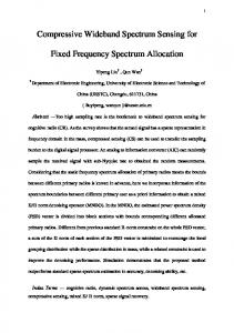
Figure 1. Block diagram of a Sub-Nyquist WSS system. Source: [9].

� 𝑘𝑘 = 𝒙𝒙

1 � 𝒙𝒙𝑛𝑛 𝜔𝜔𝑘𝑘𝑘𝑘 , 𝑘𝑘 ∈ [𝑁𝑁] 𝑁𝑁

(1)

sensing techniques use preambles and pilot signals. However, these sensing techniques are narrowband because they can only sense a single carrier frequency. On the one hand, measurements carried out by the Microsoft Spectrum Observatory at Washington DC [4] show that around 3% of the band between 30 MHz and 3 GHz is used sparsely to host most of the worldwide radio services [4]. This sparse occupancy of the radio electric spectrum has motivated the theoretical research about Wideband Spectrum Sensing (WSS) techniques during the last five years [5-7]. In this case, the research results have shown that sub-Nyquist sampling techniques such as Analog to Information Conversion (AIC) [6],[8], Modulated Wideband Conversion (MWC) [6][10] and Multi Coset (MC) sampling [6],11,12] are promissory candidates for developing WSS systems as the shown in Fig. 1 The sub-Nyquist WSS systems are usually composed of a sub-Nyquist sampler, a spectral reconstruction block and a decision stage [5,6[9]. The spectral reconstruction block is usually constructed by using Compressive Sensing (CS) techniques [13,14]. On the other hand, spectral reconstruction considering the Sparse Fast Fourier Transform (sFFT) algorithms [15-19] has not been well developed as these algorithms either require a high sampling cost for typical spectrum occupancy [15,16,[19], they are very noise sensitive [17], or they are too complex [18]. In the context of WSS algorithms, the challenge is to achieve sub-Nyquist sampling rates using low-power and low-speed ADCs for highly-noisy signals. Thus, considering the above, the main contribution of this paper is the design of a new sub-Nyquist WSS algorithm that reduces the sampling cost by using a modified version of the sFFT algorithm with Gaussian small support windows. This proposed algorithm is very suitable for hardware implementation of WSS systems using ASICs or FPGAs, and to the best of our knowledge, it is the first that uses the recently developed Nearly Optimal Sparse Fourier Transform. The rest of the paper is organized as follows: Section 2 presents some mathematical basics about the sub-Nyquist WSS algorithm we developed, Section 3 describes the proposed sub-Nyquist WSS algorithm, Section 4 presents simulation results performed on scenarios composed of highly-noisy multiband-signals, and, Section 5, presents our conclusions and suggestions for future work.

� are the permuted spectrum signals in Where 𝒙𝒙𝒙𝒙 and 𝒙𝒙𝒙𝒙 the time domain and the DFT domain, respectively; 𝜋𝜋𝑝𝑝 (𝑘𝑘, 𝜎𝜎, 𝑁𝑁) = 𝜎𝜎𝜎𝜎 mod 𝑁𝑁 is the spectral permutation function; and 𝜎𝜎 ∈ {2𝑐𝑐 + 1|𝑐𝑐 ∈ [𝑁𝑁/2]} and 𝑎𝑎 ∈ [𝑁𝑁] are the spectral permutation parameters. The spectral permutation function translates the frequency bin from the 𝑘𝑘-th location to the 𝜋𝜋𝑝𝑝 (𝑘𝑘, 𝜎𝜎, 𝑁𝑁)-th location, in this case 𝜎𝜎 −1 mod 𝑁𝑁 exists for all odd 𝜎𝜎 if 𝑁𝑁 is a power of two. The sFFT algorithm randomly chooses the spectral permutation parameters 𝜎𝜎 and 𝑎𝑎 from a uniform distribution. Thus, the spectral permutation with these pseudo-random parameters is related to a pseudorandom sampling scheme [15-19].

2. Mathematical background

2.3. Filtering window

In this section, we present some fundamental concepts about the sub-Nyquist sFFT algorithm we developed. First,

The filtering window is a new mathematical tool that reduces the size of the FFT from points 𝑁𝑁 to 𝐵𝐵. This is accomplished in

𝑛𝑛∈[𝑁𝑁]

Where 𝑁𝑁 is a power of two, [𝑁𝑁] denotes the set of indexes { 0,1, … , 𝑁𝑁 − 1}, and 𝜔𝜔 = 𝑒𝑒 −i 2𝜋𝜋/𝑁𝑁 is the 𝑁𝑁-th root of unity. In this case, the number of non-zero elements of the � is called the sparsity order 𝐾𝐾 and is defined in Eq. (2). vector 𝒙𝒙

�)|0 𝐾𝐾 = |supp(𝒙𝒙

(2)

�) is the set of indexes of the non-zero Where supp(𝒙𝒙 �, and | |0 represents the 𝑙𝑙0 -norm of elements of the vector 𝒙𝒙 the vector. Then, a time domain signal 𝒙𝒙 is sparse in the DFT domain if 𝐾𝐾 ≪ 𝑁𝑁. In this context, a set of algorithms called sFFT takes advantage of the signal sparsity in the DFT domain to speed up the runtime of the Fast Fourier Transform (FFT) algorithms used to calculate the DFT [15-18]. These sFFT algorithms, like the Nearly Optimal sFFT algorithm presented in [16], use the following mathematical tools: pseudo-random spectral permutation [15-19], filtering window [16] and hashing function [15,16]. 2.2. Pseudo-random spectral permutation This permutation isolates spectral components from each other [19] and is performed as described in Eq. (3).

𝒙𝒙𝒑𝒑𝑛𝑛 = 𝒙𝒙𝜎𝜎(𝑛𝑛−𝑎𝑎)mod 𝑁𝑁 ,

� 𝜋𝜋𝑝𝑝 (𝑘𝑘,𝜎𝜎,𝑁𝑁) = 𝒙𝒙 �𝑘𝑘 𝜔𝜔𝜎𝜎𝜎𝜎𝜎𝜎 𝒙𝒙𝒙𝒙

80

(3)


sampled signal obtained from 𝒚𝒚. The vector that has the hashes � ∈ ℂ𝐵𝐵 and it is calculated using Eq. (9) [15,16]. of signal 𝒚𝒚 is 𝒖𝒖

the Nearly Optimal sFFT algorithm by extending a flat passband region of width 𝑁𝑁/𝐵𝐵 around each sparse component; this approach replaces the filter bank of previous sFFT algorithms [19,20] and avoids the use of non-equispaced data FFTs [21]. Nonetheless, this flat window has a support that is not small enough to achieve sub-Nyquist sampling rates. Thus, in order to reduce the sampling cost of the sFFT � ′ such algorithm, we designed a small support window 𝑮𝑮, 𝑮𝑮 that |supp(𝑮𝑮)|0 = 𝐵𝐵; nevertheless, this small support can reduce the accuracy, which is not a big issue in the case of WSS systems. In this case, the window in the time domain is designed with an ideal low-pass filter using a Gaussian window with finite duration to truncate the impulse response. The cutoff frequency of the low-pass filter is 2𝐶𝐶, where 𝐶𝐶 = 1/(2𝐵𝐵), and the standard deviation 𝜎𝜎𝑔𝑔 of the Gaussian window is obtained from the 68-95-99.7 rule [22], as described in Eq. (4).

𝜎𝜎𝑔𝑔 =

𝐵𝐵 6

� 𝒋𝒋 = 𝐷𝐷𝐷𝐷𝐷𝐷 � � 𝒚𝒚𝑗𝑗+𝐵𝐵𝐵𝐵 � , 𝑗𝑗 ∈ [𝐵𝐵] 𝒖𝒖

From Eq. (7)-(9), it is possible to note that for each sparse component of the signal 𝒙𝒙 there are 14 non-zero hashes located in the offsets given by Eqs. (10) and (11).

𝑜𝑜𝑓𝑓𝑓𝑓 (𝑗𝑗, 𝜎𝜎, 𝑁𝑁, 𝐵𝐵) = 𝜋𝜋𝑝𝑝 (𝑗𝑗, 𝜎𝜎, 𝑁𝑁) − (ℎ𝑓𝑓 (𝑗𝑗, 𝜎𝜎, 𝑁𝑁, 𝐵𝐵) − 𝑘𝑘)𝑁𝑁/𝐵𝐵, 𝑘𝑘 ∈ {0,1, … ,6} 𝑜𝑜𝑐𝑐𝑐𝑐 (𝑗𝑗, 𝜎𝜎, 𝑁𝑁, 𝐵𝐵) = 𝜋𝜋𝑝𝑝 (𝑗𝑗, 𝜎𝜎, 𝑁𝑁) − (ℎ𝑐𝑐 (𝑗𝑗, 𝜎𝜎, 𝑁𝑁, 𝐵𝐵) + 𝑘𝑘)𝑁𝑁/𝐵𝐵, 𝑘𝑘 ∈ {0,1, … ,6}

(4)

𝑮𝑮𝑛𝑛+𝑁𝑁mod 𝑁𝑁 = 2 𝐶𝐶 𝑒𝑒 2

sinc(2𝐶𝐶(𝑛𝑛

(5)

� 𝑁𝑁/2 , 𝑛𝑛 ∈ [𝑁𝑁] − 𝑁𝑁/2))/𝑮𝑮

�′ 𝑮𝑮

𝑁𝑁 𝑘𝑘+ mod 𝑁𝑁 2

=

0, if |𝑘𝑘 − 𝑁𝑁/2| ≥ 𝑁𝑁(𝐶𝐶 + 1/𝜎𝜎𝑔𝑔 )

⎧ 𝑁𝑁 𝑁𝑁 ⎪ ⎪ 𝑘𝑘 − 𝑘𝑘 − 2 + 𝐶𝐶�� − ncdf �2𝜋𝜋𝜎𝜎 � 2 − 𝐶𝐶�� ncdf �2𝜋𝜋𝜎𝜎𝑔𝑔 � 𝑔𝑔 , 𝑘𝑘 𝑁𝑁 𝑁𝑁 ⎨ ⎪ , otherwise ⎪ � 𝑁𝑁 𝑮𝑮 ⎩ 2 ∈ [𝑁𝑁]

(6)

(7)

Finally, the windowing process is described in Eq. (8), and it is performed in the time domain after the pseudorandom spectral permutation is carried out.

𝑦𝑦 = 𝑥𝑥𝑥𝑥 ∘ 𝐺𝐺

(11)

3. Sub-Nyquist wideband spectrum sensing algorithm

Where vector 𝑮𝑮′ is the approximated window and ncdf(𝑥𝑥) = erfc(−𝑥𝑥 / √2)/2 is the Normal Cumulative Distribution Function [23]. The Gaussian window is normalized both in the time domain and the DFT domain in order to achieve unit DC gain, and its total bandwidth in DFT domain is given by Eq. (7).

𝐵𝐵𝑊𝑊𝑮𝑮′ = 13𝑁𝑁/𝐵𝐵

(10)

Where ℎ𝑓𝑓 (𝑗𝑗, 𝜎𝜎, 𝑁𝑁, 𝐵𝐵) − 𝑘𝑘 mod 𝐵𝐵, 𝑘𝑘 ∈ {0,1, … ,6} and ℎ𝑐𝑐 (𝑗𝑗, 𝜎𝜎, 𝑁𝑁, 𝐵𝐵) + 𝑘𝑘 mod 𝐵𝐵, 𝑘𝑘 ∈ {0,1, … ,6} are the 14 indexes � for each hashed single sparse component, of the hashes 𝒖𝒖 and ℎ𝑓𝑓 (𝑗𝑗, 𝜎𝜎, 𝑁𝑁, 𝐵𝐵) = ⌊ 𝜋𝜋𝑝𝑝 (𝑗𝑗, 𝜎𝜎, 𝑁𝑁)𝐵𝐵/𝑁𝑁 ⌋ is the floor-hash function and ℎ𝑐𝑐 (𝑗𝑗, 𝜎𝜎, 𝑁𝑁, 𝐵𝐵) = ⌈𝜋𝜋𝑝𝑝 (𝑗𝑗, 𝜎𝜎, 𝑁𝑁)𝐵𝐵/𝑁𝑁⌉ is the ceilhash function. Finally, it has to be noted that the use of pseudo-random spectral permutation and small support windows leads to a sub-Nyquist random sampling scheme; where, under certain conditions, the average sampling rate is below Nyquist.

Eq. (5)-(6) describe the Gaussian window in the time domain and the DFT domain, respectively. (𝑛𝑛−𝑁𝑁/2)2 − 2𝜎𝜎𝑔𝑔2

(9)

𝑖𝑖∈[𝑁𝑁/𝐵𝐵]

(8)

Where, 𝒚𝒚 is the windowed signal in the time domain.

2.4. Hashing function

The hashing function obtains 𝐵𝐵 points from the 𝑁𝑁-point spectrum of the signal 𝒚𝒚, these points are separated by 𝑁𝑁/𝐵𝐵 bins, and they are obtained by calculating the 𝐵𝐵-point DFT of the sub-

81

In this section, we describe the Sub-Nyquist WSS algorithm, called SNSparseWSS, which presents a reduced sampling rate compared to the sFFT algorithm described in [16]. This improvement is achieved by using the window described in the past section and by performing several modifications to the procedures presented in [16]. The SNSparseWSS algorithm, described in Alg. 1, calculates the spectrum occupancy 𝑿𝑿𝑟𝑟𝑟𝑟𝑟𝑟𝑟𝑟 with constant False Alarm Probability (𝑃𝑃𝐹𝐹𝐹𝐹 ) [2],[11], and has the following input parameters: the sparse bandwidth 𝐵𝐵𝐵𝐵 in Hz, the total bandwidth 𝑊𝑊 in Hz, the duration of the sensing window 𝜏𝜏 in seconds, the noise power 𝜎𝜎𝑛𝑛 , and the constants of the sFFT algorithm 𝑅𝑅𝑒𝑒𝑒𝑒𝑒𝑒 and 𝑠𝑠 [16]. The algorithm calculates the spectrum occupancy using four processing stages: the first one performs sub-Nyquist sampling on the wideband complex signal 𝑥𝑥(𝑡𝑡); the second one locates the sparse components by using the vector 𝒙𝒙𝑙𝑙 , the set of permutation parameters 𝑷𝑷𝑙𝑙 , and the modified LocateSignal procedure [16],[24]; the third one estimates the DFT values by using the vector 𝒙𝒙𝑒𝑒 , the set of permutation parameters 𝑷𝑷𝑒𝑒 , and the modified EstimateValues procedure [15]; and the fourth one detects the occupied bands with constant 𝑃𝑃𝐹𝐹𝐹𝐹 using the ConstantPfaRecovery procedure, which determines whether a channel is occupied or not by a PU. Therefore, it is necessary to test two spectrum sensing hypotheses, 𝐻𝐻0 for vacant channel and 𝐻𝐻1 for occupied channel [2], by using a detector with constant 𝑃𝑃𝐹𝐹𝐹𝐹 [2],[11] as described in Eq. (12) [11].


Algorithm 1. SNSparseWSS algorithm.

𝑺𝑺𝑙𝑙 =

𝑺𝑺𝑒𝑒 =

�

(𝜎𝜎,𝑎𝑎,𝛽𝛽)∈𝑷𝑷𝒍𝒍 ,𝑛𝑛∈supp(G)

�

(𝜎𝜎,𝑎𝑎)∈𝑷𝑷𝒆𝒆 ,𝑛𝑛∈supp(G)

Input:

𝑁𝑁 2

� ∈ ℂ𝐵𝐵 Output: 𝒖𝒖

� ′� HashToBins procedure �𝒙𝒙 , 𝒛𝒛�, 𝐵𝐵, 𝜎𝜎, 𝑎𝑎, 𝑮𝑮, 𝑮𝑮 𝒖𝒖𝑗𝑗 = 0 ∀ 𝑗𝑗 ∈ [𝐵𝐵]; //Spectral permutation and sub-sampling for 𝑗𝑗 ∈ {𝑁𝑁 − |supp(𝑮𝑮)|0 /2, 𝑁𝑁 + |supp(𝑮𝑮)|0 /2 − 1} do 𝒖𝒖𝑗𝑗 mod 𝐵𝐵 = 𝒖𝒖𝑗𝑗 mod 𝐵𝐵 + 𝒙𝒙𝜎𝜎(𝑗𝑗−𝑎𝑎)mod 𝑁𝑁 𝑮𝑮𝑗𝑗−𝑁𝑁+|supp(𝑮𝑮)|0 /2 ; end //Sub-sampled DFT � = FFT𝐵𝐵 (𝒖𝒖); 𝒖𝒖 //Efficient convolution calculation for 𝑗𝑗 ∈ 𝑠𝑠𝑠𝑠𝑠𝑠𝑠𝑠(𝒛𝒛�) do for 𝑘𝑘 ∈ [6] do � ℎ𝑓𝑓 (𝑗𝑗,𝜎𝜎,𝑁𝑁,𝐵𝐵)−𝑘𝑘 mod 𝐵𝐵 = 𝒖𝒖 � ℎ𝑓𝑓 (𝑗𝑗,𝜎𝜎,𝑁𝑁,𝐵𝐵)−𝑘𝑘 mod 𝐵𝐵 𝒖𝒖 � ′�𝑜𝑜 (𝑗𝑗,𝜎𝜎,𝑁𝑁,𝐵𝐵)� 𝒛𝒛�𝑗𝑗 𝜔𝜔 𝜎𝜎𝜎𝜎𝜎𝜎 ; − 𝑮𝑮

𝜎𝜎(𝑛𝑛 − 𝑎𝑎 + 𝛽𝛽) mod 𝑁𝑁 ;

𝑓𝑓𝑓𝑓

𝜎𝜎(𝑛𝑛 − 𝑎𝑎) mod 𝑁𝑁 ;

𝐞𝐞𝐞𝐞𝐞𝐞

2

𝑿𝑿𝑟𝑟𝑟𝑟𝑟𝑟𝑟𝑟 = 𝑪𝑪𝑪𝑪𝑪𝑪𝑪𝑪𝑪𝑪𝑪𝑪𝑪𝑪𝑪𝑪𝑷𝑷𝒇𝒇𝒇𝒇 𝑹𝑹𝑹𝑹𝑹𝑹𝑹𝑹𝑹𝑹𝑹𝑹𝑹𝑹𝑹𝑹(𝑿𝑿𝑟𝑟 , 𝜎𝜎𝑛𝑛 , 𝑁𝑁, 𝑃𝑃𝐹𝐹𝐹𝐹 ); end return 𝑿𝑿𝑟𝑟𝑟𝑟𝑟𝑟𝑟𝑟 Source: Authors.

Where, 𝜓𝜓𝑗𝑗 = 𝜎𝜎2𝑛𝑛 ��

threshold.

2

𝑁𝑁3

𝑐𝑐𝑐𝑐

This procedure calculates the hashes-error using three processing stages: the first one simultaneously calculates in the time domain the pseudo-random spectral permutation, the windowing, and the hashing process; the second calculates � by performing the 𝐵𝐵-point FFT of the DFT domain hashes 𝒖𝒖 the time domain hashes 𝒖𝒖; and the third one calculates the hashes-error by subtracting the DFT domain hashes of 𝒛𝒛� from �, in this case there are 14 hashes for each sparse the hashes 𝒖𝒖 component in 𝒛𝒛�.

� 𝑱𝑱 �2 𝑿𝑿𝒓𝒓 =�𝒘𝒘

𝑿𝑿𝑟𝑟𝑗𝑗 ≥ 𝜓𝜓𝑗𝑗 otherwise

� ℎ𝑐𝑐(𝑗𝑗,𝜎𝜎,𝑁𝑁,𝐵𝐵)−𝑘𝑘 mod 𝐵𝐵 = 𝒖𝒖 � ℎ𝑐𝑐(𝑗𝑗,𝜎𝜎,𝑁𝑁,𝐵𝐵)−𝑘𝑘 mod 𝐵𝐵 𝒖𝒖 � ′|𝑜𝑜 (𝑗𝑗,𝜎𝜎,𝑁𝑁,𝐵𝐵)| 𝒛𝒛�𝑗𝑗 𝜔𝜔 𝜎𝜎𝜎𝜎𝜎𝜎 ; − 𝑮𝑮

end � return 𝒖𝒖 Source: Adapted from [16].

//Parallel random sampling of signal 𝒙𝒙𝑺𝑺𝑙𝑙 = 𝑥𝑥(𝑺𝑺𝑙𝑙 /𝑊𝑊); 𝒙𝒙𝑺𝑺𝑒𝑒 = 𝑥𝑥(𝑺𝑺𝑒𝑒 /𝑊𝑊); //sFFT calculation //Location of Components � ′, 𝑠𝑠, 𝑅𝑅𝑙𝑙𝑙𝑙𝑙𝑙 �; 𝑳𝑳 = 𝑳𝑳𝑳𝑳𝑳𝑳𝑳𝑳𝑳𝑳𝑳𝑳𝑳𝑳𝑳𝑳𝑳𝑳𝑳𝑳𝑳𝑳𝑳𝑳�𝒙𝒙𝑙𝑙 , 𝟎𝟎, 𝐵𝐵, 𝑷𝑷𝑙𝑙 , 𝑮𝑮, 𝑮𝑮 //Estimation of Components � ′, 𝑳𝑳, 3𝐾𝐾𝑟𝑟 , 𝑅𝑅𝑒𝑒𝑒𝑒𝑒𝑒 �; {𝒘𝒘 � , 𝑱𝑱} = 𝑬𝑬𝑬𝑬𝑬𝑬𝑬𝑬𝑬𝑬𝑬𝑬𝑬𝑬𝑬𝑬𝑬𝑬𝑬𝑬𝑬𝑬𝑬𝑬𝑬𝑬𝑬𝑬�𝒙𝒙𝒆𝒆 , 𝟎𝟎, 𝐵𝐵, 𝑷𝑷𝑒𝑒 , 𝑮𝑮, 𝑮𝑮

𝐻𝐻1 , 𝑿𝑿𝑟𝑟𝑟𝑟𝑟𝑟𝑟𝑟 𝑗𝑗 = � 𝐻𝐻0 ,

Algorithm 2. Modified Hash to bins function.

𝒙𝒙 ∈ ℂ𝑁𝑁 , 𝒛𝒛� ∈ ℂ𝑁𝑁 , 𝐵𝐵 ∈ {2𝑐𝑐 |𝑐𝑐 ∈ [log 2 𝑁𝑁]}, 𝜎𝜎 ∈ � ′ ∈ ℝ𝟏𝟏𝟏𝟏𝟏𝟏/𝑩𝑩 �2𝑐𝑐 + 1�𝑐𝑐 ∈ � �� , 𝑎𝑎 ∈ [𝑁𝑁], 𝑮𝑮 ∈ ℝ𝑩𝑩 , 𝑮𝑮

Input: Sparse bandwidth 𝐵𝐵𝐵𝐵 in Hz, total bandwidth 𝑊𝑊 in Hz, sensing time 𝜏𝜏 in seconds, number 𝑅𝑅𝑒𝑒𝑒𝑒𝑒𝑒 of estimation loops, threshold 𝑠𝑠 for location, noise power 𝜎𝜎𝑛𝑛 Output: 𝑿𝑿𝑟𝑟𝑟𝑟𝑟𝑟𝑟𝑟 SNSparseWSS 𝐩𝐩𝐩𝐩𝐩𝐩𝐩𝐩𝐩𝐩𝐩𝐩𝐩𝐩𝐩𝐩𝐩𝐩 (𝐵𝐵𝐵𝐵, 𝑊𝑊, 𝜏𝜏, 𝑅𝑅𝑒𝑒𝑒𝑒𝑒𝑒 , 𝑠𝑠, 𝜎𝜎𝑛𝑛 ) //Window generation 𝑁𝑁 = 2⌊log2 (𝑊𝑊×𝜏𝜏)⌋ ; 𝐾𝐾 = ⌈𝐵𝐵𝐵𝐵/𝑊𝑊 × 𝑁𝑁⌉; 𝐵𝐵 = 2⌊log2 𝐾𝐾⌋+1 ; 𝑅𝑅𝑙𝑙𝑙𝑙𝑙𝑙 = ⌊log 2 log 2 𝑁𝑁⌋; � ′) by using Eqs. (5) and (6). Calculate Gaussian Window (𝑮𝑮, 𝑮𝑮 //Sub-Nyquist sampling set genration Pre-calculate all permutation parameters in 𝑷𝑷𝑙𝑙 for 1 location loop [16]; Pre-calculate all permutation parameters in 𝑷𝑷𝑒𝑒 for 𝑅𝑅𝑒𝑒𝑒𝑒𝑒𝑒 estimation loops [16];

3.1.2. LocateSignal procedure

(12)

This procedure, presented in Alg. 3, calculates the set 𝑳𝑳 ∈ ℕ𝑂𝑂(𝐵𝐵) of frequency bins corresponding to 𝑂𝑂(𝐵𝐵) sparse components found in 𝒙𝒙; and it has the following input parameters: the time domain signal 𝒙𝒙; the instantaneous �; the parameter 𝐵𝐵; the spectral permutation estimation 𝒛𝒛� of 𝒙𝒙 � ′ of the filtering window in the parameters 𝑷𝑷𝑙𝑙 ; the vectors 𝑮𝑮, 𝑮𝑮 time domain and the DFT domain respectively; the threshold constant for location 𝑠𝑠 [16]; and the number of location iterations 𝑅𝑅𝑙𝑙𝑙𝑙𝑙𝑙 [16]. This procedure locates the sparse components of 𝒙𝒙 using four processing stages: the first one sets the initial conditions, the second one adjusts the frequency locations, the third one reduces the search region, and the fourth one inverts the spectral permutation. The setting of initial conditions is �; performed by first calculating a reference hashes vector 𝒖𝒖 (0) second pre-calculating an initial guess of value 𝒍𝒍𝑗𝑗 = 𝑗𝑗𝑗𝑗/𝐵𝐵 ∀ ~ 𝑗𝑗 ∈ [𝐵𝐵] of frequency locations in the permuted spectrum; and third by pre-calculating the initial values of 𝑤𝑤, 𝑡𝑡, and 𝐷𝐷𝑚𝑚𝑚𝑚𝑚𝑚 , where 𝑤𝑤 is the width of the region for searching the frequency adjustment, 𝑡𝑡 is the number of candidate adjustments in 𝑤𝑤, 𝐷𝐷𝑚𝑚𝑚𝑚𝑚𝑚 is the number of

𝑄𝑄−1 (𝑃𝑃𝐹𝐹𝐹𝐹 ) + 1/𝑁𝑁� is the decision

3.1. Modified procedures We modified the HashToBins, LocateSignal, LocateInner, and EstimateValues procedures described in [16] in order to use the proposed filtering window and to reduce the execution time. 3.1.1. HashToBins procedure This procedure, presented in Alg. 2, calculates the hasheserror by subtracting the hashes of the instantaneous estimation 𝒛𝒛� � [16], and it has the following input from the hashes 𝒖𝒖 parameters: the time domain signal 𝒙𝒙; the instantaneous �; the parameter 𝐵𝐵; the spectral permutation estimation 𝒛𝒛� of 𝒙𝒙 � ′ of the filtering window parameters 𝜎𝜎, and 𝑎𝑎; and the vectors 𝑮𝑮, 𝑮𝑮 in the time domain and the DFT domain respectively. 82


Algorithm 3. Modified locate signal function.

Input: 𝒙𝒙 ∈ ℂ𝑂𝑂(𝐾𝐾) , 𝒛𝒛� ∈ ℂ𝑁𝑁 , 𝐵𝐵 ∈ {2𝑐𝑐 |𝑐𝑐 ∈ [log 2 𝑁𝑁]}, 𝑷𝑷𝑙𝑙 ∈ ℕ3×𝑂𝑂(𝐾𝐾) , 𝑮𝑮 ∈

Input:

𝟏𝟏𝟏𝟏𝟏𝟏 𝑩𝑩

2

� ∈ ℂ𝐵𝐵 , 𝒍𝒍 ∈ ℕ𝑂𝑂(𝐵𝐵) ℝ, 𝑡𝑡 ∈ ℕ+ , 𝒖𝒖 Output: 𝒍𝒍′ ∈ ℕ𝑂𝑂(𝐵𝐵)

= 𝑗𝑗𝑗𝑗/𝐵𝐵 ∀ ~ 𝑗𝑗 ∈ [𝐵𝐵];

(𝐷𝐷𝑚𝑚𝑚𝑚𝑚𝑚 )

+ 0.5 � �𝑗𝑗 ∈ [𝐵𝐵]� ;

return 𝑳𝑳 Source: Adapted from [16].

𝑁𝑁

adjustments, and 𝑅𝑅𝑙𝑙𝑙𝑙𝑙𝑙 is the number of location iterations for each adjustment. The adjustment of frequency locations is performed by using 𝐷𝐷𝑚𝑚𝑚𝑚𝑚𝑚 times the procedure LocateInner. The reduction of the search region is performed by dividing 𝑤𝑤 by a factor 1/(𝑡𝑡 ′ )𝐷𝐷 at the 𝐷𝐷-th adjustment, this reduction allows a systematic refining of the frequency location. Finally, the spectral permutation inversion is performed by calculating the function 𝜋𝜋−1 𝑝𝑝 (𝑘𝑘, 𝜎𝜎, 𝑁𝑁) on each located frequency.

end

if min {�𝜃𝜃𝑗𝑗,𝑞𝑞 − 𝑐𝑐𝑗𝑗 �, 2𝜋𝜋 − �𝜃𝜃𝑗𝑗,𝑞𝑞 − 𝑐𝑐𝑗𝑗 �} < 𝑠𝑠𝑠𝑠 then 𝒗𝒗𝑗𝑗,𝑞𝑞 = 𝒗𝒗𝑗𝑗,𝑞𝑞 + 1; end

end end end for 𝑗𝑗 ∈ [𝐵𝐵] do 𝑸𝑸 = �𝑞𝑞 ∈ [𝑡𝑡] �𝒗𝒗𝑗𝑗,𝑞𝑞 > 𝑅𝑅𝑙𝑙𝑙𝑙𝑙𝑙 /2�; if 𝑸𝑸 ≠ ∅ then 𝒍𝒍𝑗𝑗′ = 𝒍𝒍𝑗𝑗 + min 𝑞𝑞𝑞𝑞/𝑡𝑡;

3.1.3. LocateInner procedure

This procedure, presented in Alg. 4, calculates the adjustment 𝒍𝒍′ ∈ ℕ𝑂𝑂(𝐵𝐵) of the frequency locations in the permuted spectrum, and it has the following input parameters: �; the time domain signal 𝒙𝒙; the instantaneous estimation 𝒛𝒛� of 𝒙𝒙 the parameter 𝐵𝐵; the spectral permutation parameters 𝜎𝜎, 𝑎𝑎, and � ′ of the filtering window in the time domain 𝑷𝑷𝑙𝑙 ; the vectors 𝑮𝑮, 𝑮𝑮 and the DFT domain respectively; the threshold constant for location 𝑠𝑠; the number of location iterations 𝑅𝑅𝑙𝑙𝑙𝑙𝑙𝑙 ; the width of search region 𝑤𝑤; the number of candidate adjustments 𝑡𝑡; the �; and the current estimation of reference hashes vector 𝒖𝒖 frequency locations 𝒍𝒍. This procedure performs the adjustment of the frequency location using five processing stages: the first one sets the initial conditions, the second calculates the hashes-error, the third calculates the angles of the hashes-error and candidate frequency bins, the fourth performs the voting stage, and the fifth locates the frequency bins. The setting of initial conditions clears the vote counters of the 𝑡𝑡 candidate adjustments for the 𝐵𝐵 candidate frequency bins. The hashes �′, which are calculation stage obtains 𝑅𝑅𝑙𝑙𝑙𝑙𝑙𝑙 hashes vectors 𝒖𝒖 calculated from the signal 𝒙𝒙 by using the HashToBins procedure with pseudo-random permutation parameters of the form (𝜎𝜎, 𝑎𝑎 + 𝛽𝛽). The angle calculation stage obtains the vector 𝒄𝒄, which represents the angle differences between the � and the hashes 𝒖𝒖 �′. The voting stage reference hashes 𝒖𝒖 increments the vote counter 𝒗𝒗𝑗𝑗,𝑞𝑞 corresponding

, 𝑠𝑠 ∈ ℝ, 𝑅𝑅𝑙𝑙𝑙𝑙𝑙𝑙 ∈ ℕ+ , 𝑤𝑤 ∈

� ′, 𝑠𝑠, 𝑅𝑅𝑙𝑙𝑙𝑙𝑙𝑙 𝑤𝑤, 𝑡𝑡, 𝒖𝒖 �, 𝒍𝒍� LocateInner procedure �𝒙𝒙 , 𝒛𝒛�, 𝐵𝐵, 𝜎𝜎, 𝑎𝑎, 𝑷𝑷𝑙𝑙 , 𝑮𝑮, 𝑮𝑮 𝒗𝒗𝑗𝑗,𝑞𝑞 = 0 ∀ (𝑗𝑗, 𝑞𝑞) ∈ [𝐵𝐵] × [𝑡𝑡]; //Main loop for 𝑖𝑖 ∈ [𝑅𝑅𝑙𝑙𝑙𝑙𝑙𝑙 ] do Choose 𝛽𝛽 from 𝑷𝑷𝑙𝑙 ; � ′�; �′ =HashToBins�𝒙𝒙 , 𝒛𝒛�, 𝐵𝐵, 𝜎𝜎, 𝑎𝑎 + 𝛽𝛽, 𝑮𝑮, 𝑮𝑮 𝒖𝒖 for 𝑗𝑗 ∈ [𝐵𝐵] do if 𝒍𝒍𝑗𝑗 ≠ ⊥ then �𝑗𝑗 /𝒖𝒖 �𝑗𝑗′ ; 𝑟𝑟𝑗𝑗 = 𝒖𝒖 𝑐𝑐𝑗𝑗 = arctan2(ℑ{𝑟𝑟𝑗𝑗 }, ℜ{𝑟𝑟𝑗𝑗 }); if 𝑐𝑐𝑗𝑗 < 0 then 𝑐𝑐𝑗𝑗 = 𝑐𝑐𝑗𝑗 + 2𝜋𝜋; end for 𝑞𝑞 ∈ [𝑡𝑡] do 𝑞𝑞 + 1/2 𝑤𝑤; 𝑚𝑚𝑗𝑗,𝑞𝑞 = 𝒍𝒍𝑗𝑗 + 𝑡𝑡 2𝜋𝜋𝜋𝜋𝑚𝑚𝑗𝑗,𝑞𝑞 𝜃𝜃𝑗𝑗,𝑞𝑞 = mod 2𝜋𝜋;

𝑤𝑤0 = 𝑁𝑁/𝐵𝐵; 𝑡𝑡 = log 2 𝑁𝑁 ; 𝑡𝑡′ = 𝑡𝑡/4; 𝐷𝐷𝑚𝑚𝑚𝑚𝑚𝑚 = ⌈ log 𝑡𝑡 ′ (𝑤𝑤0 + 1)⌉; //Main loop for 𝐷𝐷 ∈ [𝐷𝐷𝑚𝑚𝑚𝑚𝑚𝑚 ] do � ′, 𝑠𝑠, 𝑅𝑅𝑙𝑙𝑙𝑙𝑙𝑙 , 𝑤𝑤0 𝒍𝒍(𝐷𝐷+1) = 𝑳𝑳𝑳𝑳𝑳𝑳𝑳𝑳𝑳𝑳𝑳𝑳𝑳𝑳𝑳𝑳𝑳𝑳𝑳𝑳𝑳𝑳(𝒙𝒙 , 𝒛𝒛�, 𝐵𝐵, 𝜎𝜎, 𝑎𝑎, 𝑷𝑷𝑙𝑙 , 𝑮𝑮, 𝑮𝑮 �, 𝒍𝒍(𝐷𝐷) ); /(𝑡𝑡 ′ )𝐷𝐷 , 𝑡𝑡, 𝒖𝒖 end 𝑳𝑳 = �𝜎𝜎 −1 � 𝒍𝒍𝑗𝑗

𝟏𝟏𝟏𝟏𝟏𝟏 𝑩𝑩

�′ ∈ ℝ �2𝑐𝑐 + 1�𝑐𝑐 ∈ � �� , 𝑎𝑎 ∈ [𝑁𝑁], 𝑮𝑮 ∈ ℝ𝑩𝑩 , 𝑮𝑮

� ′, 𝑠𝑠, 𝑅𝑅𝑙𝑙𝑙𝑙𝑙𝑙 � LocateSignal 𝐩𝐩𝐩𝐩𝐩𝐩𝐩𝐩𝐩𝐩𝐩𝐩𝐩𝐩𝐩𝐩𝐩𝐩 �𝒙𝒙, 𝒛𝒛�, 𝐵𝐵, 𝑷𝑷𝑙𝑙 , 𝑮𝑮, 𝑮𝑮 Choose 𝑎𝑎 and 𝜎𝜎 from 𝑷𝑷𝑙𝑙 ; � ′� � =HashToBins�𝒙𝒙 , 𝒛𝒛�, 𝐵𝐵, 𝜎𝜎, 𝑎𝑎, 𝑮𝑮, 𝑮𝑮 𝒖𝒖 (0)

𝒙𝒙 ∈ ℂ𝑁𝑁 , 𝒛𝒛� ∈ ℂ𝑁𝑁 , 𝐵𝐵 ∈ {2𝑐𝑐 |𝑐𝑐 ∈ [log 2 𝑁𝑁]}, 𝜎𝜎 ∈

𝑁𝑁

� ′ ∈ ℝ , 𝑠𝑠 ∈ ℝ, 𝑅𝑅𝑙𝑙𝑙𝑙𝑙𝑙 ∈ ℕ ℝ𝑩𝑩 , 𝑮𝑮 Output: 𝑳𝑳 ∈ ℕ𝑂𝑂(𝐵𝐵)

𝒍𝒍𝑗𝑗

Algorithm 4. Modified locate signal inner function.

else

𝒍𝒍𝑗𝑗′ =⊥;

𝑞𝑞∈𝑸𝑸

end end return 𝒍𝒍′ Source: Adapted from [16].

to the 𝑗𝑗-th frequency bin and 𝑞𝑞-th adjustment, if Eq. (13) is satisfied. min {�𝜃𝜃𝑗𝑗,𝑞𝑞 − 𝑐𝑐𝑗𝑗 �, 2𝜋𝜋 − �𝜃𝜃𝑗𝑗,𝑞𝑞 − 𝑐𝑐𝑗𝑗 �} < 𝑠𝑠𝑠𝑠

(13)

Where 𝜃𝜃𝑗𝑗,𝑞𝑞 is the angle of the 𝑗𝑗-th candidate frequency bin for the 𝑞𝑞-th adjustment, that is, 𝜃𝜃𝑗𝑗,𝑞𝑞 is related to the 𝑞𝑞-th candidate frequency adjustment 𝑞𝑞𝑞𝑞/𝑡𝑡. Additionally, the above calculation converges if 𝛽𝛽 is chosen at random from the set {⌊𝑠𝑠𝑠𝑠𝑠𝑠/ 4𝑤𝑤⌋, … , ⌊𝑠𝑠𝑠𝑠𝑠𝑠/2𝑤𝑤⌋} with enough small threshold 𝑠𝑠. Finally, the frequency location stage selects the minimum 𝑞𝑞 from the set 𝑸𝑸 = �𝑞𝑞 ∈ [𝑡𝑡] �𝑣𝑣𝑗𝑗,𝑞𝑞 > 𝑅𝑅𝑙𝑙𝑙𝑙𝑙𝑙 /2�; thus the estimated 𝑗𝑗-th permutedfrequency bin is refined using Eq. (14). 𝒍𝒍𝑗𝑗′ = 𝒍𝒍𝑗𝑗 + min 𝑞𝑞𝑞𝑞/𝑡𝑡 𝑞𝑞∈𝑸𝑸

83

(14)


Input:

Algorithm 5. Modified estimate values function.

𝒙𝒙 ∈ ℂ𝑁𝑁 , 𝒛𝒛� ∈ ℂ𝑁𝑁 , 𝐵𝐵 ∈ {2𝑐𝑐 |𝑐𝑐 ∈ [log 2 𝑁𝑁]}, 𝑷𝑷𝑒𝑒 ∈ ℕ2×𝑂𝑂(𝐾𝐾) , 𝑮𝑮 ∈

𝟏𝟏𝟏𝟏𝟏𝟏 𝑩𝑩

� ′ ∈ ℝ , 𝑳𝑳 ∈ ℕ𝑂𝑂(𝐵𝐵) , 𝐾𝐾 ′ ∈ ℕ+ , 𝑅𝑅𝑒𝑒𝑒𝑒𝑒𝑒 ∈ ℕ+ ℝ𝑩𝑩 , 𝑮𝑮 Output: 𝑳𝑳 ∈ ℕ𝑂𝑂(𝐵𝐵) � ′, 𝑳𝑳, 𝐾𝐾 ′ , 𝑅𝑅𝑒𝑒𝑒𝑒𝑒𝑒 � EstimateValues 𝐩𝐩𝐩𝐩𝐩𝐩𝐩𝐩𝐩𝐩𝐩𝐩𝐩𝐩𝐩𝐩𝐩𝐩 �𝒙𝒙 , 𝒛𝒛�, 𝐵𝐵, 𝑮𝑮, 𝑮𝑮

𝒘𝒘 �𝑗𝑗 = 0 ∀ 𝑗𝑗 ∈ [|𝑳𝑳|0 ]; //Main loop for 𝑖𝑖 ∈ [𝑅𝑅𝑒𝑒𝑒𝑒𝑒𝑒 ] do Choose 𝜎𝜎𝑖𝑖 and 𝑎𝑎𝑖𝑖 from 𝑷𝑷𝑒𝑒 ; � ′�; � =HashToBins�𝒙𝒙 , 𝒛𝒛�, 𝐵𝐵, 𝜎𝜎𝑖𝑖 , 𝑎𝑎𝑖𝑖 , 𝑮𝑮, 𝑮𝑮 𝒖𝒖 for 𝑗𝑗 ∈ [|𝑳𝑳|0 ] do �′ � ′𝑖𝑖,𝑗𝑗 = 𝒖𝒖 � ℎ�𝑳𝑳𝑗𝑗 ,𝜎𝜎𝑖𝑖,𝑁𝑁,𝐵𝐵�mod 𝑩𝑩 𝜔𝜔 −𝜎𝜎𝑖𝑖𝑎𝑎𝑖𝑖𝑳𝑳𝑗𝑗 /𝑮𝑮 𝒖𝒖 |𝑜𝑜�𝑳𝑳𝑗𝑗 ,𝜎𝜎𝑖𝑖 ,𝑁𝑁,𝐵𝐵�| ;

end end for 𝑗𝑗 ∈ [|𝑳𝑳|0 ] do // Median for real and imaginary separately across the i dimension ′ � 𝑖𝑖,𝑗𝑗 𝒘𝒘 �𝑗𝑗 = median𝑖𝑖 𝒖𝒖 end �𝒘𝒘 � 𝑱𝑱 �2 𝑱𝑱 = arg max

parts

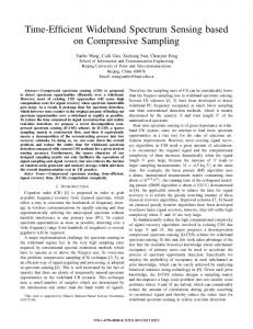
Figure 2. Percent of Nyquist Sampling Rate versus Spectrum occupancy percent for SNSparseWSS algorithm. Source: Authors.

|𝑱𝑱|0 =min{|𝑳𝑳|0 ,𝐾𝐾′}

𝑺𝑺 =

return {𝒘𝒘 � 𝑱𝑱 , 𝑱𝑱} Source: Adapted from [16].

�

𝑛𝑛 ∈ supp(𝑮𝑮)

��𝜎𝜎𝑖𝑖 (𝑛𝑛 − 𝑎𝑎𝑖𝑖 )� mod 𝑁𝑁�

(15)

Considering the set of sampling points 𝑺𝑺, it is possible to calculate the average sampling rate 𝑓𝑓𝑠𝑠𝑠𝑠 of the SNSparseWSS algorithm using Eq. (16).

3.1.4. EstimateValues procedure This procedure, presented in Alg. 5, calculates the DFT � 𝑱𝑱 , and it has the following input estimation adjustment 𝒘𝒘 parameters: the time domain signal 𝒙𝒙; the instantaneous �; the parameter 𝐵𝐵; the spectral permutation estimation 𝒛𝒛� of 𝒙𝒙 � ′ of the filtering window in parameters 𝑷𝑷𝑒𝑒 ; the vectors 𝑮𝑮, 𝑮𝑮 the time domain and the DFT domain respectively; the set of located sparse components 𝑳𝑳; the number of sparse components to estimate 𝐾𝐾′; and the number of estimation iterations 𝑅𝑅𝑒𝑒𝑒𝑒𝑒𝑒 [16]. This procedure calculates the DFT � 𝑱𝑱 using three processing stages: the estimation adjustment 𝒘𝒘 first one calculates the 𝑅𝑅𝑒𝑒𝑒𝑒𝑒𝑒 sets of hashes-error from the signal 𝒙𝒙 by using the HashToBins procedure and considering different pseudo-random permutation parameters; the second one separately calculates the median of the real and imaginary parts of the calculated hashes-error by only considering the set of located sparse frequency bins in 𝑳𝑳, and by cancelling the pseudo-random spectral permutation and the effect of the windowing in the DFT domain; and the third � 𝑱𝑱 . one saves the 𝐾𝐾′ most energetic components 𝒘𝒘

𝑓𝑓𝑠𝑠𝑠𝑠 = 𝑓𝑓𝑁𝑁𝑁𝑁𝑁𝑁

|𝑺𝑺|0 ∑𝑘𝑘∈supp(𝑺𝑺) 𝛻𝛻𝑺𝑺𝑘𝑘

(16)

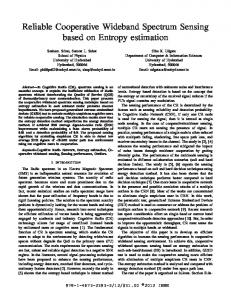
Where, 𝑓𝑓𝑁𝑁𝑁𝑁𝑁𝑁 is the Nyquist frequency, and 𝛻𝛻𝑺𝑺𝑘𝑘 = 𝑺𝑺𝑘𝑘 − 𝑺𝑺𝑘𝑘−1 is a finite-backward difference to estimate the average separation between samples. Fig. 2 shows the percentage of Nyquist frequency versus the percentage of spectrum occupancy for the SNSparseWSS algorithm. From Fig. 2, we can see that the algorithm reaches a sampling rate of close to 0.6 × 𝑓𝑓𝑁𝑁𝑁𝑁𝑁𝑁 for a spectrum occupancy between 2% and 3%; thus, for typical scenarios where the spectrum occupancy is close to 2% the SNSparseWSS algorithm is very suitable for implementing sub-Nyquist WSS systems and its performance is comparable to the WSS systems based on MC sampling [11]. 4.2. Verification of the SNSparseWSS algorithm In order to verify the WSS capabilities of the SNSparseWSS algorithm, we considered as test vehicle a highly-noisy multiband-signal scenario composed of 5 time domain signals located in the center frequencies 317-5761300-984-163 MHz, and a total bandwidth 𝑊𝑊 of 1.5 GHz. Each signal has a bandwidth of 5 MHz, is composed of random 4-QAM symbols that are filtered using a raised cosine filter with roll-off factor r = 0.5, and has SNR values from -5 dB to 5 dB. The test signal with SNR=-5 dB is shown in Fig. 3.

4. Simulation results of SNSparseWSS algorithm

This section presents the simulation results of the SNSparseWSS algorithm for sub-Nyquist sampling and verification results for Wideband Spectrum Sensing. 4.1. Sub-Nyquist capabilities In order to verify the sampling cost, we need to know all the spectral permutation parameters 𝜎𝜎𝑖𝑖 and 𝑎𝑎𝑖𝑖 that are pseudo-randomly generated by the SNSparseWSS algorithm; thus, the set of sampling points can be calculated using Eq. (15). 84


Figure 3. Wideband spectrum of 1.5 GHz containing 5 signals each with bandwidth 𝑩𝑩𝑩𝑩 = 5 MHz and SNR = -5 dB. Source: Authors.

Figure 5. Wideband spectrum sensing result by using the constant false alarm probability detector. Source: Authors.

In this case, the duration of the spectrum sensing window is 𝜏𝜏 = 160 𝜇𝜇𝜇𝜇 which implies that an FFT with 𝑁𝑁 = 217 must be used, and the total sparse bandwidth is 25 MHz (5 signals × 5 MHz) which leads to a sub-sampled FFT with 𝐵𝐵 = 8192. The algorithm was parameterized with 𝑅𝑅𝑒𝑒𝑒𝑒𝑒𝑒 = 10 estimation iterations and a location threshold of 𝑠𝑠 = 0.1, with these settings the SNSparseWSS algorithm achieves an average sampling rate of 𝑓𝑓𝑠𝑠𝑠𝑠 = 0.599 × 𝑓𝑓𝑁𝑁𝑁𝑁𝑁𝑁 . Fig. 4 shows the recovered spectrum using the SNSparseWSS algorithm. In this figure, we can see that the Gaussian small support window increases the total error of estimated DFT value; this issue can be mitigated using appropriate settings for the constant 𝑃𝑃𝐹𝐹𝐹𝐹 detector, which implies that the occupied channels can be detected with constant 𝑃𝑃𝐹𝐹𝐹𝐹 [11]. Fig. 5 shows the WSS simulation results using the constant 𝑃𝑃𝐹𝐹𝐹𝐹 detector with 𝑃𝑃𝐹𝐹𝐹𝐹 = 0.01. In this figure, we can see that the algorithm can perform WSS by detecting the occupied channels by the Pus. If additional information about the multiband-signal is available, such as the minimum channel separation 𝛥𝛥𝑓𝑓 [11], the detection can be improved by reducing the 𝑃𝑃𝐹𝐹𝐹𝐹 .

Figure 6. False alarm probability performance for different SNRs. Source: Authors.

Fig. 6 shows simulation results for the false alarm probability with SNR values of -5 dB, -2.5 dB, 0 dB, 2.5 dB, and 5 dB. In this figure we can see that the 𝑃𝑃𝐹𝐹𝐹𝐹 is approximately constant regardless the SNR of the multibandsignals. 5. Conclusions and future work In this paper, we present the design of a novel algorithm for sub-Nyquist Wideband Spectrum Sensing based on a modified Nearly Optimal sFFT algorithm. This WSS algorithm was verified using several tests. From the verification results we can conclude that the proposed algorithm is suitable for implementing the spectrum sensing function of wideband cognitive radios in highly-noisy environments. To the best of our knowledge, the proposed WSS algorithm is the first that uses the new Nearly Optimal Sparse Fourier Transform algorithm, and it has a reduced sampling cost by using flat Gaussian small support windows

Figure 4. Recovered spectrum for 𝜏𝜏 = 160 𝜇𝜇𝜇𝜇 (𝑁𝑁 = 217 ) 𝐵𝐵 = 8192, , 1 location iteration, 10 estimation iterations, and Gaussian window with |supp(𝑮𝑮)|0 = 𝐵𝐵. Source: Authors. 85


and modified procedures. Future work will addressed efficient hardware implementation of the modified Nearly Optimal sFFT algorithm using an FPGA.

[17]

Acknowledgements

[18]

Alexander López Parrado thanks Colciencias for the scholarship, and he also thanks Universidad del Quindío for the study commission.

[19]

References

[20]

[1]

[21]

[2]

[3]

[4]

[5]

[6]

[7]

[8]

[9]

[10]

[11]

[12] [13]

[14]

[15]

[16]

Mitola, J. and Maguire, G.Q., Cognitive radio: Making software radios more personal. IEEE Personal Communications, 6(4), pp. 1318, 1999. DOI: 10.1109/98.788210. Arslan, H., Cognitive radio, software defined radio, and adaptive wireless systems. Dordrecht: Springer, 2007. DOI: 10.1007/978-14020-5542-3. IEEE. IEEE 802.22-2011, wireless regional area networks (wran) – specific requirements part 22: Cognitive wireless ran medium access control (mac) and physical layer (phy) specifications: Policies and procedures for operation in the tv bands. 2011. DOI: 10.1109/IEEESTD.2011.5951707. M.T.P. Group, Microsoft spectrum observatory, [online], Seattle, [Date of reference, Nov. 2013.]. Available at: http://spectrumobservatory.cloudapp.net/. Vito, L.D., A review of wideband spectrum sensing methods for cognitive radios, Proceedings of Instrumentation and Measurement Technology Conference (I2MTC), pp. 2257-2262, 2012. DOI: 10.1109/I2MTC.2012.6229530. Hongjian, S., Nallanathan, A., Wang, C.X. and Chen, Y., Wideband spectrum sensing for cognitive radio networks: a survey. IEEE Wireless Communications, 20(2), pp. 74-81, 2013. DOI: 10.1109/MWC.2013.6507397. Axell, E., Leus, G., Larsson, E.G. and Poor, H.V., Spectrum sensing for cognitive radio: State-of-the-art and recent advances. IEEE Signal Processing Magazine, 29(3), pp. 101-116, 2012. DOI: 10.1109/MSP.2012.2183771. Laska, J., Kirolos, S., Duarte, M., Ragheb, T., Baraniuk, R. and Massoud, Y., Theory and implementation of an analog-to-information converter using random demodulation, Proceedings of IEEE International Symposium on Circuits and Systems, pp. 1959-1962, 2007. DOI: 10.1109/ISCAS.2007.378360. Sun, H., Chiu, W.Y., Jiang, J., Nallanathan, A. and Poor, H.V., Wideband spectrum sensing with Sub-Nyquist sampling in cognitive radios. IEEE Transactions on Signal Processing, 60(11), pp. 60686073, 2012. DOI: 10.1109/TSP.2012.2212892. Mishali, M. and Eldar, Y.C., From theory to practice: Sub-nyquist sampling of sparse wideband analog signals. IEEE Journal of Selected Topics in Signal Processing, 4(2), pp. 375-391, 2010. DOI: 10.1109/JSTSP.2010.2042414. Yen, C.-P., Tsai, Y. and Wang, X., Wideband spectrum sensing based on Sub-Nyquist sampling. IEEE Transactions on Signal Processing, 61(12), pp. 3028-3040, 2013. DOI: 10.1109/TSP.2013.2251342. Tsui, J.B., Digital techniques for wideband receivers, 2nd Edition. Raleigh: Scitech, 2004. DOI: 10.1049/SBRA005E. Donoho, D.L., Compressed sensing. IEEE Transactions on Information Theory, 52(4), pp. 1289-1306, 2006. DOI: 10.1109/TIT.2006.871582. Lobato-Polo, A.P., Ruiz-Coral, R.H., Quiroga-Sepúlveda, J.A. and Recio-Vélez, A.L., Sparse signal recovery using orthogonal matching pursuit (OMP). Ingeniería e Investigación, 29(2), pp. 112-118, 2009. Hassanieh, H., Indyk, P., Katabi, D. and Price, E., Simple and practical algorithm for sparse fourier transform, Proceedings of ACM-SIAM Symposium on Discrete Algorithms (SODA), pp. 11831194, 2012. DOI: 10.1137/1.9781611973099.93. Hassanieh, H., Indyk, P., Katabi, D. and Price, E., Nearly optimal sparse fourier transform, Proceedings of the 44th symposium on

[22] [23]

[24]

Theory of Computing (STOC), pp. 563-578, 2012. DOI: 10.1145/2213977.2214029. Hassanieh, H., Shi, L., Abari, O., Hamed, E. and Katabi, D., Ghz-wide sensing and decoding using the sparse fourier transform, Proceedings of IEEE INFOCOM, pp. 2256-2264, 2014. DOI: 10.1109/INFOCOM.2014.6848169. Indyk , P., Kapralov, M. and Price, E., (Nearly) Sample-optimal sparse fourier transform, Proceedings of ACM-SIAM Symposium on Discrete Algorithms (SODA), pp. 480-499, 2014. DOI: 10.1137/1.9781611973402.36. Gilbert, A.C., Strauss, M.J. and Tropp, J.A., A tutorial on fast fourier sampling. IEEE Signal Processing Magazine, 25(2), pp. 57-66, 2008. DOI: 10.1109/MSP.2007.915000. Gilbert, A.C., Muthukrishnan, S. and Strauss, M.J., Improved time bounds for near-optimal sparse fourier representations, Proceedings of SPIE Wavelets XI, pp. 1-15, 2005. DOI: 10.1117/12.615931. Dutt, A. and Rokhlin, V., Fast fourier transforms for nonequispaced data, ii. Applied and Computational Harmonic Analysis, 2(1), pp. 85100, 1995. DOI: 10.1006/acha.1995.1007. Tanton, J., Encyclopedia of Mathematics. New York: Facts on File, 2005. Abramowitz, M. and Stegun, I., Handbook of mathematical functions with formulas, graphs, and mathematical tables, 10th printing. Washington, D.C.: Dover, 1972. DOI: 10.1063/1.3047921. Gilbert, A.C., Li, Y., Porat, E. and Strauss, M.J., Approximate sparse recovery: Optimizing time and measurements, Proceedings of the 42nd ACM symposium on Theory of computing, pp. 475-484, 2010. DOI: 10.1145/1806689.1806755.

A. López-Parrado, completed his BSc. Eng. in Electronics Engineering in 2002 at Universidad del Quindío, Armenia, Colombia, and his MSc. degree in Electronics in 2009 at Universidad del Valle, Cali, Colombia. He is currently a PhD. candidate in Electrical and Electronics Engineering at Universidad del Valle, Cali, Colombia. His research interests are the FPGA design of complex digital systems, design of baseband processors, DSP complex functions, embedded systems, and compressive sensing. He is an assistant professor in the Electronics Engineering Program at Universidad del Quindío, Colombia. ORCID: 0000-0002-0274-6901 J. Velasco-Medina, completed his BSc. Eng. in Electrical Engineering in 1985 at Universidad del Valle, Cali, Colombia, his MSc. degree in Microelectronics 1995 at Universite De Grenoble I (Scientifique Et Medicale - Joseph Fourier), and his PhD. degree in Microelectronics in 1999 at Institut National Polytechnique De Grenoble, France. His research interests are the FPGA design of complex digital systems, design of baseband processors, Cryptosystems, DSP complex functions, DNA processor, bionanomachines, bionanosensors, biological systems modeling, and Citocomputation. He is a titular professor in the Electrical and Electronics Engineering School of Universidad del Valle, Cali, Colombia. ORCID: 0000-0003-4091-1055

86