Jan 2, 2010 - DDS-LTP. Ref. S2-IEC-TN-3071. Version. 1.0. Algorithm specification for the. Magnetic Diagnostics onboard LPF. Date. 2/Jan/2010. Page. 2/22.
DDS-LTP Algorithm specification for the Magnetic Diagnostics onboard LPF
Ref. Version Date Page
S2-IEC-TN-3071 1.0 2/Jan/2010 1/22
Algorithm specification for the Magnetic Diagnostics onboard LPF
Doc. Ref.: S2-IEC-TN-3071 CI number: L 3200
Issue: 1.0
Date: 2/Jan/2010
Approval List Name
Signature
Date
Prepared by:
M D´ıaz–Aguil´o A Lobo E Garc´ıa-Berro
2/Jan/2010
Revised by:
A Lobo
2/Jan/2010
Approved by:
A Lobo
2/Jan/2010
Authorised by:
I Lloro
2/Jan/2010
DDS-LTP Algorithm specification for the Magnetic Diagnostics onboard LPF
(Intentionally blank)
Ref. Version Date Page
S2-IEC-TN-3071 1.0 2/Jan/2010 2/22
DDS-LTP Algorithm specification for the Magnetic Diagnostics onboard LPF
Ref. Version Date Page
S2-IEC-TN-3071 1.0 2/Jan/2010 3/22
Document Distribution List Name The LTPDA group Paul McNamara Denis Fertin
Position Various
Company —
ESA-ESTEC
—
ESA-ESTEC
—
DDS-LTP Algorithm specification for the Magnetic Diagnostics onboard LPF
Ref. Version Date Page
S2-IEC-TN-3071 1.0 2/Jan/2010 4/22
Document Status Sheet Author
Issue Date
M DiazAguil´o 1.0
2/Jan/2010
Page(s) 22
Change description First version
Ref. Version Date Page
DDS-LTP Algorithm specification for the Magnetic Diagnostics onboard LPF
S2-IEC-TN-3071 1.0 2/Jan/2010 5/22
Table of Contents Document Approval List . . Document Distribution List Document Status Sheet . . Table of Contents . . . . . . List of Figures . . . . . . . List of Tables . . . . . . . .
. . . . . .
. . . . . .
. . . . . .
. . . . . .
. . . . . .
. . . . . .
. . . . . .
. . . . . .
. . . . . .
. . . . . .
. . . . . .
. . . . . .
. . . . . .
. . . . . .
. . . . . .
. . . . . .
. . . . . .
. . . . . .
. . . . . .
. . . . . .
. . . . . .
. . . . . .
. . . . . .
. . . . . .
. . . . . .
. . . . . .
. . . . . .
. . . . . .
. . . . . .
. . . . . .
. . . . . .
. . . . . .
1 3 4 5 6 6
Acronyms
7
1 Applicable documents
7
2 Reference documents
7
3 Introduction 3.1 Scope . . . . . . . . . . . . . . . . 3.2 Statement of the problem . . . . . 3.2.1 Magnetic forces and torques 3.2.2 Hardware description . . . .
. . . .
. . . .
. . . .
. . . .
. . . .
. . . .
. . . .
. . . .
. . . .
. . . .
. . . .
9 9 9 9 11
4 Algorithm Specification 4.1 Notation . . . . . . . . . . . . . . . . . . . . . . . . . . . . . . 4.2 Algorithm overview . . . . . . . . . . . . . . . . . . . . . . . . 4.3 Magnetic field calculation (Step 1) . . . . . . . . . . . . . . . 4.3.1 Elliptic integrals (Step 1.1 and Step 1.2) . . . . . . . . 4.3.2 Magnetic field components (Steps 1.3 through 1.5) . . . 4.3.3 Magnetic field gradient components (Step 1.6) . . . . . 4.3.4 Verification results for the magnetic field on the x-axis 4.4 Force and torque amplitudes computation (Step 2) . . . . . . 4.4.1 Computation of the force (Steps 2.1 through 2.3) . . . 4.4.2 Computation of the torque (Steps 2.4 through 2.6) . . 4.5 Current signals generation (Step 3) . . . . . . . . . . . . . . . 4.5.1 Sinusoidal signals generation (Step 3.1) . . . . . . . . . 4.5.2 Current noise generation (Step 3.2) . . . . . . . . . . . 4.5.3 Addition of both time series (Step 3.3) . . . . . . . . . 4.6 Force and torque time series (Step 4) . . . . . . . . . . . . . .
. . . . . . . . . . . . . . .
. . . . . . . . . . . . . . .
. . . . . . . . . . . . . . .
. . . . . . . . . . . . . . .
. . . . . . . . . . . . . . .
. . . . . . . . . . . . . . .
. . . . . . . . . . . . . . .
. . . . . . . . . . . . . . .
. . . . . . . . . . . . . . .
. . . . . . . . . . . . . . .
11 14 15 16 16 16 17 18 18 19 20 21 21 21 21 21
. . . .
. . . .
. . . .
. . . .
. . . .
. . . .
. . . .
. . . .
. . . .
. . . .
. . . .
. . . .
. . . .
. . . .
DDS-LTP Algorithm specification for the Magnetic Diagnostics onboard LPF
Ref. Version Date Page
S2-IEC-TN-3071 1.0 2/Jan/2010 6/22
List of Figures 3.1 3.2 4.1
4.2
Design picture of the LTP. Coils can be seen around the VE flanges in the left and right ends of the drawing. . . . . . . . . . . . . . . . . . . . . . . . . . . . Global concept drawing of the coils’ positions (left), and geometric data (right), applicable to either TM. . . . . . . . . . . . . . . . . . . . . . . . . . . . . . . . Computation flow diagram to obtain the forces and torques time series created by one coil on the closest test mass. In blue, we represent the discretisation and the necessary changes of coordinates; in yellow, the magnetic field related computations; in light orange the force and torque evaluation; in green the current signals computation; and in light blue, the final output of the algorithm. . . . . Step-by-step computation procedure. . . . . . . . . . . . . . . . . . . . . . . . .
10 11
13 15
List of Tables 3.1 3.2
Positions of the Test Masses referred to a coordinate system fixed to the spacecraft. 11 Positions of the coils. They are referred to a coordinate system fixed to the spacecraft. . . . . . . . . . . . . . . . . . . . . . . . . . . . . . . . . . . . . . . 11
4.1
On-axis magnetic field and longitudinal gradient values at three points on the TM for a 1 mA DC current fed to the 2 400 turn LTP coil. They are the closest point to the TM, the TM centre and the farthest point along the x-axis. Geometrical data are displayed in figure 3.2, right panel. . . . . . . . . . . . . . . . . . . . .
18
DDS-LTP Algorithm specification for the Magnetic Diagnostics onboard LPF
Ref. Version Date Page
S2-IEC-TN-3071 1.0 2/Jan/2010 7/22
Acronyms ASD Astrium GmbH, Astrium Deutschland/Germany BLR Bottom-Left-Rear CoM Centre of Mass CI Configuration Item DC Direct Current DDS Data Management and Diagnostics Sub-System DFACS Drag Free and Attitude Control System DMU Data Management Unit ESA European Space Agency ESAC European Space Operations Centre (Darmstadt) GW Gravitational Wave IEEC Institut d’Estudis Espacials de Catalunya LISA Laser Interferometer Space Antenna LPF LISA Pathfinder (formerly SMART-2) LTP LISA Technology Package LTPDA LTP Data Analysis MBW Measurement Bandwidth STOC Science and Technology Operations Centre TM Test mass VE Vacuum Enclosure
1 Applicable documents Ref. AD1
AD2
Title
Doc Number Science Requirements and Top- LTPA-UTN-ScRD level Architecture Definition for the LISA Technology Package (LTP) on Board LISA Pathfinder (SMART-2) S2-ASD-RS-3004 DDS Subsystem Specification
Issue 3.1
Date
4.4
02/May/2007
30/Jun/2005
DDS-LTP Algorithm specification for the Magnetic Diagnostics onboard LPF
Ref. Version Date Page
S2-IEC-TN-3071 1.0 2/Jan/2010 8/22
2 Reference documents Ref. RD1
Title
RD2
Measurement of LTP dynamical co- S2-UTN-TN-3045 efficients by system identification Diagnostic elements-DAUs interface S2-IEC-TN-3023 configuration S2-NTE-DS-3001 DDS Design Specification — J Schoukens and R Pintelon, Identification of Linear Systems A Schnabel, L Trougnou and E Bal- S2-EST-TR-3002 aguer, LTP EM TM Remnant Magnetic Moment Measurements M Nofrarias and J Sanju´an, Ther- S2-IEC-TN-3042 mal experiments on board LPF A Schleicher, N Brandt and T S2-ASD-ICD-2011 Ziegler, DFACS External ICD J Fauste, M Armano, LTP Investi- S2-ESAC-TN-5005 gations Description Document
RD3 RD4 RD5 RD6
RD7 RD8 RD9
DFACS User Manual
Doc Number S2-ASD-MA-2004
RD10 Paul McNamara, DDS algorithm user requirement document RD11 Alberto Lobo, Ignacio Mateos, Test S2-IEC-TR-3067 report for LTP FM Magnetic Diagnostics RD12 M Diaz-Aguilo, Alberto Lobo, E S2-IEC-TN-3052 Garcia-Berro, Neural Network algorithms for magnetic diagnostics in the LTP
Issue 1.0
Date
1.1
05/Jun/2007
1.3
03/Dec/07
1.3 —
29/Sep/2006 Pergamon Press, 1991
2.0
2/Feb/2007
0.4
12/Sep/2008
1.4
15/Sep/2008
1.0
20/Oct/2008
22/May/2008
21/Jul/2009 1.1
22/Oct/2008
1.0
11/Mar/2009
DDS-LTP Algorithm specification for the Magnetic Diagnostics onboard LPF
Ref. Version Date Page
S2-IEC-TN-3071 1.0 2/Jan/2010 9/22
3 Introduction 3.1 Scope This Algorithm Specification Note specifies the algorithm to simulate and compute the dynamic effects (forces and torques) on both TM’s of the LISA Technology Package (LTP) caused by the magnetic field generated by the two on-board coils of the Data and Diagnostics Subsystem (DDS).
3.2 Statement of the problem The LTP is equipped with two magnetic coils, whose common axis is the line joining the centres of the two proof masses (TMs), and placed in the outer sides of each of the vacuum enclosures (VE). By feeding currents of various frequencies in the MBW to these coils one generates controlled magnetic fields, which in turn generate forces and torques on the TMs such that the latter move back and forth, and rotate, away from their centred position. The LTP readout channels detect the motion signals, thereby enabling us to estimate the magnetic properties of the TMs, i.e., the remanent magnetic moment and magnetic susceptibility of the TMs. Layout details are shown in Figures 3.1 and 3.2.
3.2.1 Magnetic forces and torques A material body with some magnetic susceptibility and remanent magnetic moment submitted to the action of a magnetic induction field, feels a force and a torque which are given by � � � ��� χ B ·∇ B V (3.1) F= M+ µ0 and � � �� χ N = M × B + r × (M·∇) B + (B·∇) B V (3.2) µ0 respectively. The meaning of symbols in the above formulas is as follows: B M r V χ µ0
Magnetic induction field in the TM Density of magnetic moment (magnetisation) of the TM Vector distance to the TM centre of mass Volume of the TM Magnetic susceptibility of the TM Vacuum magnetic constant (4π×10−7 m kg s−2 A−2 )
Finally, h· · ·i indicates TM volume avergage of enclosed quantity. For example, for any magnitude f (x), such average is defined by the volume integral Z 1 hf i ≡ f (x) d3 x (3.3) V V
DDS-LTP Algorithm specification for the Magnetic Diagnostics onboard LPF
Ref. Version Date Page
S2-IEC-TN-3071 1.0 2/Jan/2010 10/22
over the TM volume. We will calculate torques with respect to the body’s Centre of Mass (CoM), and assume the iEM is uniform across the TM. Under this assumption, the torque term D magnetisation h χ r × µ0 (B·∇) B V vanishes due to the axial symmetry around the x-axis of the field injected by the coil. Therefore equation (3.2) simplifies to N = hM × B + r × [(M·∇) B]i V
(3.4)
in this case. In order to evaluate equations (3.1) and (3.4), we need the field created by the coils at the TM positions, and also the gradients of the components of B, i.e., the matrix ∂Bx ∂Bx ∂Bx ∂x ∂y ∂z ∂B ∂B ∂B y y y ∇B = (3.5) ∂x ∂y ∂z ∂Bz ∂Bz ∂Bz ∂x ∂y ∂z Note that the above is a symmetric and traceless matrix. This is because of the properties of the induction field ∇ × B = ∇·B = 0 (3.6)
Figure 3.1: Design picture of the LTP. Coils can be seen around the VE flanges in the left and right ends of the drawing.
DDS-LTP Algorithm specification for the Magnetic Diagnostics onboard LPF
Ref. Version Date Page
S2-IEC-TN-3071 1.0 2/Jan/2010 11/22
Analytic expressions can of course also be found for ∇B, but they are quite involved and not specially useful for the purposes of this note anyway. The specific step by step procedure and guidelines for the calculations will be given in the Algorithm specification section below.
3.2.2 Hardware description Details of the geometry of the hardware is necessary to perform the calculations. The layout of the experiment is illustrated in figure 3.2; the test mass positions are specified in table 3.1, and the coil positions in table 3.2. Other relevant geometry parameters are: L a N
Test mass side: 46mm Coil radius: 56.5mm Number of coil turns: 2400
Figure 3.2: Global concept drawing of the coils’ positions (left), and geometric data (right), applicable to either TM.
Table 3.1: Positions of the Test Masses referred to a coordinate system fixed to the spacecraft. Test Mass x [m] y [m] 1 −0.1880 0 2 0.1880 0
z [m] 0.4784 0.4784
Table 3.2: Positions of the coils. They are referred to a coordinate system fixed to the spacecraft.
Coils x [m] y [m] z [m] 1 −0.2735 0 0.4784 2 0.2735 0 0.4784
DDS-LTP Algorithm specification for the Magnetic Diagnostics onboard LPF
Ref. Version Date Page
S2-IEC-TN-3071 1.0 2/Jan/2010 12/22
4 Algorithm Specification The calculation of magnetic dynamics data (forces and torques) on the TM’s will be split into four main steps —see figure 4.1.: 1. Computation of the magnetic field generated by the coils at the interior volume of each TM position, for a given current amplitude in the corresponding coil. 2. Computation of the force and torque amplitude due to the above magnetic field within each TM volume by solving the integrals implied in equations (3.1) and (3.4). 3. Computation of the current signals injected into the coils: commanded signal plus intensity of noise in their generation. 4. Computation of the forces and torques time series from the actual time varying current circulating in the coils.
1 time vector Ns samples
1 time vector Ns samples
Current signals time series
Nominal magnetic susceptibility (χ)
1 time vector Ns samples
scalar
[nx × ny × nz] matrix
[nx × ny × nz] matrix
[nx × ny × nz] matrix
Computation of Y and Z components of the field (By and Bz)
6 time series vectors of Ns samples
Computation of forces and torques time series
3 scalars for the 3 torque components
6 scalars for the 3 force components
Computation of forces and torques components
Computation of longitudinal component of the field (Bx) [nx × ny × nz] matrix
Moments calculated wrt Center of Mass
Computation of perpendicular component of field 2 [nx × ny × nz] matrices
Nominal magnetic moment (M)
Computation of K and E (elliptic integrals) [nx × ny × nz] matrix
Addition of signals
1 time vector Ns samples
Computation of k
Algorithm specification for the Magnetic Diagnostics onboard LPF
Coil current noise generation
Coil current waveforms generation
Test Mass discretisation
Coil coordinate frame
DDS-LTP Ref. Version Date Page S2-IEC-TN-3071 1.0 2/Jan/2010 13/22
Figure 4.1: Computation flow diagram to obtain the forces and torques time series created by one coil on the closest test mass. In blue, we represent the discretisation and the necessary changes of coordinates; in yellow, the magnetic field related computations; in light orange the force and torque evaluation; in green the current signals computation; and in light blue, the final output of the algorithm.
Ref. Version Date Page
DDS-LTP Algorithm specification for the Magnetic Diagnostics onboard LPF
S2-IEC-TN-3071 1.0 2/Jan/2010 14/22
4.1 Notation Most of the calculations require evaluations of integrals. There are a wealth of mathematical methods and numerical routines in the literature and in the Internet which can be used as best suits a specific purpose. In the present context, however, all functions implied in the calculations are rather smooth and well behaved, so that basically all integrals can be estimated by finite Riemann sums, i.e., a grid of suitable finesse is defined in the integration domain, then the integrand is evaluated at a point in each grid cell, then multiplied by the cell’s volume, and finally all this products are summed up. The convergence of this procedure to the true result can be assessed by trying successive refinements of the grid until no changes in the results are observed. The integration domain in our case will be the TMs volume, which will be approximated by a cube of L = 46 millimetres to the side in each case, i.e., bevelled corners and notched faces to accommodate caging mechanism fingers and plungers will be (safely) disregarded. The grid elements will thus define parallelepipeds of side sizes (L/nx , L/ny , L/nz ), where (nx , ny , nz ) are the number of grid points on each dimension. This process results in space varying functions being discretely sampled and thereby converted into 3D matrices of dimension [nx ×ny ×nz ]. We shall use the following notation: 1. Vector quantities in three dimensional space will be represented with bold symbols. For example, the magnetic field B, the position of a point in space x, etc. 2. Scalar quantities and components of vectors and matrices will be noted in italics. For example, the susceptibility χ, the components of the magnetic field Bx , By , Bz , etc. 3. Sampled quantities will be written with integer arguments in square brackets. For example, if a function f (t) is sampled at times t1 , . . . , tn then f [i] will be the i-th sample, i.e., f [i] = f (ti ), i = 1, . . . , n. 4. The above also applies to 3D sampling in a grid like the one described above. For example, the grid vertexes themselves have coordinates x[lx ] = x0 + lx ∆x , 1 ≤ lx ≤ nx y[ly ] = y0 + ly ∆y , 1 ≤ ly ≤ ny z[lz ] = z0 + lz ∆z , 1 ≤ lz ≤ nz
(4.1)
where (x0 , y0 , z0 ) is the position of the left-bottom-rear (LBR) corner of the TM, and ∆x =
L , nx
∆y =
L , ny
∆z =
L nz
(4.2)
A function f (x) of the space coordinates sampled at the grid points will represented by f (x) −→ f [lx , ly , lz ] = f (x[lx ], y[ly ], z[lz ])
(4.3)
In the following we go through the various steps which lead to the final evaluation of forces and torques exerted on the TMs by the action of the LTP induction coils, as listed in section 4. They are shown in detail in figure 4.2, and expanded in the ensuing sections.
DDS-LTP Algorithm specification for the Magnetic Diagnostics onboard LPF
Ref. Version Date Page
4.2 Algorithm overview
Figure 4.2: Step-by-step computation procedure.
S2-IEC-TN-3071 1.0 2/Jan/2010 15/22
DDS-LTP Algorithm specification for the Magnetic Diagnostics onboard LPF
Ref. Version Date Page
S2-IEC-TN-3071 1.0 2/Jan/2010 16/22
4.3 Magnetic field calculation (Step 1) When the magnetic induction field is created by an induction coil, the laws of Classical Magz netic Theory can be applied to obtain formulas Bρ which produce the values of the field and its graBx dient at any position in space. For slowly varying coil currents and short distances from them, raρ diative effects can be safely neglected. θ The configuration of coils and TMs is that x shown in Figure 3.2. The system has axial symmetry, hence only parallel (Bx ) and transverse I (Bρ ) components of the field B are different from −y zero —see figure beside. The magnetic field is calculated by means of Amp`ere’s induction laws, assuming a coil of negligible thickness and a wire winding of N turns. The result involves elliptic integrals of the first and second kind (K(k) and E(k)), which therefore need to be evaluated —see section below for full details.
4.3.1 Elliptic integrals (Step 1.1 and Step 1.2) Once a value of the argument k is fixed, e.g., for a particular grid cell in the TM, the elliptic functions K(k) and E(k) are evaluated there. Elliptic integrals are well documented in abundant manuals and software literature. It is recommended that use be made of suitable subroutines to calculate them, basically on grounds of reliability. The equations to compute are the following, and they should be evaluated in the specified order and for each of the grid points: 4aρ , ρ2 = y 2 + z 2 + (a + ρ)2 Z π/2 (1 − k 2 sin2 φ)−1/2 dφ K(k) =
k2 =
x2
(4.4) (4.5)
0
Z E(k) =
π/2
(1 − k 2 sin2 φ)1/2 dφ
(4.6)
0
4.3.2 Magnetic field components (Steps 1.3 through 1.5) In order to evaluate the transverse and longitudinal components of the magnetic field, the following numerical values should be adopted: N I µo /4π
= 2 400 wire turns around each coil = 1 Ampere DC current for reference later on = 10−7 m kg s−2 A−2 , the magnetic constant
DDS-LTP Algorithm specification for the Magnetic Diagnostics onboard LPF
Ref. Version Date Page
S2-IEC-TN-3071 1.0 2/Jan/2010 17/22
And here below the equation to compute the field components: � � 1 − k 2 /2 µ0 πa2 N I k x −K(k) + Bρ (x, ρ) = E(k) 4π (aρ3/2 ) π a 1 − k2
(4.7)
and
� � µ0 πa2 N I k 1 k 2 ρ Bx (x, ρ) = (4.8) E(k) − Bρ 3/2 2 4π (aρ ) π 2 1 − k x Once the transverse field Bρ is known, it takes two multiplications to resolve it into its Cartesian components By and Bz , as shown in equations (4.9) and (4.10). The magnetic field computation algorithm thus yields three [nx × ny × nz ] 3-dimensional matrices per TM: By =
y y Bρ = p Bρ ρ y2 + z2
(4.9)
Bz =
z z Bρ = p Bρ ρ y2 + z2
(4.10)
and
The output of these first steps are therefore: • Bx : 3 dimensional matrix [nx × ny × nz ] representing the Bx value in the TM. • By : 3 dimensional matrix [nx × ny × nz ] representing the By value in the TM. • Bz : 3 dimensional matrix [nx × ny × nz ] representing the Bz value in the TM.
4.3.3 Magnetic field gradient components (Step 1.6) As already mentioned, to write down analytic expressions for the derivatives of the field is not very useful. It is instead recommended that such derivatives be approximated by finite difference between neighbouring points. For example, Bx (x, y + ε, z) − Bx (x, y, z) ∂Bx (x, y, z) ' ∂y ε
(4.11)
and likewise for any other derivatives. It has to be noted that, while (x, y, z) should be a grid point, it is not required that (x, y + ε, z) be also a grid point. Note however that: • Having (x, y + ε, z) in the grid is useful because the magnetic field in it has already been calculated in steps 1.2 through 1.5. • Nevertheless, the criterion to select grid spacings is given by their ability to make the force and torque integrals converge —see below— and this may or may not coincide with the best choice to accurately estimate the field derivatives. A possible alternative approach is to make use of more elaborate routines, available in software libraries, to evaluate the derivatives of the field. Once a criterion has been adopted, the five independent partial derivatives enumerated in figure 4.2 can be calculated. In this step, five 3-dimensional matrices for each of the independent gradient components result.
DDS-LTP Algorithm specification for the Magnetic Diagnostics onboard LPF
Ref. Version Date Page
S2-IEC-TN-3071 1.0 2/Jan/2010 18/22
Table 4.1: On-axis magnetic field and longitudinal gradient values at three points on the TM for a 1 mA DC current fed to the 2 400 turn LTP coil. They are the closest point to the TM, the TM centre and the farthest point along the x-axis. Geometrical data are displayed in figure 3.2, right panel. x = 62.5 mm
x = 85.5 mm
x = 108.5 mm
8.05
4.47
2.63
−212.6
−109.2
−57.2
Bx [µT] ∂Bx /∂x [µT/m]
4.3.4 Verification results for the magnetic field on the x-axis In order to partly verify the correctness of the field calculations, a specific and simple configuration can be used. For example one can compute the on-axis field with the well known textbook formula Bx (x, ρ = 0) =
µ0 2πa2 N I 4π (a2 + x2 )3/2
and
Bρ (x, ρ = 0) = 0
(4.12)
and this should reproduce the results obtained with equations (4.7) and (4.8), in the appropriate limit. An additional check is the x-gradient of the longitudinal field Bx : µ0 6πa2 N I x ∂Bx (x, ρ = 0) = − ∂x 4π (a2 + x2 )5/2
(4.13)
By way of example, the values of the magnetic field and its longitudinal gradients are shown in table 4.1 for three different points on the TM with a DC current of 1 mA fed to the 2 400 turn LTP coil.
4.4 Force and torque amplitudes computation (Step 2) Although the purpose of the magnetic experiment is to determine the remanent magnetic moment and the susceptibility of the TMs, a model implementation requires some nominal values to be used in the formulas of section 3.2.1. We make the assumption that the remanent magnetisation is homogeneous across the TMs, so that M = m0 /V , where m0 is the remanent magnetic moment and V = (46 mm)3 = 10−4 m3 . We adopt the following nominal values: |M| =
|m0 | = 2 × 10⁻⁴ A/m V
χ = 2.5 × 10⁻⁵
(4.14a) (4.14b)
The magnetic forces acting on the test mass include a term directly proportional to the gradient of the field, and another one proportional to the product of the field with its gradient —see equation (3.1). On the other hand, the torque expressions do not show any dependence on the product of the latter magnitudes —see equation (3.4). As a consequence, we can conclude that:
DDS-LTP Algorithm specification for the Magnetic Diagnostics onboard LPF
Ref. Version Date Page
S2-IEC-TN-3071 1.0 2/Jan/2010 19/22
• Forces on the TMs are both linearly and quadratically dependent on the coil current. • Torques on the TMs are only linearly dependent on the current. We express the above in the following form: F = F1 i + F2 i2
N = N1 i
(4.15)
where F1 , F2 and N1 are 3-component vectors in the usual physical space. The scheme above will be used for forces and torques in time series calculations. Therefore, as a first step each of the vector values in the right hand sides of equations (4.15) will be computed. Thereafter, the appropriate time series will be generated.
4.4.1 Computation of the force (Steps 2.1 through 2.3) The computation of the x-component of F1 and F2 is done as follows: ny nz � nx X X X ∂Bx [lx , ly , lz ] + Mx [lx , ly , lz ] F1x = ∂x l =1 l =1 l =1 x
z
y
∂Bx [lx , ly , lz ] + ∂y � ∂Bx + Mz [lx , ly , lz ] [lx , ly , lz ] ∆x∆y∆z ∂z
+ My [lx , ly , lz ]
(4.16)
and F2x =
ny nz � nx X X χ X
µ0
lx =1 ly =1 lz =1
Bx [lx , ly , lz ]
∂Bx [lx , ly , lz ] + ∂x
χ ∂Bx By [lx , ly , lz ] [lx , ly , lz ] + µ0 ∂y � χ ∂Bx + Bz [lx , ly , lz ] [lx , ly , lz ] ∆x∆y∆z µ0 ∂z +
(4.17)
Use of equation (4.2) gives ∆x∆y∆z/V = (nx ny nz )−1 . Using also a scalar product notation, the above formula can be cast in a cleaner form: ny nz nx X X X V = {M[lx , ly , lz ]·∇Bx [lx , ly , lz ]} nx ny nz l =1 l =1 l =1
(4.18)
� ny nz � nx X X X χ V B[lx , ly , lz ]·∇Bx [lx , ly , lz ] = nx ny nz l =1 l =1 l =1 µ0
(4.19)
F1x
x
and F2x
x
y
y
z
z
The other components of the force are calculated in exactly the same fashion: F1y
ny nz nx X X X V = {M[lx , ly , lz ]·∇By [lx , ly , lz ]} nx ny nz l =1 l =1 l =1 x
y
z
(4.20)
DDS-LTP Algorithm specification for the Magnetic Diagnostics onboard LPF
and F2y
Ref. Version Date Page
S2-IEC-TN-3071 1.0 2/Jan/2010 20/22
� ny nz � nx X X X χ V = B[lx , ly , lz ]·∇By [lx , ly , lz ] nx ny nz l =1 l =1 l =1 µ0
(4.21)
ny nz nx X X X V = {M[lx , ly , lz ]·∇Bz [lx , ly , lz ]} nx ny nz l =1 l =1 l =1
(4.22)
� ny nz � nx X X X χ V B[lx , ly , lz ]·∇Bz [lx , ly , lz ] = nx ny nz l =1 l =1 l =1 µ0
(4.23)
x
y
z
and, finally, F1z
x
and F2z
x
y
y
z
z
4.4.2 Computation of the torque (Steps 2.4 through 2.6) In order to compute the torques around the CoM of the TMs, we recall that the vector r in equation 3.4 originates in the CoM and points towards the chosen grid point. Therefore, in the following expressions vectors x, y and z will be defined as follows: x[lx ] = −L/2 + lx ∆x , y[ly ] = −L/2 + ly ∆y , z[lz ] = −L/2 + lz ∆z ,
1 ≤ lx ≤ nx 1 ≤ ly ≤ ny 1 ≤ lz ≤ nz
(4.24)
where [−L/2, −L/2, −L/2] is the position of the BLR (bottom-left-rear) corner with respect to the Centre of Mass of the TM. Therefore, the expression to compute the torque about the x-axis is: ny nz � nx X X X V (My [lx , ly , lz ] Bz [lx , ly , lz ] − Mz [lx , ly , lz ] By [lx , ly , lz ]) + N1x = nx ny nz l =1 l =1 l =1 z y x � + y[ly ] (M[lx , ly , lz ]·∇Bz [lx , ly , lz ]) − z[lz ] (M[lx , ly , lz ]·∇By [lx , ly , lz ]) (4.25) where the scalar product notation used in the previous section has also been used here in identical fashion. The other two components of the torque are evaluated likewise: N1y
ny nz � nx X X X V = (Mz [lx , ly , lz ] Bx [lx , ly , lz ] − Mx [lx , ly , lz ] Bz [lx , ly , lz ]) + nx ny nz l =1 l =1 l =1 x y z � + z[lz ] (M[lx , ly , lz ]·∇Bx [lx , ly , lz ]) − x[lx ] (M[lx , ly , lz ]·∇Bz [lx , ly , lz ]) (4.26)
and, finally, N1z
ny nz � nx X X X V (Mx [lx , ly , lz ] By [lx , ly , lz ] − My [lx , ly , lz ] Bx [lx , ly , lz ]) + = nx ny nz l =1 l =1 l =1 x y z � + x[lx ] (M[lx , ly , lz ]·∇By [lx , ly , lz ]) − y[ly ] (M[lx , ly , lz ]·∇Bx [lx , ly , lz ]) (4.27)
DDS-LTP Algorithm specification for the Magnetic Diagnostics onboard LPF
Ref. Version Date Page
S2-IEC-TN-3071 1.0 2/Jan/2010 21/22
4.5 Current signals generation (Step 3) 4.5.1 Sinusoidal signals generation (Step 3.1) In this step, a time series corresponding to a sinusoidal signal with a specific amplitude A, a specific frequency f and for a specific duration T is generated. The signal is then sampled at specific sampling rate, fs . We thus have � � f , κ = 0, . . . , Ns − 1 (4.28) inoise free = A sin(2πf t) −→ inoise free [κ] = A sin 2πκ fs where, clearly, Ns = fs T . The sampling frequency is 10 Hz. T is the simulation time of the experiment and this should be the same global variable controlling this aspect in the whole LTP End-to-End simulator. Concerning the magnetic experiments, durations of about 10 000 seconds are sufficient for parameter estimation when a current 1 mA is injected into the coils. This duration is the one actually foreseen in flight, but it may vary depending on the requirements/availability constraints on the STOC model. It must be recalled that 10 000 seconds for the experiment duration in flight is a requirement for accurate estimation of the parameters χ and M, while the purpose of the STOC model is to address effects which can be made apparent with somehow shorter integration times.
4.5.2 Current noise generation (Step 3.2) Current noise can be generated out of the requirements specification document [RD4] or the DDS Algorithm user requirement document [RD10]. Here,√although valid, a white noise time series with an amplitude density spectrum below 18 mA/ Hz turns out to be a pessimistic approach. To be more realistic, the current noise can be implemented out of the experimental spectrum measured during the hardware test performed in Barcelona and shown in [RD11]. Noise samples will thus be drawn directly from laboratory data, n[κ] (κ = 0,. . . ,Ns − 1).
4.5.3 Addition of both time series (Step 3.3) In this step both previous time series are added: i[κ] = inoise
f ree [κ]
+ n[κ]
(4.29)
4.6 Force and torque time series (Step 4) To obtain the corresponding force and torques time series, each of the amplitude values computed in the previous section, i.e., F1x , F2x , F1y , F2y , F1z , F2z , N1x , N1y and N1z , will 2 be multiplied by i[κ]/I or i2 [κ]/I , where I is the reference DC current (1 A) used in the computation of the magnetic induction field in section 4.3. Explicitly, for the components of the force and torque the scheme is � �2 � �2 i(t) i[κ] i[κ] i(t) F1 + F2 −→ F[κ] = F1 + F2 (4.30) F(t) = I I I I
DDS-LTP Algorithm specification for the Magnetic Diagnostics onboard LPF
Ref. Version Date Page
S2-IEC-TN-3071 1.0 2/Jan/2010 22/22
and the same reasoning for the torque components: N[κ] =
i[κ] N1 I
(4.31)