351
Computer-Aided Design and Applications © 2009 CAD Solutions, LLC http://www.cadanda.com
Algorithm to Offset and Smooth Tessellated Surfaces Matteo Malosio1, Nicola Pedrocchi1 and Lorenzo Molinari Tosatti1 Institute of Industrial Technologies and Automation - CNR,
[email protected]
1
ABSTRACT The paper describes a new geometric algorithm to offset CAD objects, described as surfaces tessellated with triangular facets, transforming the original geometry in a new smoothed offset model. Different approaches to cope with convex and concave geometries and to prevent overlapping cases are suggested and investigated. Furthermore, an STL-file preprocess algorithm is proposed in order to obtain an errors-free final surface modifying starting tessellated model. The developed algorithm has been named Offset Weighted by Angle (OWA). Different test cases are reported and commented. Keywords: tessellated surfaces, STL, offset, surface, prototyping. DOI: 10.3722/cadaps.2009.351-363 1. INTRODUCTION The paper deals with the definition of a new offset concept for tessellated surfaces that allows to transform the original geometry in a new smoothed offset model. In order to develop a general methodology applicable to a wide topological set of objects and to make it compatible with a number of existing CAD systems, the algorithm has been developed starting from the tessellated approximation of the surfaces. The most famous and widespread model for this kind of description of the geometries is the STL format that consists in a collection of triangles where each element of the model is detailed by the unit normal and by the three vertexes (ordered by the right-hand rule), expressed with respect to a Cartesian right frame. This standard, introduced by 3D Systems [1]in the late eightieth, has been created to model geometries in Stereolithography CAD software. The algorithm described in the paper can be applied to various applications such as: 1)the machining tasks, allowing to improve the quality of the operations and CAM processing phase [2][3] by adding machine allowance when needed;2)the smooth-filtering of complex geometries; 3)the smooth offset of 3D objects. The authors have tested the methodology for the safe description of an industrial robotic work cell: in order to have a safe description of the work cell it is mandatory that the CAD model of the robot and of the environment has to be grown by a user-defined tolerance distance. Furthermore, a correct smooth of the transformed geometry is mandatory [4]in this application. Due to the absence of an analytical formulation of the object, the offset definition for the tessellated surfaces is problematic. Jang et al. [5]proposed a methodology where the STL format is transformed in a voxels-model (volumetric cells).The offset is obtained by applying image growing algorithms. This methodology creates good quality offset geometries, however it imposes the fillet radius of the resulting geometry equal to the offset value. Moreover, passing through the voxel description of the geometry is not necessary when a smoothed offset operation is not required, since the STL format contains all relevant topological information.
Computer-Aided Design & Applications, 6(3), 2009, 351-363
352
A straightforward offset methodology directly applicable to the STL format consists in moving the triangular elements parallel to themselves and trim or extend each of them to re-connect connect correctly the new geometry (adding necessary vertexes if necessary)
Fig. 1: Mean weighted equally normal method for vertex offsetting.
a)
b) 1)
1) 2)
2)
Fig. 2: Drawback of calculating vertex offsetting by the mean weighted equally normal method. In order to calculate the unit normal vector, in (a) all facets adjacent to the vertex are averaged out, while in (b) only one between facets 1 and 2 are taken into cons consideration to obtain the correct unit normal vector.. An alternative approach is based on moving vertexes of triangles, i.e.,, modifying nodes which define the surface shape. Kim et al. [6] suggested an algorithm based on multiple normal vectors of a vertex vertex: in the case the node lies on n an edge, it is split in various nodes nodes, and both edges and vertex are offset; offset as a consequence, an increasing of elements with respect to the original model model, is present.. A different approach based on a weighted sum of the unit normal vectors of the facets that are connected to each vertex has been proposed by Qu at al. [7].. It is worth noting that they hey propose a preprocessing phase to reconstruct some geometry topological information. A limit, as exposed by the same authors, consists on the need of a correct STL model without missing element and/or holes in the triangular mesh. Koc and Lee proposed a simple methodology to calculate offset directions [8],based on the mean weighted equally algorithm (MWE) proposed by Gouraud [9] as shown in Fig. 1.. For each node, the moving direction is calculated by the standard mean sum of the unit normal vectors to the facets adjacentto the node. Possible wrong movement directions is overcome deleting face facets s which replicate the contributes of the others, i.e., only one face to each group of parallel facets s is kept, the others are not considered (Fig. 2). ). The drawbacks using this approach is that a threshold value must be introduced in order to define parallel facetss that subtend a certain small angle (in STL discretization process, condition of parallelism can result in angle with v values near zero but not exactly zero). Thürmer et al. [10] suggested the Mean Weighted by Angle algorithm (MWA), as an evolution of the MWE, to calculate the unit normal vector in a vertex of tessellated surface. The mean of the unit normal vectors is obtained by multiplying each unit normal vector of the adjacent elements by the value of the angle subtended by the edges of the correspondent facet incident in the considered vertex.. The drawback of this methodology is the relatively low computation speed, ed, important aspect in fastfast frequency applications as real-time time continuous image rendering, but less important for CAD applications. An exhaustively comparison between different techniques to compute vertex normal direction directions has been made by Jin et al. [11]. It is worth noting that neither MWE than MWA are offset techniques but they calculate only the direction of a “normal normal vector vector” in a node. On the basis of this comparison’s conclusions, MWA let to obtain a more precise calculation of the vertex normal directions in most of the analyzed test cases. Computer-Aided Design & Applications, 6(3), 2009, 351 351-363
353
The paper suggests a new offset algorithm called Offset Weighted by Angle (OWA). The identification of the offset direction is based on an evolution of the MWA algorithm and the offset distance is modified on the basis of the local topological properties of the object, i.e., the methodology implements an approach to solve convexities, concavities and saddle nodes. Furthermore an STL preprocess phase is proposed in order to obtain topological information of the geometry, starting from the STL file format. Various test cases have been reported and commented. 2. THE OFFSETWEIGHTED BY ANGLE ALGORITHM The suggested Offset Weighted by Angle (OWA) imposes different displacements to each node of the model, i.e., to each vertex of the triangular elements, and, due to this, the facets move along directions not parallel with their unit normal vectors. The surface continuity through edges is guaranteed keeping the coincidence of the vertices of the adjacent triangular elements. The algorithm is made up of two different phases: The preprocessing of the STL file, in order to have a connected tessellated homogeneous surface; The determination of the movement direction of the nodes. 2.1 The STL Preprocess As already discussed in the introduction, the STL file contains the list of all the triangular elements constituting the object surface. However, it does not guarantee the coincidence of nodes associated to adjacent facets and, consequently, the continuity of the surface, because of a possible lack of accuracy in the generation of STL file provided by CAD systems; therefore a preprocess algorithm is mandatory in order to have a correct surface description. The main aspect consists in the identification of the nodes that are coincident with respect to a nearness tolerance and make them coincident. Furthermore, the information listed by the STL file format are referred to facets, i.e., the basic element is the triangle and the nodes are properties of it. Mathematically, denoting as t i the generic i-th element it can be expressed by a simple structure containing the coordinates of the three vertices of the triangle, denoted as A ti , B ti , C ti respectively, and by the normal unit vector to the surface, denoted as n ti , all expressed with respect to the frame X, Y, Z :
ti Atix, Atiy,Atiz, Btix, Btiy, Btiz,Ctix,Ctiy,Ctiz, n tix, n tiy, n tiz
T
t i
i 1..n
(2.1)
Focusing on STL syntax, each information above listed can directly be found in the description of the generic i-thelement. Hereafter the syntax of an STL triangular element is reported: facet normal n ti x n ti y n ti z outer loop vertex vertex vertex endloop endfacet
A ti x A ti y A ti z
Btix B tiy Bti z
Cti x Ctiy Cti z
In authors’ opinion, the offset algorithm is simpler and more efficient if topological information of the object are stored with respect to the j-th node, not with respect to the triangle t i . The suggested preprocess algorithm has a double aim: the identification of “coincident” nodes with respect to a user-definable tolerance; the listing of the topological information of the object referring to nodes and not to triangles. The new geometry model obtained by the preprocess is described by the following properties (see Fig. 3): n the number of nodes (after the reduction of coincident nodes); V j the generic j-th node of the model (j=1..n);
mVj the number of triangles that have at least one vertex of theirs coincident with V j ;
Computer-Aided Design & Applications, 6(3), 2009, 351-363
354
nVj,k the k-th unit vector describing the k-th triangle connected to V j ( k 1..mVj with j=1..n);
Vj,k eVj,k and e2 the unit vectors of the edges of the k-th triangle that are incident in the j-th 1
node;
Vj,k Vj , k the angle between eVj,k and e2 , 1
j Voff
Vj,k
acos eVj,k eVj,k ; 1 2
the new position for the j-th node, after the offset transformation.
Finally, denote as U j the j-th data element collecting all the information related to node V j :
U j V j , nVj,1 ..., nVj,k ...nVj,m , eVj,1 ...eVj,k ...eVj,m , eVj,1 ...eVj,k ...eVj,m 1 1 1 2 2 2
U Uj
(2.2)
i 1..n
j Voff
MV
j
nVj
,k eVj 2
Vj
fi
Vj ,k
,k eVj 1
nVj,k
Fig. 3: Scheme of calculation of the direction of vertex offset. 2.2 Calculation of Offset Direction and Magnitude The offset position of a vertex is, in general, expressed by: j Voff V j MV Vj
where M
j
j 1...n
with
(2.3) j
is the offset vector calculated by the algorithm for the node V . Obviously, the offset j
algorithm has to define two different quantities: the direction and the magnitude of the vector MV . 2.2.1 Offset Direction: MWE and MWA Comparison In literature a number of methods have been investigated in order to define the unit vector associated to a vertex shared by multiple surfaces [11]. For our purposes, two main methods deserves to be analyzed and compared: the Mean Weighted Equally algorithm (MWE) developed by Gouraud [9] and the Mean Weighted by Anglealgorithm (MWA) developed by Thürmer et al. [10]. They have been developed especially for computer graphic applications. j
j
Denoting as mVMWE and as mVMWA the offset unit vector, calculated respectively by the MWE and by the MWA algorithm, the mathematical expressions for the two unit vectors are the following: mj
Vj MWE
m
nV
j
k 1 mj
n
mj
,k
V j ,k
Vj MWA
m
k 1
V j ,k
k 1 mj
k 1
V j ,k
nV
j
,k
(2.4)
V j ,k
n
The MWA presents some advantages with respect to the MWE: the identification and the numerical j
inaccuracies compensation of coplanar facets are not necessary, the calculated direction mVMWA is
invariant with respect to particular facets density and discretization. Furthermore, summing unit normal vectors without weighting them by angles would produce uncorrected movement directions, as far as angles among edges decrease. As example, the vertex of the pyramid in Fig. 4 would be stretched away from the vertical direction if unit normal vectors of adjacent facets are not weighted by the angle Computer-Aided Design & Applications, 6(3), 2009, 351-363
355
subtended by its edges, because of the fact that the narrow facet would weight a lot in defining offset direction. Calculated by MWA
Calculated by MWE
Fig. 4: Scheme of calculation of the direction of vertex offset. 2.2.2 Offset Magnitude Definition Problems The MWE and the MWA approaches have been developed only to define the unit vector associated to a node shared by different facets. Some problems can occur if the node is translated along it and the j geometry is consequently modified. As shown in Fig. 5, the distance d V j Voff is different from the
offset distance off by imposing a planar translation to the surfaces, and the adoption of the MWA technique let to calculate the direction movement properly. An alternative strategy consists in imposing equal the distance d and the offset value off (see Fig. 6). Considering a convex geometry (see Fig. 6(a)), this condition provides a smoothed offset, on the contrary, in the case of a concave angle (see Fig. 6(b)), the resulting geometry would be absolutely not acceptable for the offset operation. j Voff
off
off
d
Vj
Vj
off
d
j Voff
off
Vj Fig. 5: Section view of offsetting a node on a solid edge: (a) scheme; (b) convexity; (c) concavity.
off
off
j Voff
off j Voff should be here
Vj
off
V j off
off
Fig. 6: offset of edge as planar face (a – convex facets; b – concave facets).
Computer-Aided Design & Applications, 6(3), 2009, 351-363
356
off n
V
Vfillet
Vint
r m
off
off
Fig. 7: Scheme of offset correction to compensate concavity. The solution suggested consists in scaling by a correction factor c the nominal offset value off to compensate the angle between the two incident surfaces and the eventual fillet applied at the vertex. As example, let’s try and calculate the correct value of c for the simplified planar example shown in Fig. 7. We denote as 2the angle subtended by the normal vectors of the surfaces and as the
complementary angle of . Furthermore, we denote as m the distance between the center of the fillet and the facets and as r its radius. Finally, let’s denote as n the distance between the center of the fillet and the original vertex V j . The value of c, in case of concave angle, is the follow (see Fig. 7): r 1+ d n r (m / sin ) r ((off + r ) / sin ) r r off c= = off off off off sinγ off and the value of c, in case of convex angle, is the follow: d n r (m / sin ) r ((off r ) / sin ) r c= = off off off off
r r off sinγ off
1
(2.5)
(2.6)
In case of a planar surface the 2= 0 and c = 1 (see section 2.2.3). 2.2.3 Suggested Algorithm: Offset Weighted by Angle (OWA) With respect to the original formulation of MWA, the suggested algorithm, Offset Weighted by Angle j
j
(OWA), provides a term more denoted as cV ,k , that multiplies each normal vector nV ,k , in order to take into account the angle subtended reciprocally by surfaces. Under this consideration, in order to impose j
an offset off, the term MV can be calculated by the following equation: mj
Vj
M
c
V j ,k
k 1 mj
k 1
j
V ,k nV
j
,k
V j ,k V j ,k
off
(2.7)
n
j
Where ( cV ,k off )is the term which defines the magnitude contribution for each component and the term j
j
( V ,k nV ,k ) stays for each component contribution, opportunely weighted to take into consideration the actual tessellation scheme of discretization. Hereafter three different cases are dealt with (node on plane, edge and vertex) for the correct evaluation of cV
j
,k
in each specific case. It is worth underlying that the vertex case includes all the
Computer-Aided Design & Applications, 6(3), 2009, 351-363
357
others and allow to implement an automatic procedure without making this distinction necessary. Thanks to this it is not necessary introducing parallelism tolerances and local topological entities recognition. Node on a flat surface As shown in Fig. 8, if the vertex lies on a flat surface, its adjacent facets have the same normal direction. As consequence, the offset direction, i.e., the direction the vertex has to move along, is the same of the adjacent facets. It means that the value for the weight cV V
each k-th element and the resultant offset vector M mj
Vj
M
j
,k
is equal to the unit value per
is simply calculated as:
j
V ,k
k 1 mj
j
V j ,k
k 1
nV
j
,k
V j ,k
n
off
(2.8)
Where the right hand term is exactly the WMA formulated by Thürmer et al. in [10], multiplied by the offset coefficient.
nV
j
,k
MV
j
Fig. 8: Example of offset for a vertex positioned on a flat surface. Node on an edge In this case we can identify only two different normal vectors, one per each of the two planes that define the edge. Furthermore, this case can be solved following the same approach described in section 2.2.2, where the two dimensional corner (Fig. 7) can be considered as a section view of a constant fillet along the whole length of a solid edge. j
From a mathematical point of view the value of the term cV ,k of Eqn. (2.7), that describes the angle reciprocally subtended by adjacent surfaces, is constant for all the triangles and its value is given by the equation (2.9). 1 r 1 r j j r r off off V V Concave edge : c (2.9) Convex edge : c off off sinγ sinγ Imposing r as the fillet radius, the offset can be calculated as below: mj
Vj
M
V j ,k
k 1 mj
k 1
V j ,k
nV
j
,k
V j ,k
n
cV off j
(2.10)
Node on an vertex The translation of a vertex node is different according to its local topology. Three main cases can be listed, on the basis of angles reciprocally subtended by facets having the generic V j in common Computer-Aided Design & Applications, 6(3), 2009, 351-363
358
Convex node: facets reciprocally subtend only convex angles Concave node: facets reciprocally subtend only concave angles Saddle node: facets reciprocally subtend at least one convex and one concave angle
nV
j
,k
MV
j
Fig. 9: Tridimensional representation of a vertex lying on a solid edge, with facets discretization. j
In this case the computation of each term cV ,k of Eqn. (2.7) is mandatory and different for each couple of facets. The algorithm developed takes into account the different combinations of the facets that have one vertex in the node V j . Once defined the facets k-th, i.e., the unit normal vector nV V
j
,k
is
j
defined, all the ( m 1 ) possible combinations of this element with all the others triangles incident in V j are taken into account. Due to the fact that surfaces coplanar with each couple of elements edge subtend a different angle and defines an edge, we denote the term ci by the equation (2.9).
Furthermore, we denote as
CV ,k ciedge j
with q mV 1 j
i 1..q
(2.11)
the set of coefficients associated to each V j . Considering outward offset directions (i.e., offsetting along facets normal vectors direction), in the case j
j
of a concave node, the best evaluation for the term cV ,k is given by the maximum value within C V ,k . This choice means that the node has to move away as far as possible, if different contributions exist, from the unaltered geometry (Fig. 10(b)). On the other hand, for a convex node the best evaluation is j
given by the minimum value within C V ,k , (Fig. 10(a)). This choice is due to the fact that in this configuration the maximum fillet radius allows to have the smoothest geometry. More complex is the saddle configuration where, on the basis of heuristic considerations and tests results, the maximum value within the C V
j
,k
has been selected. Intuitively, in case of inward offset directions (inverted with
respect to facets normal directions), cV j
V ,k
and c
j
,k
is given by the minimum value within C V
is given by the maximum value within C
j
V ,k
j
for convex nodes. b)
a)
Fig. 10: Offsetting of convex (a) and concave (b) nodes. 3. TECHINIQUES TO IMPROVE OFFSET
Computer-Aided Design & Applications, 6(3), 2009, 351-363
,k
for concave nodes,
359
3.1Model Refinement In order to obtain smooth deformations, procedures to refine triangular discretization have been investigated and applied. Since the OWA moves nodes independently, the resulting offset surfaces are usually not parallel to their starting configuration. In order to reduce this effect away from edges and vertices, the simpler applicable strategy consists in increasing the density of triangular elements near vertices and fillets (see Fig. 12).
A MWA axis
off
VB
More regular offset movement applying OWA (OWA curve)
off Interpolation of node offset
fillet
convex angle
concave angle
VA
off Un regular offset if movement is contrained on MWA axis (MWA curve)
A
seddle node convex angle
Fig. 11: Saddle node. In literature, refinement techniques are mainly based on three different element subdivisions: 4 parts or star splitting (see Fig. 13(a)): the elements are not greatly distorted, i.e., it reaches a good quality subdivision, however it needs the creation of three additional nodes; 3 parts of triangle splitting (see Fig. 13(b)): the elements are quite distorted, i.e., it does not reach a good quality subdivision; no mesh post-correction is needed because the new node is within the triangle boundary and it does not lie on edges of adjacent facets; 2 parts half splitting (see Fig. 13(c)): it is not useful to refine mesh and distortion of subelements, useful to repair connect unconnected elements. In the OWA, two techniques have been used: the 4-parts splitting, to refine the surface, and the 2-parts splitting to reconnect elements no more connected. This procedure has been implemented in a completely automated way.
a)
b)
c)
Fig. 12: Effects of refinement near fillets: (a) shows the nodes movements close to the edge; (b) shows the resulting geometry; (c) shows the mesh refinement effect on resulting geometry.
Computer-Aided Design & Applications, 6(3), 2009, 351-363
360
In order to face problems related to possible nodes degeneration and self-intersection of elements, due to large displacements of nodes, especially where concavities are present, a model correction algorithm (section 3.2) coupled with an iterative growing approach (section 3.3) is proposed.
a)
b)
c)
Fig. 13: Example of element refinement. In (a) there is the 4-parts subdivision with unconnected nodes. In (b) the 3-parts subdivision with connected node but higher element distortion. In (c) 4-parts subdivision and error correction by 2-parts subdivision. 3.2Model Correction If the offset vectors of the three vertices of an element are coincident and the resulting transformation is a pure translation of the i-th element, e.g., when the three vertexes are coplanar, they do not lie on any edge or vertex. On the other hand, the offset vectors associated to vertexes of a facet are usually different, both in direction and in magnitude, and unit normal vector associated to facets are slightly modified. A sudden change of direction for unit normal vectors of facets is a sign of a bad surface deformation and a possible. A critic case, is reached when the direction of the normal vector of a facet rotates around an axis parallel to the facet plane by a large angle. This situation may happen when two vertexes of a triangle do not change their configuration while the third one “pass through” the opposite edge as shown in Fig. 14. Due to this, the normal vector is turned over and the surface discretization results not correct, because not all the normal vectors of adjacent triangular elements are outward bound with reference to the solid they define. Before node movement
After node movement
C i
A
B
B
A Facet normal
Nodes movement direction
C Facet normal
Fig. 14: Inversion of the facet normal. The correction of this negative effect is mandatory to obtain a correct offset of the STL model. The solution implemented in the algorithm consists of four different steps (see Fig. 15): 1. Identification of the node which “crosses” the opposite edge, in facet normal view; 2. Projection of the identified node onto the opposite edge (“crossed” edge); 3. Deletion of the degenerated triangular element from the STL structure, since at C the angle becomes 180° and the area of the element is zero, but no deletion of the projected node. Other elements previously connected to the node remains connected; 4. Eventual repairing of the elements not connected correctly. 3.3 Growing Iterations A quality improvement in the resulting geometry can be obtained applying iteratively the methods and techniques illustrated in previous sections. Furthermore, when smooth fillets are required, the iterative Computer-Aided Design & Applications, 6(3), 2009, 351-363
361
application of the algorithm allows to reach a better appearance and precision of surfaces near vertices and edges in following trends of fillets. Since the movement direction of a certain node is computed on the basis of adjacent facets, an iterative application of the algorithm let to propagate surface deformations through near nodes, modifying iteratively the direction of interposed facets.
1)
3)
2)
4)
Fig. 15: Correction of a distorted element. 4. EXAMPLES AND TESTS CASES The algorithm described in this paper has been implemented in MATLAB®-OWA toolbox. Here are reported some examples of offset test cases geometries. Each figure represents the offset geometry and, with lighter lines, the starting not-offset geometry. In Fig. 16 the offset operation is applied to a mechanical workpiece, characterized by convex and concave angles, both sharp and rounded edges. As shown in the detailed image on the right of the figure, the outline of the offset geometry follows, with good parallelism, the starting geometry, qualitative index of a good offset operation.
Fig. 16: Offset example of a mechanical workpiece (lighter lines = starting geometry). In Fig. 17 a test geometry with concave, convex and saddle nodes is shown. The offset effect on all the three types of nodes is represented in Fig. 17b. Convex, concave and saddle nodes are respectively represented by circles, triangles and five-points-stars in Fig. 17a. A detailed view of considered points is shown in Fig. 17c, with arrows representing displacements of nodes.
Computer-Aided Design & Applications, 6(3), 2009, 351-363
362
Concepts illustrated in section 3 are shown in Fig. 18 where fillets at the corners of the tube are better obtained with an iterative process (3 iterations – Fig. 18bc). c2)
c1)
c1 c2 2
c3
a)
c4
c3)
c4)
b)
Fig. 17:: Offset example of a sample geometry with cconvex, concave and saddle vertices (a – starting geometry, b – offset geometry, c – detailed view of significant points points).
a)
b)
c)
Fig. 18: Example of an offset cube with low facets density (a) and high facets density (two views b b-c) with fillets at corners. 5. CONCLUSIONS In this paper, a new offset method for STL geometries has been presented. The algorithm is split in two phases: the preliminary preprocess aimed to connect reciprocally adjacent triangular elements; the offset of each node of the model by a calculated vector displacement. The new suggested OWA algorithm allows to easily calculate direction and magnitude of displacement for each node node, for a wide topological set of geometries (convex, concave and saddle nodes have been analyzed). The method let to apply fillets to edges and vertexes xes of the final offset geometry. Furthermore, additional techniques such as model refinement, correction of distorted elements and subsequent iteration loops have been presented and integrated in the developed toolbox in order to improve the quality of the e final offset geometry, with respect to both accuracy and smoothness. Test cases have been reported in the paper and they show the effectiveness of the approach. Nevertheless, further improvements of the algorithm should be investigated, in order to obtai obtain n better and more precise offset geometries. Because of nodes movement, the distortion of elements can increase quickly with iterations, and, consequently, the number of facets to be corrected and deleted risk to increase more and more.. A method to rearrange nodes should be developed in order to have more regular and less distorted elements. A proposal for further developments is to opportunely move nodes on the plane of adjacent facets, after each iterations loop, following the local ccurvature urvature of the surface, instead of along their normal directions as it happens in offset operation. 6. ACKNOWLEDGMENT This work has been [partially] funded nded by the European Commission Sixth Framework Program under grant no. 011838 as part of the Integrated d Project SMErobot™ SMErobot™.
Computer-Aided Design & Applications, 6(3), 2009, 351 351-363
363
7. REFERENCES [1] STL file format, http://www.3dsystems.com, 3D Systems. [2] Kim S.-J.; Yang M.-Y.: Triangular mesh offset for generalized cutter, Computer-Aided Design, 37(10), 2005, 999-1014. [3] Chuang C.-M.; Yau H.-T.: A new approach to z-level contour machining of triangulated surface models using fillet endmills, Computer-Aided Design, 37(10), 2005, 1039-1051. [4] Pedrocchi, N.; Malosio, M.; Molinari Tosatti, L.; Ziliani, G.: Obstacle Avoidance Algorithm for Safe Human-Robot Cooperation in Small Medium Enterprise Scenario, 40th International Symposium on Robotics - ISR 09, May 10-13, 2008. [5] Jang, D.-G.; Park, H.; Kim, K.: Surface offsetting using distance volumes, The International Journal of Advanced Manufacturing Technology, 26(1-2), 2005, 102-108. [6] Kim S.-J.; Lee D.-Y.; Yang M.-Y.: Offset Triangular Mesh Using the Multiple Normal Vectors of a Vertex, Computer-Aided Design & Application, 1(1-4), 2004, 285-292. [7] Qu, X.; Stucker, B: A 3D surface offset method for STL-format models, Rapid Prototyping Journal, 9(3), 2003, 133-141. [8] Koc, B.; Lee, Y.-S.: Non-uniform offsetting and hollowing objects by using biarcs fitting for rapid prototyping processes, Computers in Industry, 47(1), 2002 , 1-23. [9] Gouraud, H: Continuous shading of curved surfaces, IEEE Transactions onComputers,C-20(6), 1971, 623–629 [10] Thürmer, G; Wüthrich C.-A.: Computing vertex normals from polygonal facets, Journal of Graphics Tools, 3(1), 1998, 43-46. [11] Jin, S; Lewis, R.-R.; West, D.: A comparison of algorithms for vertex normal computation, The Visual Computer, 21(1-2), 2005, 71-82.
Computer-Aided Design & Applications, 6(3), 2009, 351-363