Feb 19, 2018 - Luo and Li give an overview of the suggested improvements [2]; see references therein. Most recently, Li and Luo [1] gave their own suggestion ...
Algorithmic improvements for the CIECAM02 and CAM16 color appearance models∗ Nico Schlömer
arXiv:1802.06067v1 [eess.IV] 16 Feb 2018
February 19, 2018
This note is concerned with the CIECAM02 color appearance model and its successor, the CAM16 color appearance model. Several algorithmic flaws are pointed out and remedies are suggested. The resulting color model is algebraically equivalent to CIECAM02/CAM16, but shorter, more efficient, and works correctly for all edge cases.
In both CIECAM02 and its updated version CAM16, some of the steps are more complicated than necessary, and in edge cases lead to break downs once again. The present document describes those flaws and suggests improvements (Section 2). The resulting model description (Section A) is entirely equivalent to the CIECAM02/CAM16, but is simpler – hence faster and easier to implement – and works in all edge cases. All findings in this article are implemented in the open-source software package colorio [4].
1. Introduction The CIECAM02 color appearance model [3] has attracted much attention and was generally thought of as a successor to the ever so popular CIELAB color model. However, it was quickly discovered that CIECAM02 breaks down for certain input values. A fair number of research articles suggests fixes for this behavior, most of them by modifying the first steps of the forward model. Luo and Li give an overview of the suggested improvements [2]; see references therein. Most recently, Li and Luo [1] gave their own suggestion on how to best circumvent the breakdown [1]. The updated algorithm differs from the original CIECAM02 only in the first steps of the forward model. It appears that that the rest of the algorithm has not received much attention over the years.
2. Flaws and fixes This section describes the flaws of CAM16 and suggests fixes for them. Some of them are trivial, others are harder to see. All listed steps also appear in the CIECAM02 color appearance model and trivially apply there. 2.1. Step 3, forward model
The original Step 3 of the forward model reads Step 3. Calculate the postadaptation cone response (resulting in dynamic range compression). � 0.42 � Ra = 400 �
∗ The
LaTeX sources of this article are on https://github.com/nschloe/note-on-cam16
1
FL R c 100
FL R c 100
� 0.42
+ 0.1
+ 27.13
J C h Q M s
with fixes
without
0.0 0.0 0.0 0.0 0.0 0.0
3.258e-22 4.071e-24 0.0 2.233e-10 2.943e-24 1.148e-05
2.2. Linear combinations, forward model
In the forward model, four linear combinations of Ra′ , G a′ , and Ba′ have to be formed. They can conveniently be expressed as the matrix-vector multiplication
Table 1: CAM16 values upon input X = Y = Z = 0 with and without the fixes in this article. The exact solutions are zeros for every entry. If Rc is negative, then Ra = −400 �
�
−FL R c 100
−FL R c 100
� 0.42
� 0.42
2 1 p′ © 2ª © a ® 1 − 12 11 ®≔ b ® 1 1 ® 9 9 u 1 1 « ¬ «
1 20 ′ 1 ª ® Ra 11 ® © ′ ª G a ® − 29 ®® B ′ 21 « a ¬ 20 ¬
which on many platforms can be computed significantly faster than four individual dotproducts. The last variable u is used in the computation of t in step 9.
+ 0.1
+ 27.13
and similarly for the computations of G a and Ba . If the sign operator is used here as it is used later in step 5 of the inverse model, the above description can be shortened. Furthermore, the term 0.1 is added here, but in all of the following steps in which Ra is used – except the computation of t in Step 9 –, it cancels out algebraically. Unfortunately, said cancellation is not always exact when computed in floating point arithmetic. Luckily, the adverse effect of such rounding errors is rather limited here. The results will only be distorted for very small input values, e.g., X = Y = Z = 0; see Table 1. For the sake of consistency, it is advisable to include the term 0.1 only in the computation of t in Step 9: Ra′ = 400 sign(Rc ) �
�
FL |R c | 100
FL |R c | 100
� 0.42
� 0.42
2.3. Step 9, forward model
Step 9. Calculate the correlates of [. . . ] saturation (s). p s ≔ 100 M/Q. This expression is not well-defined if Q = 0, a value occurring if the input values are X = Y = Z = 0. When making use of the definition of M and Q, one gets to an expression for s that is well-defined in all cases:
α ≔ t 0.9 (1.64 − 0.29n )0.73, r cα s ≔ 50 . Aw + 4
.
+ 27.13
2
(1)
2.4. Steps 2 and 3, inverse model
It turns out that both of these problems can be avoided quite elegantly. Consider, in the case |sin(h)| ≥ |cos(h)|:
Step 2. Calculate t, et , p1 , p2 , and p3 . 1 0.9
t
et p1 p2 p3
© ª C ® , = q ® 0.73 J n (1.64 − 0.29 ) « 100 ¬ 1 = [cos(h ′ π/180° + 2) + 3.8] , 4 50000 1 = Nc Ncb et , 13 t A = + 0.305, Nbb 21 . = 20
p1′ ≔ b=
=
50000 Nc Ncb et , 13 460 p2 (2 + p3 ) 1403
p1′ t sin(h)
220 cos(h) + (2 + p3 ) 1403 sin(h) −
t sin(h)p2 (2 +
27 1403 460 p3 ) 1403
+ p3 6300 1403
220 cos(h) + t sin(h) 6588 + t(2 + p3 ) 1403 1403 23t sin(h)p2 = , 23p1′ + 11t cos(h) + 108t sin(h)
p1′
and
23t cos(h)p2 Step 3. Calculate a and b. If t = 0, then . a= ′ 23p1 + 11t cos(h) + 108t sin(h) a = b = 0 and go to Step 4. In the next computations be sure transform h from degrees to Conveniently, the exact same expressions are radians before calculating sin(h) and cos(h): If retrieved in the case |cos(h)| > |sin(h)|. These |sin(h)| ≥ |cos(h)| then expressions are always well-defined since p1 , p4 = sin(h) 23p1′ + 11t cos(h) + 108t sin(h) 460 p2 (2 + p3 ) 1403 23p1′ p2 , b= = > 0. ′ + G ′ + 21 B ′ + 0.305 220 cos(h) 6300 27 R p4 + (2 + p3 ) 1403 + p − a a a 3 20 1403 1403 sin(h) a=b
cos(h) . sin(h)
In the algorithm, the value of t can be retrieved via α (1) from the input variables. Indeed, if the saturation correlate s is given, one has � s �2 A + 4 w ; α≔ 50 c
If |cos(h)| > |sin(h)| then p5 =
p1 , cos(h)
460 p2 (2 + p3 ) 1403 � � a= 27 6300 220 − 1403 − p3 1403 p5 + (2 + p3 ) 1403
b=a
if M is given, one can compute C ≔ M/FL0.25 , sin(h) and then cos(h)
sin(h) . cos(h)
α≔
Some of the complications in this step stem from the fact that the variable t might be 0 in the denominator of p1 . Likewise, the distinction of cases in sin(h) and cos(h) is necessary to avoid division by 0 in a and b.
0
if J = 0,
p J/100 C
otherwise.
It is mildly unfortunate that one has to introduce a case distinction for J = 0 here, but this is an operation that can still be performed at reasonable efficiency.
3
0.6 Time in seconds
• Luminance of test adapting field (cd m−2 ): L A. L A is computed using
without fixes with fixes
0.4
LA =
0.2 0
0
LW Yb EW Yb = , π YW YW
where EW = πLW is the illuminance of reference white in lx; LW is the luminance of reference white in cd m−2 ; Yb is the luminance factor of the background; and Yw is the luminance factor of the reference white.
0.2 0.4 0.8 1 0.6 Number of input samples·106
Figure 1: Performance comparison of the conversion from CAM16 to XYZ (with J, C, and h), implemented in colorio [4]. The suggested improvements in the inverse model lead to a speed-up of about 5%.
• Surround parameters are given in Table 2: To determine the surround conditions see the note at the end of Part 1 of Appendix A of [1].
A. Full model
• Nc and F are modelled as a function of c, and their values can be linearly interpolated, using the data from 2.
For the convenience of the reader, both forward and inverse steps of the improved CAM16 algorithm are given here. The wording is taken from [1] where applicable. The steps that difLet M16 be given by fer from the original model are marked with an asterisk (*). 0.401288 0.650173 −0.051461 As an abbreviation, the bold letter R is used © ª whenever the equation applies to R, G, and B M16 ≔ −0.250268 1.204414 0.045854 ® . «−0.002079 0.048952 0.953127 ¬ alike. Illuminants, viewing surrounds set up and background parameters (See the note at the
A.1. Forward model end of Part 2 of Appendix B of [1] for determining all parameters.) Step 0*. Calculate all values/parameters • Adopted white in test illuminant: X , Y , which are independent of the input sample. w
w
Zw Xw Rw © ª © ª G w ® = M16 Yw ® , « Zw ¬ « Bw ¬ � �i h 1 a −42 exp −L92 . D = F 1 − 3.6
• Background in test conditions: Yb • Reference white in reference illuminant: Xwr = Ywr = Zwr = 100, fixed in the model
4
Average Dim Dark
F
c
Nc
1.0 0.9 0.8
0.69 0.59 0.525
1.0 0.9 0.8
Step 2. Complete the color adaptation of the illuminant in the corresponding cone response space (considering various luminance levels and surround conditions included in D, and hence in D R , DG , and D B ).
Table 2: Surround parameters.
i hi ei Hi
Rc = DR · R
Red
Yellow Green Blue
Red
1 20.14 0.8 0.0
2 90.00 0.7 100.0
5 380.14 0.8 400.0
3 164.25 1.0 200.0
4 237.53 1.2 300.0
Step 3*. Calculate the modified postadaptation cone response (resulting in dynamic range compression). R a′ = 400 sign(R c ) �
Table 3: Unique hue data for calculation of hue quadrature.
�
FL |R c | 100
FL |R c | 100
� 0.42
� 0.42
.
+ 27.13
Step 4*. Calculate Redness–Greenness (a), Yellowness–Blueness (b) components, hue anIf D is greater than one or less than zero, set it gle (h), and auxiliary variables (p′ , u). 2 to one or zero, respectively. 1 2 1 p′ YW 20 © 2ª © − 1 + D, DR = D Ra′ 1 ª 12 ® a ® 1 − 11 RW © 11 ® ′ª ®≔ b ® 1 1 2 ® G a ® , 1 − 9 ® B′ ® 9 9 , k= 21 « a ¬ 5L A + 1 1 ¬ « u ¬ «1 20 2 FL = k 4 L A + 0.1(1 − k 4 ) (5L A)1/3, h ≔ arctan(b/a). Yb , n= (Make sure that h is between 0° and 360°.) YW √ z = 1.58 + n, Step 5. Calculate eccentricity [et , hue quadra0.725 ture composition (H) and hue composition Nbb = 0.2 , n (Hc )]. Ncb = Nbb , Using the following unique hue data in table 3, set h ′ = h + 360° if h < h1 , otherwise R wc = D R R w, � 0.42 � h ′ = h. Choose a proper i ∈ {1, 2, 3, 4} so that FL R w c hi ≤ h ′ < hi+1 . Calculate 100 , R aw = 400 � � 0.42 FL R w c + 27.13 et = 41 [cos(h ′ π/180° + 2) + 3.8] 100 � � 1 Aw = 2Raw + G aw + 20 Baw · Nbb . which is close to, but not exactly the same as, the eccentricity factor given in table 3. Step 1. Calculate ‘cone’ responses. Hue quadrature is computed using the formula X R © ª © ª G® = M16 Y ® 100ei+1 (h ′ − hi ) H = Hi + ei+1 (h ′ − hi ) + ei (hi+1 − h ′) «Z ¬ «B¬ 5
and hue composition Hc is computed accord- Step 1–2*. Calculate t from C, M, or s. ing to H. If i = 3 and H = 241.2116 for exam• If input is C or M: ple, then H is between H3 and H4 (see table 3 above). Compute PL = H4 − H = 58.7884; C ≔ M/FL0.25 if input is M PR = H˘H3 = 41.2116 and round PL and PR 0 if J = 0, values to integers 59 and 41. Thus, according to table 3, this sample is considered as having C α≔ otherwise. p 59% of green and 41% of blue, which is the Hc J/100 and can be reported as 59G41B or 41B59G. • If input is s:
Step 6*. Calculate the achromatic response A ≔ p2′ · Nbb .
α≔
Step 7. Calculate the correlate of lightness J ≔ 100(A/Aw )cz .
� s �2 A + 4 w 50 c
Compute t from α:
Step 8. Calculate the correlate of brightness r J 4 (Aw + 4)FL0.25 . Q≔ c 100
t≔
�
α (1.64 − 0.29n )0.73
� 1/0.9
Step 1–3. Calculate h from H (if input is H). The correlate of hue (h) can be computed by using data in table 3 in the forward model. Choose a proper i ∈ {1, 2, 3, 4} such that Hi ≤ H < Hi+1 . Then
Step 9*. Calculate the correlates of chroma (C), colorfulness (M), and saturation (s). √ 50000/13Nc Ncb et a2 + b2 t≔ , u + 0.305 α ≔ t 0.9 (1.64 − 0.29n )0.73, r J , C≔α 100 M ≔ C · FL0.25, r αc . s ≔ 50 Aw + 4
h′ =
(H − Hi )(ei+1 hi − ei hi+1 ) − 100hi ei+1 . (H − Hi )(ei+1 − ei ) − 100ei+1
Set h = h ′ − 360° if h ′ > 360°, and h = h ′ otherwise. Step 2*. Calculate et , A, p1′ , and p2′ et = 14 (cos(hπ/180° + 2) + 3.8),
A.2. Inverse model
A = Aw (J/100)1/(cz),
Step 1. Obtain J, t, and h from H, Q, C, M, s. p1′ = et 50000 13 Nc Ncb , The input data can be different combinations ′ p2 = A/Nbb . of perceived correlates, that is, J or Q; C, M, or s; and H or h. Hence, the following sub-steps Step 3*. Calculate a and b are needed to convert the input parameters to the parameters J, t, and h. 23(p2′ + 0.305)t , γ≔ 23p1′ + 11t cos(h) + 108t sin(h) Step 1–1. Compute J from Q (if input is Q) a ≔ γ cos(h), cQ J ≔ 6.25 . 0.25 b ≔ γ sin(h). (Aw + 4)F L
6
Step 4. Calculate Ra′ , G a′ , and Ba′ .
[4] Nico Schlömer. February 2018.
R′ 460 451 288 p′ 1 © © a′ ª ª © 2ª G a ® = 460 −891 −261 ® a ® . 1403 ′ « Ba ¬ «460 −220 −6300¬ « b ¬
Step 5*. Calculate Rc , G c , and Bc , � ′ � 1/0.42 ′ 100 27.13|R a | R c = sign(R a ) . FL 400 − |R a′ |
Step 6. Calculate R, G, and B from Rc , G c , and Bc . R = R c /D R . Step 7. Calculate X, Y , and Z. (For the coefficients of the inverse matrix, see the note at the end of the appendix B of [1].) R X © ª −1 © ª G ® . Y ® = M16 «B¬ «Z¬
References
[1] Changjun Li, Zhiqiang Li, Zhifeng Wang, Yang Xu, Ming Ronnier Luo, Guihua Cui, Manuel Melgosa, Michael H. Brill, and Michael Pointer. Comprehensive color solutions: CAM16, CAT16, and CAM16UCS. Color Res. Appl., 42(6):703–718, June 2017. [2] Ming Ronnier Luo and Changjun Li. CIECAM02 and Its Recent Developments, pages 19–58. Springer New York, New York, NY, May 2012. [3] Nathan Moroney, Mark D. Fairchild, Robert W. G. Hunt, Changjun Li, M. Ronnier Luo, and Todd Newman. The CIECAM02 color appearance model. In The Tenth Color Imaging Conference: Color Science and Engineering Systems, Technologies, Applications, CIC 2002, Scottsdale, Arizona, USA, November 1215, 2002, pages 23–27, 2002.
7
nschloe/colorio v0.1.0,