PHYSICAL REVIEW E
VOLUME 55, NUMBER 4
APRIL 1997
Algorithmic mapping from criticality to self-organized criticality F. Bagnoli* Dipartimento di Matematica Applicata, Universita` di Firenze, via S. Marta, 3 I-50139, Firenze, Italy
P. Palmerini Dipartimento di Fisica, Universita` di Firenze, Largo E. Fermi, 2, I-50125 Firenze, Italy
R. Rechtman† Centro de Investigacio´n en Energı´a, UNAM, Apartado Postal 34, 62850 Temixco Morelos, Mexico ~Received 13 May 1996; revised manuscript received 3 December 1996! Probabilistic cellular automata are prototypes of nonequilibrium critical phenomena. This class of models includes among others the directed percolation problem ~Domany-Kinzel model! and the dynamical Ising model. The critical properties of these models are usually obtained by fine tuning one or more control parameters as, for instance, the temperature. We present a method for the parallel evolution of the model for all the values of the control parameter, although its implementation is in general limited to a fixed number of values. This algorithm facilitates the sketching of phase diagrams and can be useful in deriving the critical properties of the model. Since the criticality here emerges from the asymptotic distribution of some quantities, without tuning of parameters, our method is a mapping from a probabilistic cellular automaton with critical behavior to a self-organized critical model with the same critical properties. @S1063-651X~97!00604-1# PACS number~s!: 05.50.1q, 64.60.Ht, 64.60.Lx, 05.70.Jk
I. INTRODUCTION
Recently, several papers @1–5# have appeared discussing the relations between self-organized criticality ~SOC! @6# and usual critical phenomena. Some of them @5# stress the fact that one can reformulate classic critical systems ~namely, directed percolation! in a way indistinguishable from SOC, while others @1# focus on the role of the control and order parameters. We started our investigation from the observation @7# that one can express the problem of directed site and bond percolation @8# in a form reminiscent of the invasion percolation process @9# or the Bak-Sneppen self-organized model @10#. The advantage of this formulation is that the critical value of the percolation probability does not need to be adjusted carefully, but instead emerges from the probability distribution of a set of continuous variables, while the original model is defined in terms of Boolean variables. The directed percolation problem can be formulated in terms of probabilistic cellular automata ~PCA! @11#. PCA are very general models that include for instance the kinetic Ising model @12#. In this paper we show how any critical PCA may be mapped into a SOC model. The mapping is presented constructively in Sec. II. It can also be considered as a multisite coding technique @13#, particularly adapted to probabilistic systems ~where the usual multisite performs badly!. From a computational point of view, this algorithm allows a quick determination of phase diagrams and computation of critical
properties. In Sec. III we apply this method to the study of the Domany-Kinzel model of directed percolation and to the two-dimensional Ising model. On the other hand, the mapping implies that to each PCA corresponds a SOC model defined in a high or infinite dimensional space. This correspondence can give some insight into the nature of the SOC phase, as addressed in Sec. IV. We end with some conclusions and perspectives. II. THE FRAGMENT METHOD
*Also at INFN and INFM sezione di Firenze; DRECAM-SPEC, CEA Saclay, 91191 Gif-Sur-Yvette Cedex, France. Electronic address:
[email protected] † On leave from Facultad de Ciencias, UNAM, Mexico.
We deal with probabilistic cellular automata, i.e., discrete models defined on a lattice. Let us consider explicitly the one-dimensional Boolean case. A configuration at time t11 is obtained from the configuration at time t by applying in parallel a probabilistic rule to each site. The rule is implemented on a computer by comparing ~pseudo!random numbers with a certain number of fixed parameters ~probabilities!. One can think of PCA as the evolution of a deterministic discrete system on a random quenched field ~the set of random numbers!. For simplicity, we refer to the directed site percolation problem in 111 dimensions, where the higher p, the higher the probability of percolating. In this case one can visualize the random field as the height of a corrugated landscape, and p as the water level. There will be percolation if the water is able to percolate on the corrugated landscape, i.e., if the plane at height p is not completely blocked ~in this directed model water is forbidden to back-percolate!. For each value of p, we denote with a 1 the sites that are wet, and with a 0 those that are dry. One can stack a set of planes, and let them evolve in parallel. We can read the state of a certain site for all values of p as a vector of 1’s and 0’s, each component being labeled by p.
1063-651X/97/55~4!/3970~7!/$10.00
3970
55
© 1997 The American Physical Society
55
ALGORITHMIC MAPPING FROM CRITICALITY TO . . .
In the initial configuration sites are either wet or dry, independently of p. Thus, all vectors are either filled with 1’s or with 0’s. Going on with the percolation process, a component p of the vector at a certain site and time t11 will be wet if there is at least a wet component at the same height among its neighbors at time t, and if the height of the random field at that position is less than p. One can easily express this in computer language. Each component corresponds to a bit in a computer word. With words of n bits, p can assume the values 0/n,1/n, . . . ,i/n, . . . (n21)/n. The ~bitwise! OR of the words in the neighborhood gives a 1 for all values of p for which there is at least one wet neighbor. Given a random number r in that site, all planes with p.r have the possibility of percolating. This is expressed in computer terms by taking a word R(r) filled with 0’s up to a fraction r of bits and then with 1’s, and performing the AND of R(r) with the previous word. Iterating this procedure, we get in the last line of the lattice ~say at time T) a set of partially filled words. If at time T a word has the bit number k equal to 1, this means that for p5k/n, water would have percolated to that site ~given the set of random numbers!. The procedure can be generalized to words of arbitrary length. In the limit n→`, the Boolean vectors become the characteristic functions of subsets of the unit interval, which we call fragments. The manipulation of fragments is not limited to this bitwise implementation, as we shall see in the following. The fragment expressions do not depend explicitly on the control parameter p. The critical value of p and the critical scaling law of the order parameter are obtained a posteriori, from the distribution of fragments. Let us now formalize these concepts. For simplicity we refer to the Domany-Kinzel ~DK! model @11#, which is a simple one-dimensional PCA. We denote with x ti 50,1 the state of a site i at time t, i50, . . . ,L21, with L the size of the lattice. We shall simplify x 8 5x t11 , x 6 5x ti61 . All space i index operations are modulo L ~periodic boundary conditions!. The evolution rule may be written as x 8 5 @ r, p #~ x 2 % x 1 ! ~ @ r,q # x 2 x 1 ,
~1!
where % represents the exclusive OR operation ~sum modulus two!, ~ the OR operation, and the multiplication ~or `) stands for the AND operation, with the usual priority rules. The control parameters p and q are fixed, and r5r ti is a random number uniformly distributed between 0 and 1, and where @ logical expression# is 1 if logical expression is true and 0 otherwise @14,15#. In the case of directed site percolation p5q, Eq. ~1! can be rewritten as x 8 ~ p ! 5 @ r,p # „x 2 ~ p ! ~x 1 ~ p ! …,
~2!
where we emphasize the dependence of x on p. The fragment approach consists in reading x ti ( p) as the value of the characteristic function of the fragment X ti at p. The expression @ r,p # is the characteristic function of a fragment R(r)5 @ r,1). Equation ~2! in terms of fragments is X 8 5R ~ r !~ X 2 ~X 1 ! ,
~3!
3971
which does not depend on p. The Boolean functions AND, and NOT correspond to the set operations intersection, union, symmetric difference, and complement, respectively. We shall use the same symbol for Boolean and set operations. The initial configuration is independent of p; this means that X 0i are either the empty set or the unit interval, in accord with x 0i . Applying the set operations we obtain the asymptotic fragments X `i . For a given value of p, x ti (p) is 1 if the point p belongs to the fragment X ti and 0 otherwise. Thus we can obtain the asymptotic value of x ti (p) from the asymptotic fragments X ti , which evolved without an explicit dependence on p. If some function of the x ti exhibits a phase transition in correspondence with a critical value p c , this behavior can be extracted from the asymptotic fragments. For instance, the density r , OR, XOR,
1 r~ p !5 L
L
( x Ti ~ p ! ,
i51
~4!
is proportional to the number of fragments to which the point p belongs, 1 r~ p !5 L
L
( @ pPX Ti # .
i51
~5!
The above procedure can be applied to all probabilistic cellular automata. The practical recipe for the implementation is as follows. ~A! PCA. Express the model as a probabilistic cellular automaton whose evolution rule only uses Boolean expressions, and convert the control parameters (p 1 ,p 2 , . . . ,p m ) to expressions like @ r k , p k # , where p k appears alone on the right side. ~B! Fragments. Replace the variables x ti with fragments t X i # @ 0,1) m , and substitute @ r k , p k # with R(r k ) „@ r k .p k # with its complement ¯ R (r k )…. The initial configuration x 0i is replaced by X 0i 5R(x 0i ). ~C! Implementation. Implement the fragments as arrays of bits ~the simplest approach! or as sparse vectors ~see later! and iterate the rule. ~D! Criticality. The asymptotic distribution of fragments gives the critical properties ~control parameters and exponents! of the original model. Let us illustrate separately each of the previous points. A. PCA
The evolution rule is generally expressed by means of transition probabilities. Note, however, that the transition probabilities do not completely characterize the problem for the damage spreading transitions @16#, since there are many ways of actually implementing the probabilistic choices in a computer code. The general approach for deriving a Boolean expression from transition probabilities is to write formally the future value of the dynamical variable ~the spin! as a function of the spins in the neighborhood and of the transition probabilities converted to random Boolean variables, i.e., x 8 5 f (x 2 ,x 1 , . . . , @ r,p 1 # , @ r,p 2 # , . . . ). Then there are several ways @18,19# of expressing a Boolean function
3972
55
F. BAGNOLI, P. PALMERINI, AND R. RECHTMAN
using a set of standard Boolean operations like AND, OR, XOR, and NOT. Clearly, one should expend some effort in reducing the length of the resulting expression. Sometimes ~see the Ising model in Sec. III! one has to transform from @ r, f (p) # to something like @ f 21 (r),p # ~or more complex expressions!. B. Fragments
The method can be applied to any number of parameters. In the case of m parameters p 1 , . . . ,p m the fragments are subsets of the m-dimensional unit hypercube. For instance, in the general DK model, Eq. ~1!, there are two control parameters (p and q) and the fragments are a subset of the unit square. In this way it is possible to draw a sketch of a phase diagram, in just one simulation. However, if one is interested in crossing the critical surface along one line ~see the computation of critical exponents in Sec. II D!, one has to express the parameters as functions of a single variable, say s, and transform the expressions accordingly. For instance, the directed bond percolation problem corresponds to the curve q5p(22p), which can be expressed as p5s and q5s(22s). The corresponding expression is x 8 5 @ r,s #~ x 2 % x 1 ! ~ @ 12 A12r,s #~ x 2 x 1 ! ,
~6!
which gives the following fragment expression: X 8 5R ~ r !~ X 2 % X 1 ! ~R ~ 12 A12r !~ X 2 X 1 ! .
~7!
C. Implementation
The simplest way of implementing a fragment on a computer is by means of an array of n bits and using bitwise Boolean operations. Generally one uses computer words ~32 or 64 bits! for efficiency, but it is possible to use multiple words to increase the sampling frequency of probability. The numerical advantage over other multispin approaches @13# is the use of just one random number for all the n simulations. Referring to a p layer as a cut of the fragment space-time configuration with a given value of p, we see that the layers at different p are not independent, since they use the same random numbers. The influence of these correlations is discussed in Sec. II D. One can increase the sampling frequency around the region of interest ~for instance the critical region! by appropriately defining the correspondence of the bits with the values of p. This affects the way R(r) is implemented. With the fragment method it is still possible to perform simulations starting from a single site ~Grassberger method! keeping track of nonzero fragments. The method is powerful if one uses a small interval around the critical point, so that all clusters for various p are similar. When using two parameters ~say p and q) one has to implement differently expressions like @ r, p # ~fill the unit square in the p direction from r to 1! from @ r,q # ~fill the unit square in the q direction from r to 1!. The alternative approach in representing fragments consists in keeping track of the starting and ending points of all segments that form a one-dimensional fragment. The approach is very similar to the treatment of sparse matrices, so
FIG. 1. The density r vs the control parameter p for the directed site percolation problem, Eq. ~2!. The inset shows a snapshot of the first 40 segments Xt , Eq. ~3!, after t time steps. Shown are the results of one simulation with L5320 and t51000. The resolution is 480 bits.
we call it the sparse fragment method. The rules of combining sparse fragments are more complex than above. On the other hand, in this way one has infinite precision, which proves useful in finding the critical behavior, as explained in Sec. II D. In general a fragment is formed by just one segment if the evolution rule can be expressed using only AND and OR, while for instance the XOR between two overlapping fragments causes holes. As an example, the site percolation rule Eq. ~2! can be implemented as sparse fragments by considering the evolution of the lower extremum a5a ti of the segments @ a,1# as @20,1,5# a 8 5max„r,min~ a 2 ,a 1 ! ….
~8!
Sometimes the problem can be reformulated without XOR operations. For instance, the bond percolation problem ~6! can be rewritten as @5,20,21# x 8 5 ~@ r 2 , p # x 2 ! ~ ~@ r 1 , p # x 1 !
~9!
with two random numbers per site. The evolution of this rule can be easily implemented using sparse fragments. D. Criticality
The critical properties of the original model are obtained from the asymptotic distribution of fragments. The fragment method introduces strong correlations among p layers as also noted in Ref. @5#. One can exploit these correlations considering differences in the p direction. If the patterns for different p layers have similar sizes, the fluctuations cancel out. This happens in general if the rule does not contain XOR ~see Fig. 1!. On the other hand, the XOR generally implies strong
55
ALGORITHMIC MAPPING FROM CRITICALITY TO . . .
FIG. 2. The density r vs the control parameter p for the XOR dilution, Eq. ~1!, with q50. The inset shows a snapshot of the first 40 segments Xt after t time steps. One simulation has L5320 and t51000. The resolution is 480 bits. Notice that the simulation reproduces well also the point p51, for which r 50.
variations of clusters with p, so that the fluctuations can in principle be wider than uncorrelated simulations ~see, for instance, Fig. 2!. A powerful method for the computation of critical quantities exploits the scaling relation m ~ p,t ! 5 a 2 b / n m„a 1/n ~ p2p c ! 1p c , a t…
~10!
numerically solving it for the unknown b , n , and p c . This is an easy task for the sparse fragments approach, since one can obtain m(p,t) and m( p 8 , a t) with p 8 5 a 1/n (p2 p c )1p c for each value of n and p c . For the bit approach one has to compute the value of the exponents and p c so as to make all data collapse on a single ~smooth! curve. This can be performed near p c approximating the curves with polynomials ~or any other fitting function!, and minimizing the x 2 of the regression.
III. APPLICATIONS
In this section we show some results of the fragment method applied to classical problems: the determination of the phase diagram and critical properties of the DomanyKinzel model, and the two-dimensional Ising model. The first example is the one-dimensional directed site percolation, i.e., the line q5p of the DK model, Eq. ~2!. A snapshot of part of the asymptotic fragment configuration is shown in Fig. 1, with the plot of the density r (p). As illustrated above, if one computes the XOR dilution @the line q50 of the DK model, Eq. ~1!#, the fragments decompose into several segments, as shown in the inset of Fig. 2. Correspondingly, the integrated density converges slowly to a smooth curve. The complete phase diagram of the DK model can be
3973
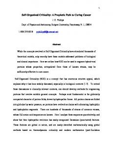
FIG. 3. The contour plot of r ( p,q) of the Domany-Kinzel model, Eq. ~1!, for a lattice of L52000 sites and t54000. The resolution is 1283128 bits. White corresponds to r 50 and the contour lines are drawn at 0.1 intervals.
obtained in just one simulation by iterating two-dimensional fragments. The plot of the asymptotic density r (p,q) is shown in Fig. 3. It compares well with those obtained with other methods @11,16,17#. From the convergent behavior of the contour lines, the position ( p51/2,q51) of the discontinuous transition for the density is clearly indicated. Near the corner ( p51,q50) the surface becomes irregular: this is due to the prevalence of the XOR in Eq. ~1!. One can also investigate the chaotic phase of the DK model by iterating two fragment configurations with the same random numbers. The Hamming distance between two replicas with a given value of p and q is the (p,q) component of the density of the XOR between the two asymptotic fragment configurations. A plot of the resulting Hamming distance is shown in Fig. 4. Here one can notice a trace of the density phase boundary @near (p50.8,q50)#, due to the critical slowing down. For the directed site percolation problem we found p c 50.7055(4), b 50.210 65(5), n 51.7195(5) for a system of size 106 , in the interval 0.7, p,0.71 for different values of a 51024,2048,4096,8192. The agreement with previous measurements @8# is satisfactory. Moreover, we want to stress that these values were obtained with data coming from simulations of less than 20 min of CPU time on a 150 MHz PC running LINUX @22#. As a second application, we consider now the kinetic version of an equilibrium system, the two-dimensional Ising model with heat bath dynamics @23,24#. In Appendix A we show how to express the evolution equation of this model as a totalistic PCA, and how to translate its evolution in fragment language. In Fig. 5 we show the plot of the magnetization m(p) with respect to p5exp(22J) for an Ising model with reduced interaction constant J. The transition is well characterized by plotting the second moment ~standard deviation! of the magnetization as a function of p. We found
3974
F. BAGNOLI, P. PALMERINI, AND R. RECHTMAN
55
FIG. 6. The diagram showing the mapping from criticality to self-organized criticality.
FIG. 4. The contour plot of the asymptotic value of the distance between two replicas of the system evolving under the same realization of the noise. The parameters are those of the previous figure.
p c 50.17260.002 and b 50.1160.002, in good agreement with the exact values p c 5( A221) 2 and b 51/8. IV. CRITICALITY AND SELF-ORGANIZED CRITICALITY
We have shown how the DK model and the Ising model, which are PCA with critical behavior, may be mapped into
fragment models with no control parameter, that is, models that show self-organized criticality ~SOC!. It is evident that the fragment method may be applied to any critical PCA. This result is summarized in the diagram of Fig. 6. The state x ti (p) may be obtained by evolving the PCA with a given p ~labeled by f p in the diagram! or by building the fragments X 0i and evolving them with the fragment method (F in the diagram! that does not depend on p. Finally, by probing X ti with a p layer, that is, by checking if X ti extends down to p, we recover x ti . Although it is easier to think of onedimensional fragments, this result is valid for any number of control parameters. It is interesting to describe a ‘‘traditional’’ SOC model with the fragment language, trying to obtain the p layer description that would make the SOC model correspond to a usual critical model.
FIG. 5. The magnetization m and the susceptibility Var(m) ~fluctuation of the magnetization! for a two-dimensional Ising model of size L51003100, averaging over 10 samples every 1000 time steps after a transient of 10 000 time steps. The resolution is 32 bits.
55
ALGORITHMIC MAPPING FROM CRITICALITY TO . . .
Let us discuss the one-dimensional Bak-Snappen model @10# with nearest-neighbor interactions. In this model one starts from an array of real numbers a i , i51, . . . ,L, uniformly distributed in the unit interval. One looks for the minimum of a i and replaces it and its nearest neighbors with newly generated random numbers, again uniformly distributed in the unit interval. The system auto-organizes so that the distribution of a i follows a power law ~with exponent 1!, with a nontrivial avalanche distribution. We define now a parallel version of the previous model ~which is not very efficient from a computational point of view!. For the sake of simplicity, we divide the discussion in two parts: the research of the minimum and the actual evolution. Let us visualize the a i as the lower extremum of segments ~fragments! X i , and cut the configuration with a line at height p. The minimum is localized at site k, for which there is only one intersection. It can be expressed using a Boolean variable d ti,k ~a Kronecker d )
d ti,k 5~ x ti ~ p ! „ jÞi ` x tj ~ p ! …, p
~11!
assuming that the minimum is unique in the continuous p limit. The fragments X i at and nearest to the minimum are replaced by segments of random length @ R(r)#, X t11 5X ti % ~ D ti21,k ~D ti,k ~D ti11,k ! „R ~ r ti ! % X ti …, i
~12!
where the fragment D ti,k is completely filled if d ti,k 51 and completely empty if D ti,k 50. The evolution can be expressed on a p layer as x t11 5x ti % ~ d ti21,k ~ d ti,k ~ d ti11,k !~@ r ti ,p # % x ti ! . i
~13!
Similar but more complex expressions can be found for the invasion percolation process. One can see that in these ‘‘traditional’’ SOC models there are long range space interactions, and also interactions among p layers @see Eq. ~11!#. We think that the second ingredient is the most important: if one knows how some quantity like the density varies with p, it is not difficult to imagine a mechanism that automatically reaches the critical point. It is still to be proved that this is the actual mechanism of SOC. On the other hand, Eq. ~8! shows that there exists space and p-local mechanisms that can be classified as SOC. V. CONCLUSIONS
The fragment method can be considered both as a recipe for numerical studies of phase diagrams and as a mapping from criticality to self-organized criticality. For what concerns the first topic, the possibility of having a sketch of the phase diagram without huge computation resources is useful in determining the position of the critical line. Numerical applications of the fragment method will be presented in future work. From the theoretical point of view, we think that the formalism presented in this work allows a clear characterization of the basic properties of self-organized models, suggesting analogies between usual critical phenomena and self-organized ones.
3975
ACKNOWLEDGMENTS
We wish to acknowledge fruitful discussions with P. Grassberger and R. Bulajich. Partial economic support from CNR ~Italy!, CONACYT ~Mexico!, Project DGAPA-UNAM IN103595, Centro Internacional de Ciencias A.C., the Programma Vigoni of the Conferenza Permanente dei Rettori delle Universita` Italiane, and the workshop Chaos and Complexity at ISI-Villa Gualino under the CE Contract No. ERBCHBGCT930295 is also acknowledged. APPENDIX: THE ISING MODEL
Let us start by considering the one-dimensional Ising model. Its reduced Hamiltonian can be written as J H~ x! 52 2
L21
(
i50
s i s i11 ,
~A1!
where s i 52x i 21 and x i 50,1. We choose the heat bath dynamics @23,24#, for which the probability t (x˜y… of going from a configuration x to a configuration y that can differ from x in a certain number $ i k % of sites is
t (x˜y)5
exp„2H~ y! … , ( 8 exp„2H~ y8 ! …
~A2!
where the sum in the denominator extends over all combinations of the differing sites y i k . This transition probability does not depend on x and satisfies the detailed balance principle. The configuration y is not limited to differ from x only at one site: the evolution can be applied in parallel changing all even ~or odd! sites. Since the transition probabilities do not depend on the previous value of the cell, the space-time lattice decouples into two noninteracting sublattices: one with even sites at even times and odd site at odd times, and the complementary one. By considering only one sublattice, the neighborhood of the one-dimensional Ising model is the same as that of the Domany-Kinzel model. The kinetic Ising model is just a totalistic cellular automaton ~without adsorbing states!. The local transition probabilities t (x i21 ,x i11 →y i ) can be computed from Eq. ~A2! considering a difference in just one site. They are
t ~ 0,0→1 ! 5 p/ ~ 11 p ! , t ~ 1,0→1 ! 51/2,
t ~ 0,1→1 ! 51/2,
t ~ 1,1→1 ! 51/~ 11 p ! ,
with p5exp(22J). It is convenient to introduce here the totalistic functions c k that take the value 1 if the sum of the variables in the neighborhood is k and zero otherwise. An efficient way of building these functions is described in @19#. For the Domany-Kinzel neighborhood they are c 0 5x 2 ~x 1 ,
c 1 5x 2 % x 1 ,
c 2 5x 2 x 1 .
The evolution equation for the Ising cellular automaton is x 8 5 @ r,p/ ~ 11 p !# c 0 ~ @ r,1/2# c 1 ~ @ r,1/~ 11p !# c 2 . ~A3!
3976
55
F. BAGNOLI, P. PALMERINI, AND R. RECHTMAN
Before using the fragment method one has to invert the @ r, f (p) # „@ r. f (p) # … expressions and substitute them with ¯ „f 21 (r)…#; p-independent expressions like R„f 21 (r)…@R R (0) according with r. We @ r,1/2# trasform to R(0) or ¯ leave them in the equations with the assumption that a true value means R(0) and a false value means ¯ R (0). We finally find that ¯ X 8 5R
S D
S D
r 12r C 0 1 @ r,1/2# C 1 1R C2 , 12r r
~A4!
X 8 5R
J 2
r r 1 C ~R C ~ r, C 2 12r 0 12r 1 2
¯ 12r C ~R ¯ ~R 3 r
12r C 4, r
~A6!
where p5exp(22J). The C k functions can be computed efficiently using the homogeneous polynomials D j @19#, C 0 5C 1 ~C 2 ~C 3 ~C 4 ,
where now the C k are fragments. For the 2D square Ising model with heat bath dynamics, the Hamiltonian is H~ x! 52
SA D S D F G S D SA D
C 2 5D 2 % D 3 ,C 3 5D 3 ,
C 1 5D 1 % D 3 , C 4 5D 4 ,
L21
(
i, j50
s i, j s i11,j 1 s i, j s i, j11
~A5!
where D 1 5X 11 % X 12 % X 21 % X 22 ,
with s i, j 52x i, j 21. The lattice decouples again in two noninteracting sublattices. Repeating the procedure as above, one has again a totalistic cellular automaton. Using the totalistic functions C k of four nearest neighbors, we find that
D 2 5X 11 X 12 % ~ X 11 % X 12 !~ X 21 % X 22 ! % X 21 x 22 ,
@1# D. Sornette, A. Johansen, and I. Dornic, J. Phys. I ~France! 5, 325 ~1995!. @2# S. Maslov and Y.-C. Zhang, Phys. Rev. Lett. 75, 1550 ~1995!. @3# M. Paczuski, S. Maslov, and P. Bak, Phys. Rev. E 53, 414 ~1996!. @4# D. Sornette and I. Dornic, Phys. Rev. E 54, 3334 ~1996!. @5# P. Grassberger and Y.-C. Zhang, Physica A 224, 169 ~1996!. @6# P. Bak, C. Tang, and K. Wiesenfeld, Phys. Rev. Lett. 59, 381 ~1987!. One can find an extended listing of articles on several aspects of SOC in the previously cited papers. @7# The original presentation occurred at ISI-Villa Gualino during the workshop Chaos and Complexity ~Torino, Italy, 1994!. See also Refs. @20,1,5#. @8# J.W. Essam, A.J. Guttmann, and K. de’Bell, J. Phys. A 16, 3815 ~1983!. @9# D. Wilkinson and J.F. Willemsen, J. Phys. A 16, 3365 ~1983!. @10# P. Bak and K. Sneppen, Phys. Rev. Lett. 71, 4083 ~1993!. @11# E. Domany and W. Kinzel, Phys. Rev. Lett. 53, 311 ~1984!; W. Kinzel, Z. Phys. B 58, 229 ~1985!. @12# A. Georges and P. Le Doussal, J. Stat. Phys. 54, 1011 ~1989!.
@13# H. J. Herrmann, J. Stat. Phys. 2, 145 ~1991!; D. Stauffer, J. Phys. A 24, L691 ~1991!. @14# K. Iverson, A Programming Language ~Wiley, New York, 1962!. @15# R. L. Graham, D. E. Knuth, and O. Patashnik, Concrete Mathematics ~Addison Wesley, New York, 1989!. @16# F. Bagnoli, J. Stat. Phys. 85, 151 ~1996!. @17# F. Bagnoli, R. Bulaijch, R. Livi, and A. Maritan, J. Phys. A 25, L1071 ~1992!. @18# I. Wegener, The Complexity of Boolean Functions ~Wiley, New York, 1987!. @19# F. Bagnoli, Int. J. Mod. Phys. C 3, 307 ~1992!. @20# S. Roux, A. Hansen, and E. Guyon, J. Phys. ~Paris! 48, 2125 ~1987!. @21# T. Halpin-Healy and Y.-C. Zhang, Phys. Rep. 254, 215 ~1995!. @22# http://www.cs.helsinki.fi/linux @23# A.M. Maritz, H.L. Herrmann, and L. de Arcangelis, J. Stat. Phys. 59, 1043 ~1990!. @24# F. Wang and M. Suzuki, Physica A 220, 534 ~1995!.
D 3 5D 2 D 1 ,
D 4 5X 11 X 12 X 21 X 22 .