Algorithmic Resource Verification - LARA and EPFL

Algorithmic Resource Verification

THÈSE N◦ 7885 (2017)

présentée le 9th November 2017 à la Faculté Informatique et Communications Laboratoire d’analyse et des raisonnement automatises programme doctoral en Informatique et communications ÉCOLE POLYTECHNIQUE FÉDÉRALE DE LAUSANNE pour l’obtention du grade de Docteur ès Sciences

PAR

Ravichandhran KANDHADAI MADHAVAN

acceptée sur proposition du jury: Prof. M. Odersky, président du jury Prof. V. Kuncak, directeur de thèse Prof. R. Majumdar, rapporteur Dr G. Ramalingam, rapporteur Prof. J. Larus, rapporteur

Suisse 2017

This thesis is dedicated to my maternal grandmother. Observing her I learnt what it means to work hard and be devoted.

Acknowledgements As I reflect upon my journey through my PhD I feel a sense of elation but at the same time an overwhelming sense of gratitude to many people who made me realize this dream. I take this opportunity to thank them all. First and foremost, I thank my advisor Professor Viktor Kuncak for the very many ways in which he has helped me during the course of my PhD. It is impossible for me to imagine a person who would have more faith and confidence in me than my advisor. His presence felt like having a companion with immense knowledge and experience who is working side-by-side with me towards my PhD. Besides his help with the technical aspects of the research, he was a great source of moral support. He shared my elation and pride when I was going through a high phase, my disappointment and dejection during paper rejections, and my effort, nervousness and excitement while working on numerous submission deadlines. I also thank him for all the big responsibilities that he had trusted me with: mentoring interns, managing several aspects of teaching like setting up questions, leading teaching assistants and giving substitute lectures. These were great experiences that I, retrospectively, think I am very fortunate to have had. I am very grateful to him that he had overlooked many of my blunders and mistakes in discharging my responsibilities and have always been very kind and supportive. Since it is impossible to elucidate all ways in which he has helped me, I would conclude by saying that I would always be proud to be called his advisee and I hope that I can live up to the trust and confidence he has in me in the future as well. I thank Dr. G. Ramalingam for being a constant source of inspiration and guidance all through my research career. He has helped me in my career in numerous ways: first as a great teacher, later as a great mentor and always as a great, supportive friend. I developed and honed much of my research skills by observing him. What I find amazing and contagious is his rational and deep reasoning not just about research problems but also about issues in life. I hope to have absorbed a bit of that skill having been in close acquaintance with him for these many years. I thank him for motivating me to pursue a PhD, to join EPFL and to work with my advisor. This thesis would not have been possible without his advise and motivation. I am very happy and proud that this dissertation is reviewed by him. I thank Professor Martin Odersky for being an excellent teacher and a source of inspiration. I greatly enjoyed the conversations we had and enjoyed working with him as a teaching assistant. I am very grateful to him for being very supportive about my research, and for presiding over the defense jury. I thank other members of the defense committee: Professor Jim Larus and Professor Rupak Majumdar for reviewing my dissertation and providing me very valuable i

Acknowledgements comments and feedback on the research, despite their very busy schedules. I greatly enjoyed discussing my research with them. I thank Pratik Fegade and Sumith Kulal who in the course of their internships helped with improving the system and the approach described in this dissertation. Particularly, I thank Pratik Fegade for contributions to the development of the techniques detailed in section 3.8 of this dissertation, and Sumith Kulal for helping carry out many experiments detailed in section 5. I thank my current and past lab mates Mikaël Mayer, Jad Hamza, Manos Koukoutos, Nicolas Voirol, Etienne Kneuss, Tihomir Gvero, Regis Blanc, Eva Darulova, Manohar Jonalagedda, Ivan Kuraj, Hossein Hojjat, Phillipe Suter, Andrew Reynolds, Mukund Raghothaman, Georg Schimd, Marco Antognini, Romain Edelmann, and also many other friends and colleagues. I enjoyed the numerous discussions I had with them in the lab, over meals, during outing and in every other place we were caught up in. In their company I felt like a truly important person. In particular, I thank Mikaël Mayer for being an amazing friend and collaborator all through my PhD life – with him I could freely share my successes as well as my frustrations. I thank Fabien Salvi for providing great computing infrastructure and for accommodating each and every request of mine no matter how urgent and time constrained they were. I thank Sylvie Jankow for her kindness and help with administrative tasks. Furthermore, I thank Professor K.V. Raghavan for being an excellent advisor of my master’s thesis and for being a constant source of encouragement. I thank him for persuading me to continue with a research career and eventually pursue PhD. I am also thankful to him and Professor Deepak D’Souza for introducing me to the area of program analysis. I fell in love with this amazing field at that very instant, and it feels like the rest of my research path was a foregone conclusion. I thank Dr. Sriram Rajamani for being a great source of inspiration and support in my research career. Last but not least, I thank my amazing family for their never ending love, support and sacrifices. I thank my parents for, well, everything I am today. I thank my sister, my grandmother and my brother-in-law for their limitless love and support. I thank my nieces Abi and Apoorva for showing me that life outside research can also be awesome. It is a wonder to me that they were born, grew and went to school while I was still pursuing my PhD. And, of course, I thank my wife Nikhila for her love and encouragement and, more importantly, for tolerating all my quirks. I thank numerous other friends, colleagues and relatives who I, unfortunately, could not mention but have made my PhD years the best phase in my life so far. Lausanne, August 2017

ii

Ravichandhran Kandhadai Madhavan

Preface Is the program I have written efficient? This is a question we face from the very moment we discover what programming is all about. The improvements in absolute performance of hardware systems have made this question more important than ever, because analytical behavior becomes more pronounced with large sizes of the data that today’s applications manipulate. Despite the importance of this question, there are surprisingly few techniques and tools that can help the developer answer such questions. Program verification is an active area of research, yet most approaches for software focus on safety verification of the values that the program computes. For performance, one often relies on testing, which is not only very incomplete, but provides little help in capturing the reasons for the behavior of the program. This thesis presents a system that can automatically verify efficiency of programs. The verified bounds are guaranteed to hold for all program inputs. The prototypical examples of resources are time (for example, the number of operations performed), or notions related to memory usage (for example, the number of allocation steps performed). These bounds are properties of the algorithms, not of the underlying hardware implementation. The presented system is remarkable in that it suffices for the developers to provide only sketches of the bounds that are expected to hold (corresponding to expected asymptotic complexity). The system can infer the concrete coefficients automatically and confirm the resource bounds. The paradigm supported by the approach in this thesis is purely functional, making it feasible to consider verification of very sophisticated data structures. Indeed, a “by product” of this thesis is that the author verified a version of rather non-trivial Conc Trees data structure that was introduced by Dr. Aleksandar Prokopec, and that play an important role in parallel collections framework of Scala. The thesis deals with subtleties of verifying performance of programs in the presence of higher-order functions. What is more, the thesis supports efficient functional programming in practice through treatment of the construct inspired by imperative behavior: memoization (caching). Memoization, and it special case, lazy evaluation, are known to improve efficiency of functional programs both in practice and in asymptotic terms, so they make functional programming languages more practical. Yet, reasoning about the performance in the presence of these constructs introduces substantial aspects of state into the model. The thesis shows how to make specification and verification feasible even under this challenging scenario.

iii

Preface Verification of program correctness has been a long road, and we are starting to see practical solutions that are cost-effective, especially for functional programs. With each step along this road, the gap in reasoning ability between developers and tools is narrowing. The work in this thesis makes a big step along an under-explored dimension of program meaning—reasoning about performance bounds. Given the extent to which program development is driven by performance considerations, closing this gap is likely to have not only great benefits for verifying programs, but will also open up new applications that leverage reliable performance information to improve and adapt software systems. The tools are waking up to the notion of verified performance as program metric, and this will make them even more profoundly important for software development. Lausanne, Summer 2017

iv

Viktor Kunˇcak

Abstract Static estimation of resource utilization of programs is a challenging and important problem with numerous applications. In this thesis, I present new algorithms that enable users to specify and verify their desired bounds on resource usage of functional programs. The resources considered are algorithmic resources such as the number of steps needed to evaluate a program (steps) and the number of objects allocated in the memory (alloc). These resources are agnostic to the runtimes and platforms on which the programs are executed yet provide a concrete estimate of the resource usage of an implementation. Our system is designed to handle sophisticated functional programs that use recursive functions, datatypes, closures, memoization and lazy evaluation. In our approach, users can specify in the contracts of functions an upper bound they expect to hold on the resource usages of the functions. The upper bounds can be expressed as templates with numerical holes. For example, a bound steps ≤ ?*size(inp) + ? denotes that the number of evaluation steps is linear in the size of the input inp. The templates can be seamlessly combined with correctness invariants or preconditions necessary for establishing the bounds. Furthermore, the resource templates and invariants are allowed to use recursive and first-class functions as well as other features supported by the language. Our approach for verifying such resource templates operates in two phases. It first reduces the problem of resource inference to invariant inference by synthesizing an instrumented first-order program that accurately models the resource usage of the program components, the higher-order control flow and the effects of memoization, using algebraic datatypes, sets and mutual recursion. The approach solves the synthesized first-order program by producing verification conditions of the form ∃∀ using a modular assume/guarantee reasoning. The ∃∀ formulas are solved using a novel counterexample-driven algorithm capable of discovering strongest resource bounds belonging to the given template. I present the results of using our system to verify upper bounds on the usage of algorithmic resources that correspond to sequential and parallel execution times, as well as heap and stack memory usage. The system was evaluated on several benchmarks that include advanced functional data structures and algorithms such as balanced trees, meldable heaps, Okasaki’s lazy data structures, streams, sorting algorithms, dynamic programming algorithms, and also compiler phases like optimizers and parsers. The evaluations show that the system is able to infer hard, nonlinear resource bounds that are beyond the capability of the existing approaches. Furthermore, the evaluations presented in this dissertation show that, when averaged over many benchmarks, the resource consumption measured at runtime is 80% of v

Abstract the value inferred by the system statically when estimating the number of evaluation steps and is 88% when estimating the number of heap allocations. Key words: verification, static analysis, complexity, resource usage, decision procedures

vi

Résumé L’analyse statique de la consommation en resources des programmes est un problème important avec de nombreuses applications possibles. Dans cette thèse, je présente de nouveaux algorithmes pour vérifier la consommation en ressources des programmes fonctionnels, algorithmes qui permettent aux utilisateurs de spécifier à leur guise des limites en resources, et de les vérifier. Les ressources considérées sont des ressources dites algorithmiques, comme par exemple le nombre d’étapes nécessaires pour évaluer un programme (steps) ou le nombre total d’objets qu’il crée en mémoire (alloc). Ces resources sont indépendantes de la plate-forme, bien qu’elles fournissent une mesure concrète de la consommation des implémentations d’algorithmes. Notre système peut analyser des programmes fonctionnels sophistiqués qui comportent des fonctions récursives, des données typées, des fonctions ayant capturé des variables (fermetures), des mises en cache (mémoïsations) ou des évaluations paresseuses. Grâce à notre approche, les utilisateurs peuvent, dans les contrats de fonctions, spécifier une limite supérieure à l’utilisation de ressources sous la forme de modèles à trous numériques, par exemple steps ≤ ?*size(l) + ?. Les limites en ressources peuvent être combinées avec des invariants ou des spécifications nécessaires à l’établissement de ces limites. Les limites en ressources et les invariants peuvent également utiliser des fonctions récursives et les fonctions elles-mêmes comme des valeurs, ainsi que d’autres fonctionnalités prises en charge par le langage que nous avons développé. L’approche visant à vérifier les modèles à trous comporte deux phases. La première phase réduit d’abord le problème de l’inférence des ressources en inférence d’invariant, en convertissant le programme en un programme instrumenté et du premier niveau (sans les fonctions comme valeurs). Ce programme modélise avec précision l’utilisation des ressources, le flux de contrôle de plus haut niveau et les effets de la mémoïsation, en utilisant des types de données algébriques, des ensembles et de la récursion mutuelle. La deuxième phase vérifie ce programme en produisant des conditions de vérification de la forme ∃∀ et en utilisant un raisonnement modulaire. Les formules ∃∀ sont résolues à l’aide d’un nouvel algorithme. Cet algorithme tire profit de contre-exemples pour découvrir les limites en ressources les plus précises pour le modèle donné. Je présente les résultats de l’utilisation de notre système, lorsque celui-ci vérifie le plus précisément possible les limites en les ressources algorithmiques qui correspondent aux temps d’exécution séquentiels et parallèles, ainsi qu’à l’utilisation de la mémoire du tas et de la pile. Nos tests, huit mille lignes de code en Scala, contiennent des arbres équilibrés comme les arbres bicolores, des tas fusionnables, l’analyse statique de la propagation de constantes, des algorithmes de tri paresseux comme le tri fusion paresseux, des structures de données vii

Résumé paresseuses comme les queues de temps constant d’Okasaki, des listes paresseuses cycliques, des parseurs et des algorithmes de programmation dynamique comme le problème du sac à dos. Les évaluations montrent que notre système est capable d’inférer de difficiles limites en ressources non linéaires, surpassant ainsi les approches existantes. Moyennés sur l’ensemble des tests, les résultats indiquent que, lors de l’exécution, la consommation en ressources est de 80 % de la valeur inférée par notre système lors de l’estimation de steps, et de 88 % lors de l’estimation de alloc. Mots clefs : vérification, analyse statique, complexité, utilisation des ressources, procédures de décision

viii

Contents Acknowledgements

i

Preface

iii

Abstract

v

List of figures 1 Introduction 1.1 Overview of the Specification Approach 1.1.1 Prime Stream Example . . . . . . 1.2 Summary of Contributions . . . . . . . 1.3 Outline of the Thesis . . . . . . . . . . .

xiii

. . . .

1 6 7 11 12

. . . . . . . . . . . . . . .

13 14 16 18 18 19 20 22 23 24 24 25 27 27 28 30

3 Solving Resource Templates with Recursion and Datatypes 3.1 Resource Instrumentation . . . . . . . . . . . . . . . . . . . . . . . . . . . . . . . . 3.1.1 Instrumentation for Depth . . . . . . . . . . . . . . . . . . . . . . . . . . . 3.2 Modular, Assume-Guarantee Reasoning . . . . . . . . . . . . . . . . . . . . . . .

31 32 34 37

. . . .

. . . .

. . . .

. . . .

2 Semantics of Programs, Resources and Contracts 2.1 Syntax of the Core Language . . . . . . . . . . 2.2 Notation and Terminology . . . . . . . . . . . . 2.3 Resource-Annotated Operational Semantics . 2.3.1 Semantic Domains . . . . . . . . . . . . 2.3.2 Resource Parametrization . . . . . . . . 2.3.3 Structural Equivalence and Simulation 2.3.4 Semantic Rules . . . . . . . . . . . . . . 2.4 Reachability Relation . . . . . . . . . . . . . . . 2.5 Contract and Resource Verification Problem . 2.5.1 Valid Environments . . . . . . . . . . . 2.5.2 Properties of Undefined Evaluations . . 2.5.3 Problem Definition . . . . . . . . . . . . 2.6 Proof Strategies . . . . . . . . . . . . . . . . . . 2.7 Properties of the Semantics . . . . . . . . . . . 2.7.1 Encapsulated Calls . . . . . . . . . . . .

. . . .

. . . . . . . . . . . . . . .

. . . .

. . . . . . . . . . . . . . .

. . . .

. . . . . . . . . . . . . . .

. . . .

. . . . . . . . . . . . . . .

. . . .

. . . . . . . . . . . . . . .

. . . .

. . . . . . . . . . . . . . .

. . . .

. . . . . . . . . . . . . . .

. . . .

. . . . . . . . . . . . . . .

. . . .

. . . . . . . . . . . . . . .

. . . .

. . . . . . . . . . . . . . .

. . . .

. . . . . . . . . . . . . . .

. . . .

. . . . . . . . . . . . . . .

. . . .

. . . . . . . . . . . . . . .

. . . .

. . . . . . . . . . . . . . .

. . . .

. . . . . . . . . . . . . . .

. . . .

. . . . . . . . . . . . . . .

. . . .

. . . . . . . . . . . . . . .

. . . .

. . . . . . . . . . . . . . .

. . . .

. . . . . . . . . . . . . . .

ix

Contents 3.2.1 Function-Level Modular Reasoning . . . . . . . . . . . . . . . . . . . . . .

37

3.2.2 Function-level Modular Reasoning with Templates . . . . . . . . . . . . .

42

3.3 Template Solving Algorithm . . . . . . . . . . . . . . . . . . . . . . . . . . . . . . .

42

3.3.1 Verification Condition Generation . . . . . . . . . . . . . . . . . . . . . . .

44

3.3.2 Successive Function Approximation by Unfolding . . . . . . . . . . . . .

47

3.3.3 Logic Notations and Terminology . . . . . . . . . . . . . . . . . . . . . . .

48

3.3.4 The solveUNSAT procedure . . . . . . . . . . . . . . . . . . . . . . . . . . .

49

3.4 Completeness of Template Solving Algorithm . . . . . . . . . . . . . . . . . . . .

55

3.4.1 Completeness of solveUNSAT Procedure . . . . . . . . . . . . . . . . . . .

55

3.5 Solving Nonlinear Formulas with Holes . . . . . . . . . . . . . . . . . . . . . . . .

62

3.6 Finding Strongest Bounds . . . . . . . . . . . . . . . . . . . . . . . . . . . . . . . .

63

3.7 Analysis Strategies and Optimizations . . . . . . . . . . . . . . . . . . . . . . . . .

64

3.8 Divide-and-Conquer Reasoning for Steps Bounds . . . . . . . . . . . . . . . . . .

65

3.9 Amortized Analysis . . . . . . . . . . . . . . . . . . . . . . . . . . . . . . . . . . . .

68

4 Supporting Higher-Order Functions and Memoization

71

4.1 Semantics with Memoization and Specification Constructs . . . . . . . . . . . .

72

4.1.1 Semantic Rules . . . . . . . . . . . . . . . . . . . . . . . . . . . . . . . . . .

74

4.2 Referential Transparency and Cache Monotonicity . . . . . . . . . . . . . . . . .

77

4.3 Proof of Referential Transparency . . . . . . . . . . . . . . . . . . . . . . . . . . .

78

4.4 Generating Model Programs . . . . . . . . . . . . . . . . . . . . . . . . . . . . . . .

81

4.4.1 Model Transformation . . . . . . . . . . . . . . . . . . . . . . . . . . . . . .

82

4.5 Soundness and Completeness of the Model Programs . . . . . . . . . . . . . . .

89

4.5.1 Correctness of Model Transformation . . . . . . . . . . . . . . . . . . . . .

92

4.5.2 Completeness of Model Transformation . . . . . . . . . . . . . . . . . . .

96

4.6 Model Verification and Inference . . . . . . . . . . . . . . . . . . . . . . . . . . . .

97

4.6.1 Creation-Dispatch Reasoning . . . . . . . . . . . . . . . . . . . . . . . . . .

99

4.7 Correctness of Creation-Dispatch Reasoning . . . . . . . . . . . . . . . . . . . . . 100 4.7.1 Partial Correctness of Creation-Dispatch Obligations . . . . . . . . . . . . 101 4.8 Encoding Runtime Invariants and Optimizations . . . . . . . . . . . . . . . . . . 107 5 Empirical Evaluation and Studies

111

5.1 First-Order Functional Programs and Data Structures . . . . . . . . . . . . . . . 112 5.1.1 Benchmark Descriptions . . . . . . . . . . . . . . . . . . . . . . . . . . . . 112 5.1.2 Analysis Results . . . . . . . . . . . . . . . . . . . . . . . . . . . . . . . . . . 115 5.1.3 Comparison with CEGIS and CEGAR . . . . . . . . . . . . . . . . . . . . . 118 5.2 Higher-Order and Lazy Data Structures . . . . . . . . . . . . . . . . . . . . . . . . 120 5.2.1 Measuring Accuracy of the Inferred Bounds . . . . . . . . . . . . . . . . . 121 5.2.2 Scheduling-based Lazy Data Structures . . . . . . . . . . . . . . . . . . . . 123 5.2.3 Other Lazy Benchmarks . . . . . . . . . . . . . . . . . . . . . . . . . . . . . 129 5.3 Memoized Algortihms . . . . . . . . . . . . . . . . . . . . . . . . . . . . . . . . . . 130 x

Contents

6 Related Work 135 6.1 Resource Analyses . . . . . . . . . . . . . . . . . . . . . . . . . . . . . . . . . . . . 135 6.2 Higher-Order Program Verification . . . . . . . . . . . . . . . . . . . . . . . . . . . 137 6.3 Software Verification . . . . . . . . . . . . . . . . . . . . . . . . . . . . . . . . . . . 138 7 Conclusion and Future Work

141

Bibliography

154

Curriculum Vitae

155

xi

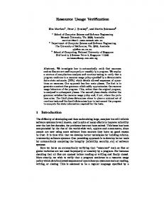
List of Figures 1.1 Relationship between number of steps and wall-clock execution time for a lazy selection sort implementation . . . . . . . . . . . . . . . . . . . . . . . . . . . . .

2

1.2 Illustration of verifying resource bounds using contracts . . . . . . . . . . . . . .

6

1.3 Prime numbers until n using an infinite stream. . . . . . . . . . . . . . . . . . . .

8

1.4 Specifying properties dependent on memoization state. . . . . . . . . . . . . . .

9

2.1 Syntax of types, expressions, functions, and programs . . . . . . . . . . . . . . .

15

2.2 Resource-annotated operational semantics of the core language . . . . . . . . .

17

2.3 Definition of the reachability relation . . . . . . . . . . . . . . . . . . . . . . . . .

24

3.1 Resource instrumentation for first-order programs. . . . . . . . . . . . . . . . . .

33

3.2 Illustration of instrumentation. . . . . . . . . . . . . . . . . . . . . . . . . . . . . .

33

3.3 Example illustrating the depth of an expression. . . . . . . . . . . . . . . . . . . .

34

3.4 Illustration of depth instrumentation. . . . . . . . . . . . . . . . . . . . . . . . . .

35

3.5 Instrumentation for the depth resource. . . . . . . . . . . . . . . . . . . . . . . .

36

3.6 Definition of the path condition for an expression belonging to a program P . .

39

3.7 Counter-example guided inference for numerical holes. . . . . . . . . . . . . . .

43

3.8 The solveUNSAT procedure . . . . . . . . . . . . . . . . . . . . . . . . . . . . . . .

50

4.1 Operational semantics of higher-order specifications and memoization. . . . .

73

4.2 Syntax and semantics of the set operations used by the model programs . . . .

82

4.3 A constant-time, lazy take operation . . . . . . . . . . . . . . . . . . . . . . . . . .

83

4.4 Illustration of the translation on lazy take example . . . . . . . . . . . . . . . . .

84

4.5 Representation of closure and cache keys . . . . . . . . . . . . . . . . . . . . . . .

84

4.6 Translation of types in a program P with a set of type declarations Tdef P . . . .

85

4.7 Resource and cache-state instrumentation of source expressions . . . . . . . . .

87

5.1 Benchmarks implemented as first-order functional Scala programs . . . . . . . 113 5.2 Results of running O RB on the first-order benchmarks . . . . . . . . . . . . . . . 115 5.3 Results of inferring bounds on depths of benchmarks . . . . . . . . . . . . . . . 117 5.4 Results of inferring bounds on the number of heap-allocated objects . . . . . . 117 5.5 Results of inferring bounds on the call-stack usage . . . . . . . . . . . . . . . . . 118 5.6 Higher-order, lazy benchmarks comprising 4.5K lines of Scala code . . . . . . . 120 5.7 Steps and Alloc bounds inferred by O RB for higher-order, lazy benchmarks . . . 120 xiii

List of Figures 5.8 Comparison of the resource usage bounds inferred statically against runtime resource usage . . . . . . . . . . . . . . . . . . . . . . . . . . . . . . . . . . . . . . . 5.9 Rotate function of the Real-time queue data structure . . . . . . . . . . . . . . . 5.10 Definition of Okasaki’s Real-time queue data structure . . . . . . . . . . . . . . . 5.11 Queue operations of Okasaki’s Real-time queue data structure . . . . . . . . . . 5.12 Invariants of conqueue data structure [Prokopec and Odersky, 2015] . . . . . . . 5.13 Comparison of the inferred bound (shown as grids) and the dynamic resource usage (shown as dots) for lazy merge sort . . . . . . . . . . . . . . . . . . . . . . . 5.14 Memoized algorithms verified by O RB . . . . . . . . . . . . . . . . . . . . . . . . 5.15 Accuracy of bounds inferred for memozied programs . . . . . . . . . . . . . . . . 5.16 Comparison of the inferred bound (shown as grids) and the dynamic resource usage (shown as dots) for Levenshtein distance algorithm . . . . . . . . . . . . . 5.17 Comparison of the inferred bound (shown as grids) and the dynamic resource usage (shown as dots) for ks . . . . . . . . . . . . . . . . . . . . . . . . . . . . . . .

xiv

121 124 125 126 128 130 131 131 132 132

1 Introduction

How fast can a computer program solve this problem? Answering this question is at the very heart of computer science. It wouldn’t be an exaggeration to say that the word fast in the above question primarily distinguishes computer science from conventional mathematics. Developing computer programs that solves a problem faster or with reduced resource usage is a subject of enormous practical value which has obsessed practitioners and theoreticians alike. This quest for better performance has led to remarkable algorithms and theoretical results, which are routinely implemented and deployed at large scales and thus profoundly influencing our modern civilization by driving scientific discoveries, commerce and social interaction. However, a question that developers are often faced with is whether an implementation of an algorithm conforms to the performance expected out of it. The techniques presented in this dissertation are aimed at addressing this challenge. Unfortunately, statically determining the resource usage of a program has proven to be very challenging. This is not only because the space of possible inputs of realistic programs is huge (if not infinite), but also because of the sophistication in the modern runtimes, like virtualization, on which the programs are executed. On the one hand this complexity poses serious impediment to developing automated tools that can help with reasoning about performance, on the other it has increased the need for developing such tools since programmers are also faced with similar (if not more) difficulties in analyzing the resource usage of programs. These challenges have resulted in wide ranging techniques for static estimation of resource usage of programs that model the resource usage at various levels of abstraction.

Algorithmic Resources Approaches such as those described by Wilhelm et al. [2008] and Carbonneaux et al. [2014] aim at estimating resource usage of programs in terms of concrete physical quantities (e.g. seconds, bytes etc.) under controlled environments, like embedded systems, for restricted class of programs where the number of loop iterations is a constant or is independent of the inputs. On the other extreme there are the static analysis tools that derive asymptotic upper bounds on the resource usage of general-purpose programs [Albert et al., 2012, Gulwani et al., 2009, Nipkow, 2015]. Using concrete physical quantities to measure 1

time (ms)/steps (in million)

Chapter 1. Introduction

1.6 1.4 1.2 1.0 0.8 0.6 0.4 0.2 0.0

kmin-steps kmin-time min-steps min-time

1

2

3

4 5 6 7 8 Size of list (in thousand)

9

10

Figure 1.1 – Relationship between number of steps and wall-clock execution time for a lazy selection sort implementation

resource usage has the disadvantage that they are specific to a runtime and hardware, and applicable to only restricted programs and runtimes. However, the alternative of using asymptotic complexities results in overly general estimates for reasoning about implementations, especially for applications like compiler optimizations or for comparing multiple implementations. For instance, a program executing ten operations on each input and another executing a million operations on every input have the same asymptotic complexity of O(1). For these reasons, recent techniques such as Resource Aware ML [Hoffmann et al., 2012, 2017] have resorted to more algorithmic measures of resource usage, such as the number of steps in the evaluation of an expression (commonly referred to as steps) or the number of memory allocations (alloc). These resources have the advantage that they are fairly independent of the runtime, but at the same time provide more concrete information about the implementations. This dissertation, which is a culmination of the prior research works: [Madhavan and Kuncak, 2014, Madhavan et al., 2017], further advances the static estimation of such algorithmic measures of resource usage to functional programs with recursive functions, recursive datatypes, first-class functions, lazy evaluation and memoization. Although the objective of our approach is not to compute bounds on physical time, our initial experiments do indicate a strong correlation between the number of steps performed at runtime and the actual wall-clock execution time for our benchmarks. Figure 1.1 shows a plot of the wall-clock execution time and the number of steps executed by a function that computes the k t h minimum of an unsorted list using a lazy selection sort implementation. The figure shows a strong correlation between one step performed at runtime and one nanosecond. (The bounds inferred by our tool in this case almost accurately matched the runtime steps usage for this benchmark as discussed in section 5.) Furthermore, for a lazy, bottom-up merge sort implementation [Apfelmus, 2009] one step of evaluation at runtime corresponded to 2.35 nanoseconds (ns) on average with an absolute deviation of 0.01 ns, and for a real-time queue 2

data structure implementation [Okasaki, 1998] it corresponded to 12.25 ns with an absolute deviation of 0.03 ns. These results further add to the importance of establishing resource bounds even if they are with respect to the algorithmic resource metrics.

Contracts for Resources Most existing approaches for analyzing resource usage of programs aim for complete automation but trade off expressive power and the ability to interact with users. Many of these techniques offer little provision for users to specify the bounds they are interested in, or to provide invariants needed to prove bounds of complex computation. For instance, establishing precise resource usage of operations on balanced trees requires the height or weight invariants that ensure balance. As a result, most existing approaches are limited in the programs and resources that they can verify. This is somewhat surprising since resource usage is as hard and as important as proving correctness properties, and the latter is being accomplished with increasing frequency on large-scale, real-world applications such as operating systems and compilers, by using user specifications [Harrison, 2009, Hawblitzel, 2009, Kaufmann et al., 2000, Klein et al., 2009, Leroy, 2009]. This dissertation demonstrates that user-provided contracts are an effective means to make resource verification feasible on complex resources and programs that are well outside the reach of automated techniques. Moreover, it also demonstrates that the advances in SMT-driven verification technology, traditionally restricted to correctness verification, can be fully leveraged to verify resource usage of complex programs.

Specifying Resource Bounds Specifying resources using contracts comes with a set of challenges. Firstly, the resources consumed by the programs are not program entities that programmers can refer to. Secondly, the bounds on resources generally involve constants that depend on the implementations, and hence are difficult to estimate by the users. Furthermore, the bounds, and invariants needed to establish the bound, often contain invocations of user-defined recursive functions specific to the program being verified, such as size or height functions on a tree structure. Our system provides language-level support for a predefined set of algorithmic resources. These resources are exposed to the users through special keywords like steps or alloc. Furthermore, it allows users to specify a desired bound on the predefined resources as templates with numerical holes e.g. as steps ≤ ?*size(l) + ? in the contracts of functions along with other invariants necessary for proving the bounds. The templates and invariants are allowed to contain user-defined recursive functions. The goal of the system is to automatically infer values for the holes that will make the bound hold for all executions of the function. (Section 2 formally describes the syntax and semantics of the input language.)

Verifying Resource Specifications In order to verify such resource templates along with correctness specifications, I developed an algorithm for inferring an assignment for the holes 3

Chapter 1. Introduction that will yield a valid resource bound. Moreover, under certain restrictions (such as absence of nonlinearity) the algorithm infers the strongest possible values for the holes and infers the strongest bound feasible for a given template. Specifically, the following are the three main contributions of the inference algorithm. (a) It provides a decision procedure for a fragment of ∃∀ formulas with nonlinearity, uninterpreted functions and algebraic datatypes. (b) It scales to complex formulas whose solutions involved large, unpredicatable constants. (c) It handles highly disjunctive programs with multiple paths and recursive functions. The system was used to verify the worst-case resource usage of purely functional implementations of many complex algorithms including balanced trees and meldable heap data structures. For instance, it was able to establish that the number of steps involved in inserting into a red-black tree implementation provided to the system is bounded by 132blog(size(t) + 1))c + 66. The inference algorithm and the initial results appeared in the publication [Madhavan and Kuncak, 2014], and is detailed in Section 3.

Memoization and Lazy Evaluation Another challenging feature supported by our system are first-class functions that rely on (built-in) memoization and lazy evaluation. (Memoization refers to caching of outputs of a function for each distinct input encountered during an execution, and lazy evaluation means the usual combination of call-by-name and memoization supported by languages like Haskell and Scala.) These features are quite important. From a theoretical perspective, it was shown by Bird et al. [1997] that these features make the language strictly more efficient, in asymptotic terms, than eager evaluation. From a practical perspective, they improve the running time (as well as other resource usage) of functional programs sometimes by orders of magnitude. For instance, the entire class of dynamic programming algorithms is built around the notion of memoizing recursive functions. These features have been exploited to design some of most practically efficient, functional data structures known [Okasaki, 1998], and often find built-in support in language runtimes or libraries in various forms e.g. Scala’s lazy vals and stream library, C#’s LINQ library. However, in many cases, it has been notoriously difficult to make precise theoretical analysis of the running time of programs that uses lazy evaluation or memoization. In fact, precise running time bounds remain open in some cases (e.g. lazy pairing heaps described in page 79 of Okasaki [1998]). Some examples illustrative of this complexity are the Conqueue data structure [Prokopec and Odersky, 2015] used to implement Scala’s data parallel operations, and Okasaki’s persistent queues [Okasaki, 1998] that run in worst-case constant time. The challenge that arises with these features is that reasoning about resources like running time and memory usage becomes state-dependent and more complex than correctness. Nonetheless, they preserve the functional model (referential transparency) for the purpose of reasoning about the result of the computation making them more attractive and amenable to functional verification in comparison to imperative programming models. 4

Resource Verification with Memoization In this dissertation, I also show that the userdriven, contract-based approach can be effective in verifying complex resource bounds in this challenging domain: higher-order functional programs that rely on memoization and lazy evaluation. From a technical perspective, verifying resource usage with these features present unique challenges that are outside the purview of existing verifiers. For instance, consider a function take that returns the first n elements of a stream. If accessing the tail of the stream takes O(n) time then accessing n elements would take O(n 2 ) time. However, invoking the function take twice or more on the same list would make every call except the first run in O(n) time due to the memoization of the tail of the stream. (Figure 1.3 presents a concrete example.) Verifying such programs require invariants that depend on the state of the memoization table. Also in some cases, it is necessary to reason about aliasing of references to higher-order functions. This dissertation presents new specification constructs that allow users to specify such properties succinctly. It presents a multi-staged approach for verifying the specifications that gradually encodes the input program and specifications into ∃∀ formulas (VCs) that use only theories efficiently decidable by state-of-the-art SMT solvers. The resulting formulas i.e, VCs are solved using the inference algorithm discussed in the previous paragraph. The encoding was carefully designed so that it does not introduce any abstraction by itself. This meant that users can help the system with more specifications until the desired bounds are established, which adheres with the philosophy of verification. The main technical contributions of this approach are: (a) development of novel specification constructs that allow users to express properties on the state of the memoization table in the contracts and also specify the behavior of first-class functions passed as parameters, (b) design of a new modular, assume-guarantee reasoning for verifying state-dependent contracts in the presence of higher-order functions. This approach and related results appeared in a prior publication: [Madhavan et al., 2017], and is detailed Section 4.

Evaluation and Results The approach presented in this dissertation is implemented within the open-source L EON verification and synthesis framework [Blanc et al., 2013]. The implementation is free and open source and available at https://github.com/epfl-lara/leon. The implementation was used to infer precise resource usage of complex functional data structures – balanced trees, heaps and lazy queues, as well as program transformations, static analyses, parsers and dynamic programming algorithms. Some of these benchmarks have never been formally verified before even with interactive theorem provers. Furthermore, through rigorous empirical evaluation, the precision of the constants inferred by our tool was compared to those obtained by running the benchmarks on concrete inputs (for the resources steps and alloc). Our results confirmed that the bounds inferred by the tool were sound over-approximations of the runtime resource usage, and showed that the worst-case resource usage was, on average, at least 80% of the value inferred by the tool when estimating the number of evaluation steps, and is 88% for the number of heap-allocated objects. For 5

Chapter 1. Introduction

1 2 3 4 5 6

import leon.instrumentation._ import leon.invariant._ object ListOperations { sealed abstract class List case class Cons(head: BigInt, tail: List) extends List case class Nil() extends List

7

def size(l: List): BigInt = l match { case Nil() ⇒ 0 case Cons(_, t) ⇒ 1 + size(t) }

8 9 10 11 12

def append(l1: List, l2: List): List = (l1 match { case Nil() ⇒ l2 case Cons(x, xs) ⇒ Cons(x, append(xs, l2))

13 14 15 16

}) ensuring (res ⇒ size(res) == size(l1) + size(l2) && steps ≤ ? ∗size(l1) + ?)

17 18 19 20 21 22 23 24 25

}

def reverse(l: List): List = { l match { case Nil() ⇒ l case Cons(hd, tl) ⇒ append(reverse(tl), Cons(hd, Nil())) } } ensuring (res ⇒ size(res) == size(l) && steps ≤ ? ∗(size(l)∗size(l)) + ?)

Figure 1.2 – Illustration of verifying resource bounds using contracts

instance, our system was able to infer that the number of steps spent in accessing the k t h element of an unsorted list l using a lazy, bottom-up merge sort algorithm [Apfelmus, 2009] is bounded by 36(k · blog (l .si ze)c) + 53l .si ze + 22. The number of steps used by this program at runtime was compared against the bound inferred by our tool by varying the size of the list l from 10 to 10K and k from 1 to 100. The results showed that the inferred values were 90% accurate for this example. To the best of my knowledge, our tool is the first available system that can establish such complex resource bounds with this degree of automation.

1.1 Overview of the Specification Approach In this section, I provide a brief overview of how to express programs and specifications in our system using pedagogical examples, and summarize the verification approach. This section is aimed at highlighting the challenges involved in verifying the resource usage of programs that are considered in this dissertation. It also provides an overview of a few specification constructs supported by our system, which will be formally introduced in the later chapters. Consider the Scala program shown in Figure 1.2 that defines a list as a recursive datatype and defines three operations on it. This example is aimed at highlighting the deep inter6

1.1. Overview of the Specification Approach relationships between verifying correctness properties and resource bounds. The function size computes the size of the list, the function append concatenates a list l2 to a list l1, and the function reverse reverses the list by invoking append and itself recursively. Consider the function reverse. The resource template shown in the postcondition of reverse specifies that the number of steps performed by this function is quadratic in the size of the list. The goal is to infer a bound that satisfies this template. Intuitively, the reason for this quadratic complexity is because the call to append that happens at every recursive step of reverse takes time linear in the size of the argument passed to it: tl (which equals l.tail). To establish this we need two facts: (a) the function append takes time that is linear in the size of its first formal parameter. (b) The size of the list returned by reverse is equal to the size of the input list, since append is invoked on the list returned by the recursive call to reverse. Therefore, we have the predicate: size(res)== size(l) in the postcondition of reverse. However, in order to establish this, we also need to know the size of the list returned by append in terms of the sizes of its inputs. This necessitates a postcondition for append which asserts that the size of the list returned by append is equal to sum of the sizes of the input lists. Thus, to verify the steps bound, one requires all the invariants specified in the program. This example also illustrates the need for an expressive contract language, since even for this small program we need all the invariants shown in the figure to verify its resource bounds. A major feature offered by our system is that it allows seamless combination of such userdefined invariants with resource templates. The invariants are utilized during the verification of resource bounds to verify the bound and also infer precise values for the constants. The system inferred the bound 11size(l)2 + 2 for the function reverse.

1.1.1 Prime Stream Example In this section, I illustrate specification and verification of programs with higher-order features and lazy evaluation using the pedagogical example shown in Figure 1.3 that creates an infinite stream of prime numbers. The example also illustrates some of the novel specification constructs that are supported by our system for proving precise bounds of such programs. The class SCons shown in Figure 1.3 defines a stream that stores a pair of unbounded integer (BigInt) and boolean, and has a generator for the tail: tfun which is a function from Unit to SCons. The lazy field tail of SCons evaluates tfun() when accessed the first time and caches the result for reuse. The program defines a stream primes that lazily computes for all natural numbers starting from 1 its primality Notice that the second argument of the SCons assigned to primes is a lambda term (anonymous function) that calls nextElem(2), which when invoked creates a new stream that applies nextElem to the next natural number and so on. The function isPrimeNum(n) tests the primality of n by checking if any number greater than 1 and smaller than n divides n using an inner function rec. The number of steps it takes is linear in n. The function primesUntil returns all prime numbers until the parameter n using a helper

7

Chapter 1. Introduction

1 2 3 4

private case class SCons(x: (BigInt,Bool), tfun:() ⇒ SCons) { lazy val tail = tfun() } private val primes = SCons((1, true), () ⇒ nextElem(2))

5 6 7 8 9 10 11

def nextElem(i: BigInt): SCons = { require(i ≥ 2) val x = (i, isPrimeNum(i)) val y = i + 1 SCons(x, () ⇒ nextElem(y)) } ensuring(r ⇒ steps ≤ ? ∗ i + ?)

12 13 14 15 16 17 18 19 20 21 22

def isPrimeNum(n: BigInt): Bool = { def rec(i: BigInt): Bool = { require(i ≥ 1 && i < n) if (i == 1) true else (n % i != 0) && rec(i − 1) } ensuring (r ⇒ steps ≤ ? ∗ i + ?) rec(n − 1) } ensuring(r ⇒ steps ≤ ? ∗ n + ?)

23 24 25 26 27

def isPrimeStream(s: SCons, i: BigInt): Bool = { require(i ≥ 2) s.tfun ≈ (() ⇒ nextElem(i)) }

28 29 30 31 32 33 34 35 36 37 38

def takePrimes(i: BigInt, n: BigInt, s: SCons): List = { require(0 ≤ i && i ≤ n && isPrimeStream(s, i+2)) if(i < n) { val t = takePrimes(i+1, n, s.tail) if(s.x._2) Cons(s.x._1, t) else t } else Nil() } ensuring(r ⇒ steps ≤ ? ∗ (n(n−i)) + ?)

39 40 41 42 43

def primesUntil(n: BigInt): List = { require(n ≥ 2) takePrimes(0, n−2, primes) } ensuring(r ⇒ steps ≤ ? ∗ n2 + ?)

Figure 1.3 – Prime numbers until n using an infinite stream.

function takePrimes, which recursively calls itself as long as i < n on the tail of the input stream (line 32), incrementing the index i . Consider now the running time of this function. If takePrimes is given an arbitrary stream s, its running time cannot be bounded since accessing the field tail at line 32 could take any amount of time. Therefore, we need to know the resource 8

1.1. Overview of the Specification Approach

1 2 3 4

def concrUntil(s: SCons, i: BigInt): Bool = if(i > 0) cached(s.tail) && concrUntil(s.tail, i−1) else true

5 6

def primesUntil(n: BigInt): List = {

7 8

// see Figure 1.3 for the code of the body

9 10 11 12 13

} ensuring{r ⇒ concrUntil(primes, n−2) && (if(concrUntil(primes, n−2) in inSt) steps ≤ ? ∗ n + ? else steps ≤ ? ∗ n2 + ?) }

Figure 1.4 – Specifying properties dependent on memoization state. usage of the closures accessed by takePrimes, namely s.(tail)∗ .tfun. However, we expect that the stream s passed to takePrimes is a suffix of the primes stream, which means that tfun is a closure of nextElem. To allow expressing such properties our system reintroduces the notion of intensional or structural equivalence, denoted ≈, between closures [Appel, 1996].

Structural Equality as a means of Specification In our system, closures are allowed to be compared structurally. Two closures are structurally equal iff their abstract syntax trees are identical without unfolding named functions. This equivalence is formally defined in section 2.3. For example, the comparison at line 27 of Figure 1.3 returns true iff the tfun parameter of s is a closure that invokes nextElem on an argument that is equal to i. This equality is found to be an effective and low-overhead means of specification for the following reasons. (a) Many interesting data structures based on lazy evaluation use aliased references to closures (e.g. Okasaki’s scheduling-based data structures [Okasaki, 1998, Prokopec and Odersky, 2015] discussed in section 5.2). Expressing invariants of such data structures requires equating closures. While reference equality is too restrictive for convenient specification (and also breaks referential transparency), semantic or extensional equality between closures is undecidable, and hence introduces high specification/verification burden. Structural equality is well suited in this case. (b) Our approach is aimed at (but not restricted to) callee-closed programs where the targets of all indirect calls are available at analysis time. (Section 2.3 formally describes such programs.) In such cases, it is often convenient and desirable to state that a closure has the same behavior as a function in the program, as was required in Figure 1.3. (c) Structural equality also allows modeling reference equality of closures by augmenting closures with unique identifiers as they are created in the program. While structural equality is a well-studied notion [Appel, 1996], to my knowledge, no prior 9

Chapter 1. Introduction work uses it as a means of specification. Using structural equality, it can be specifed that the stream passed as input to takePrimes is an SCons whose tfun parameter invokes nextElem(i+2) (see function isPrimeStream and the precondition of takePrimes). This allows the system to bound the steps, which denotes the number of primitive evaluation steps, of the function takePrimes to O(n(n − i )) and that of primesUntil to O(n 2 ). For primesUntil, our tool inferred that steps ≤ 16n 2 + 28.

Properties Dependent on Memoization State. The quadratic bound of primesUntil is precise only when the function is called for the first time. If primesUntil(n) is called twice, the time taken by the second call would be linear in n, since every access to tail within takePrimes will take constant time as it has been cached during the previous call to takePrimes. The time behavior of the function depends on the state of the memoization table (or cache) making the reasoning about resources imperative. To specify such properties the system supports a built-in operation cached(f(x)) that can query the state of the cache. This predicate holds if the function f is a memoized function and is cached for the value x. Note that it does not invoke f(x). The function concrUntil(s, i) shown in Figure 1.4 uses this predicate to state a property that holds iff the first i calls to the tail field of the stream s have been cached. (Accessing the lazy field s.tail is similar to calling a memoized function tail(s).) This property holds for primes stream at the end of a call to primesUntil(n), and hence is stated in the postcondition of primesUntil(n) (line 10 of Figure 1.4). Moreover, if this property holds in the state of the cache at the beginning of the function, the number of steps executed by the function would be linear in n. This is expressed using a disjunctive resource bound (line 11). Observe that in the postcondition of the function, one need to refer to the state of the cache at the beginning of the function, as it changes during the execution of the function. For this purpose, our system supports a built-in construct “inSt" that can be used in the postcondition to refer to the state at the beginning of the function, and an “in" construct which can be used to evaluate an expression in the given state. These expressions are meant only for use in contracts. These constructs are required since the cache is implicit and cannot be directly accessed by the programmers to specify properties on it. On the upside, the knowledge that the state behaves like a cache is exploited by the system to reason functionally about the result of the functions, which results in fewer contracts and more efficient verification.

Verification Strategy. Our approach, through a series of transformations, reduces the problem of resource bound inference for programs like the one shown in Figure 1.3 to invariant inference for a strict, functional first-order program. It solves it by applying an inductive, assume-guarantee reasoning. The inductive reasoning exploits and uses the monotonic evolution of cache, and the properties that are monotonic with respect to the changes to the cache. 10

1.2. Summary of Contributions The inductive reasoning works on the assumption that the expressions in the input program terminate, which is verified independently using an existing termination checker. Our system uses the Leon termination checker for this purpose [Nicolas Voirol and Kuncak, 2017], but other termination algorithms for higher-order programs [Giesl et al., 2011, Jones and Bohr, 2004, Sereni, 2006] are also equally applicable. Note that memoization only affects resource usage and not termination, and lazy suspensions are in fact lambdas with unit parameters. This strategy of decoupling termination checks from resource verification enables checking termination using simpler reasoning, and then use proven well-founded relations during resource analysis. This allows us to use recursive functions for expressing resource bounds and invariants, and enables modular, assume-guarantee reasoning that relies on induction over recursive calls (previously used in correctness verification) to establish resource bounds. This aspect is discussed in more detail in section 3.2.

1.2 Summary of Contributions In summary, the following are the major contributions of this dissertation: I. I propose a specification approach for expressing resource bounds of programs and the necessary invariants in the presence of recursive functions, recursive datatypes, first-class functions, memoization and lazy evaluation. • The approach allows specifying bounds as templates with numerical holes in the postconditions of functions, which are automatically solved by the system (section 2). • The specifications can use structural-equality-based constructs for specifying properties of higher-order functions (section 2). • The specification can assert properties on the state of the memoization table (section 3). II. I present a system for verifying the contracts of programs expressed in our language by designing new algorithms and extending existing techniques from contract-based correctness verification. • I present a novel inference algorithm for solving ∃∀ formulas with recursive functions, inductive datatypes and nonlinearity such as multiplication of two unknown variables. I prove that the algorithm is sound, always terminates, and also is complete under certain restrictions (section 3.3). • I present an encoding of higher-order functions with memoization as first-order programs with recursive functions, dataypes and sets, and establish its soundness and completeness (section 4.4). • I present an assume-guarantee reasoning for higher-order functions with memoization, 11

Chapter 1. Introduction which exploits properties that monotonically evolve with respect to the changes in the cache. I establish the soundness of this reasoning (section 4.6). III. I present the results of using the system to establish precise resource bounds of 50 benchmarks, comprising 8K lines of functional Scala code, implementing complex data structures and algorithms that are outside the reach of existing approaches. The experimental evaluations show that while the inferred values always over-estimate the runtime values, the runtime values are 80% of the value inferred by the tool when averaged over all benchmarks (section 5).

1.3 Outline of the Thesis The rest of the dissertation is organized as follows:

• Chapter 2 describes the core syntax and semantics of the input language and specifications. It formalizes the semantics of the resources supported by our system. It defines the problem of resource and contract verification, and formally establishes several properties of the core language. • Chapter 3 describes the algorithm for inferring resource bounds for first-order programs without higher-order features and memoization. It details the resource instrumentation performed by our system, the modular assume-guarantee reasoning used by system, and the inference algorithm for inferring holes. • Chapter 4 describes the extensions to the algorithm for inferring resource bounds of programs with first-class functions and memoization. It formally describes the semantics of memoization and related specification constructs. It formally presents and proves the verification approach that can handle programs with these features. • Chapter 5 presents the results of evaluation of the system on the benchmarks using summary statistics and graphical plots. It also presents the fully verified implementation of the real-time queue data structure. • Chapter 6 discusses the works related to the topic of this dissertation.

12

2 Semantics of Programs, Resources and Contracts The purpose of abstraction is not to be vague, but to create a new semantic level in which one can be absolutely precise. — Edsger W. Dijkstra In this chapter, I formally present and discuss the core syntax and semantics of the programs accepted by our system and eventually define the problem of resource verification. As a first step, I introduce a core language that captures the relevant syntactic aspects of the input programs. Specifically, the core language supports recursive functions, recursive datatypes, contracts and resource templates. For the sake of succinctness and reducing notational overhead, for certain constructs of the core language I adopt the syntax of lambda calculus instead of following the syntax of Scala. For instance, anonymous functions are denoted as λ terms and variable declarations are replaced by “let" binders. Nonetheless, the constructs of the language have a straightforward translation to Scala. The syntax description of the language also includes higher-order constructs, lazy evaluation and memoization, and specification constructs meant for use with these features. However since these features are quite involved and are orthogonal to the definition of the problem, in this chapter I will focus mostly on first-order constructs and defer the discussion of the semantics of other constructs to later chapters. The semantics I present here is a big-step, operational semantics that has two unorthodox features. Firstly, the semantics not only characterizes the state changes induced by the language constructs but also characterizes their resource usage. To succinctly formalize usage of multiple resources supported by our system, the semantics is parameterized by “cost" functions. These cost functions capture resource-specific parameters and are independently (re)defined for each resource that is of interest. I also present the definition of these cost functions for the important resources supported by our system: steps, alloc, stack and depth. The second unorthodox feature of the semantics is that it assigns an operational meaning to contracts and specification constructs. Thus contracts in our system are expressions of the 13

Chapter 2. Semantics of Programs, Resources and Contracts language and, in principle, are executable on an appropriate runtime that can implement their semantics. This naturally allows contracts to use and manipulate the same entities used by the rest of the program. For instance, the variables, data structures and functions declared in the program are automatically available to the predicates in the contracts without restriction. In the final sections of this chapter, I define the problem of contract and resource verification for open programs (or libraries) and define notions like encapsulation using the operational semantics of the constructs of the language. These definitions are used to establish the soundness of our system in the later chapters (Chapters 3 and 4).

2.1 Syntax of the Core Language Figure 2.1 show the syntax of the core functional language describing the syntax of the input programs. Esrc shows the syntax of the expressions that can be used in the implementation. They consists of variables Vars, constants Cst, primitive operations on integers and booleans Prim, a structural equality operator eq, let expressions, match expressions, lambda terms, direct calls to named functions: f x, and indirect calls or lambda applications: x y. The rule Blockα is parameterized by the subscript α and defines the let, match and if-then-else combinators that operate over a base expression e α . The integers in our language are unbounded big integers. They correspond to the BigInts of Scala. Tdef shows the syntax of user-defined recursive datatypes and Fdef shows the syntax of function definitions. The functions are classified into source functions Fdefsrc , which are considered as implementations, and specification functions Fdefspec , which can be used only in the specifications (explained shortly). As a syntactic sugar, tuples are considered as a special datatype. Tuple constructions are denoted using (x 1 , · · · , x n ), and selecting the i t h element of a tuple is denoted using x.i . For ease of formalization, the language incorporates the following syntactic restrictions without reducing generality. Most expressions except lambda terms are expressed in A-normal form i.e, the arguments of the operations performed by the expressions are variables. The conditional expressions such as if-then-else and match constructs are an exception, since the expressions along the branches need to be executed only when the corresponding guards are true. All lambdas are of the form: λx. f (x, y) where f is a named function whose argument is a pair (a two element tuple) and y is a captured variable. Note that this lifting of bodies of lambda terms to named functions is a simple syntactic refactoring which does not limit the expressiveness of the language. Every expression belonging to our language has a static label belonging to Labels (not shown in Figure 2.1). For instance, the label of an expression e could a combination of the name of the source file that contains the expression e and the position of e in the source file. Let e` denotes an expression with its label. To reduce clutter, the labels are omitted if it is not relevant to the context. A program P is a set of functions definitions in which every function identifier is unique, every direct call invokes a function defined in the program, and the labels of all expressions are unique. 14

2.1. Syntax of the Core Language

x, y ∈ Vars

(Variables)

c ∈ Cst

(Variables & Constants)

f ∈ Fids

(Function Identifiers)

d ∈ Dids

(Datatype identifiers)

C i ∈ Cids, i ∈ N

(Constructor Identifiers)

a ∈ TVars

(Template Variables)

x¯ ∈ Vars∗

(Sequence of Variables)

τ¯ ∈ Vars

(Sequence of Types)

∗

Tdef

::=

¯ · · · ,C n τ) ¯ type d := (C 1 τ,

τ ∈ Type

::=

Unit | Int | Bool | τ ⇒ τ | d

Blockα

::=

let x := e α in e α | x match{(C x¯ ⇒ e α ; )+ } | if (x) eα else eα

pr ∈ Prim

::=

+ | − | ∗ | ··· | ∧ | ¬

e s ∈ Esrc

::=

x | c | pr x | x eq y | f x | C x¯ | e λ | x y | Block s

e λ ∈ Lam

::=

λx. f (x, y)

e p ∈ Espec

::=

e s | Block p | ( f p x) | res | resource ≤ ub | Emem | x fmatch {(e λ ⇒ e p ; )+ }

Emem

::=

cached( f x) | inSt | outSt | in(e p , x) | e p ?

resource

::=

steps | alloc | stack | depth

ub ∈ Bound

::=

ep | et

e t ∈ Etmp

::=

a · x + et | a

Fdefsrc

::=

(@memoize )? def fs x := {ep } es {ep }

Fdefspec

::=

def fp x := {ep } ep {ep }

Fdef

::=

Fdefsrc ∪ Fdefspec

Program

::=

2(Tdef ∪Fdef )

Figure 2.1 – Syntax of types, expressions, functions, and programs

The annotation @memoize serves to mark functions that have to be memoized. Such functions are evaluated exactly once for each distinct input passed to them at run time. Notice that only source functions are allowed to be memoized. The language as such uses call-by-value evaluation strategy. But this annotation allows the language to simulate call-by-need or lazy evaluation strategy. This feature is discussed in detail in section 4. Expressions that are bodies of functions can have contracts (also called specifications). Such expressions have the form {e1 } e {e2 } where e 1 and e 2 are the pre-and post-conditions of e respectively. These conditions can use constructs that are not available to the source expressions. In other words, their syntax given by Espec permits more constructs than Esrc . In particular, the postcondition of an expression e can refer to the result of e using the variable res, and can 15

Chapter 2. Semantics of Programs, Resources and Contracts refer to the resource usage of e using the keywords steps, alloc or depth. Users can specify upper bounds on resources as templates with holes as defined by et ∈ Etmp . The holes always appear as coefficients of variables defined or visible in the postconditions. The variables could be bound to more complex expressions through let binders. We enforce that the holes are distinct across function definitions. The specification constructs fmatch and those given by Emem are meant for specifying the behavior of first-class functions and the behavior of expressions under memoization, respectively. I will not focus on these constructs here and will explain them in detail in Chapter 4. Before I discuss the formal semantics of the language, I present a few basic notation and terminology used in the rest of the sections.

2.2 Notation and Terminology Partial Functions Given a domain A, a¯ ∈ A ∗ denotes a sequence of elements in A, and a i refers to the i t h element. Note that this is different from tuple selector x.i , which is an expression of the language. The notation A 7→ B denotes a partial function from A to B . Given ˆ x) ¯ denotes the function that applies h point-wise on each element of a partial function h, h( ¯ h[a 7→ b] denotes the function that maps a to b and every other value x in the domain of x. ¯ denotes h[a 1 7→ b 1 ] · · · [a n 7→ b n ]. The function h is omitted h to h(x). The notation h[a¯ 7→ b] in the above notation if it is an empty function. Let h 1 ] h 2 be defined as (h 1 ] h 2 )(x) = if (x ∈ dom(h2 )) h2 (x) else h1 (x). Let h1 v h2 iff the function h 2 includes all binding of h 1 i.e, ∀a ∈ dom(h 1 ).h 1 (a) = h 2 (a). A closed integer interval from a to b is denoted using [a, b].

Expression Operations Let labelsP denote the set of labels of all expressions in a program P . Let typeP (e) denote the type of an expression e in a program P . Given an expression e, let FV (e) denote the set of free variables of e. Expressions without free variables are referred to as closed expressions. Given a lambda term λx. f (x, y), y is called the captured variable of the lambda term. Note that FV (eλ ) is a singleton set containing the captured variable. target(eλ ) denotes the function called in the body of the lambda. (Recall that the body of every lambda term is call to a named function. ) The operation e[e 0 /x] denotes the syntactic replacement of the free occurrences of x in e by e 0 . This operation replaces expressions along with their static labels and also performs alpha-renaming of bound variables, if necessary, to avoid variable capturing. A substitution ς : Vars 7→ Expr is a partial function from variables to expressions. Let e ς denote e[ς(x 1 )/x 1 ] · · · [ς(x n )/x n ], where dom(ς) = {x 1 , · · · x n }. Given a substitution ι : TVars 7→ Z, let e ι represent the substitution of the holes by the values given by the assignment. Similarly, let P ι denote the program obtained by replacing the every hole a in the bodies of functions in P by ι(a). This notation is also extended to formulas later. Programs and expressions without holes as referred to as concrete programs and expressions. Let body P ( f ) and paramP ( f ) denote the body and parameter of a function f defined in a program P 16

2.2. Notation and Terminology

C ST

VAR

P RIM

c ∈ Cst

x ∈ Vars

pr ∈ Prim

Γ ` c ⇓ c, Γ

Γ : (H, σ) ` x ⇓ σ(x), Γ

Γ ` pr x ⇓ pr(σ(x)), Γ

ccst

cvar

E QUAL

L ET

v = σ(x) ≈ σ(y)

Γ ` e1 ⇓p v1 , (H 0 , σ0 )

H

Γ : (H, σ) ` x eq y ⇓ v, Γ

C ONS

clo = (λx. f (x, y), [y 7→ σ(y)])

a = fresh(H)

(H 0 , σ[x 7→ v1 ]) ` e2 ⇓q v2 , (H 00 , σ00 )

Γ : (H, σ) ` let x := e1 in e2

ceq

L AMBDA

cpr

(H, σ) ` cons x¯ ⇓ a, (H 0 , σ) ccons

Cλ

(H, σ[x¯i 7→ v¯ ]) ` ei ⇓q v, (H 0 , σ0 )

H(σ(x)) = C i v¯

Γ : (H, σ) ` x match {Ci x¯i ⇒ ei )}ni=1 IF

Γ ` ei ⇓q v, Γ0

Γ ` if (x) e1 else e2 ⇓ v, Γ0

⇓

cmatch(i) ⊕q

where i =

v, (H 0 , σ)

( 1 σ(x) = true

0 σ(x) = false

cif ⊕q

D IRECT C ALL

C ONCRETE C ALL

(H, σ[paramP (f ) 7→ u]) ` body P (f ) ⇓p v, (H 0 , σ0 )

f ∈ Fids

Γ : (H, σ) ` f u ⇓p v, (H 0 , σ) A PP

H(σ(x)) = (λz.e, σ0 )

Γ ` pre ⇓p true, Γ1

Γ ` (f σ(x)) ⇓p v, Γ0

Γ`f x

⇓

ccall ⊕p

v, Γ0

(H, (σ ] σ0 )[z 7→ σ(y)]) ` e ⇓p v, (H 0 , σ0 )

Γ : (H, σ) ` x y C ONTRACT

v2 , (H 00 , σ)

ˆ x))] ¯ H 0 = H[a 7→ (cons σ(

a = fresh(H)

Γ : (H, σ) ` λx.f (x, y) ⇓ a, (H[a 7→ clo], σ) M ATCH

⇓

clet ⊕p⊕q

Γ ` e ⇓q v, Γ2 : (H2 , σ2 )

⇓

capp ⊕p

v, (H 0 , σ)

(H2 , σ2 [R 7→ q, res 7→ v]) ` post ⇓r true, Γ3

Γ ` {pre} e {post} ⇓q v, Γ2 where R ∈ {steps, alloc, stack, depth}

cmatch(i) = i + 1 cvar = clet = 0 Cost function definition for steps: cop = 1 ⊕=+ ccons = cλ = 1 cop = 0 Cost function definition for alloc: ⊕=+

for every other operation op

for every other operation op

Figure 2.2 – Resource-annotated operational semantics of the core language 17

Chapter 2. Semantics of Programs, Resources and Contracts

2.3 Resource-Annotated Operational Semantics Figure 2.2 defines the operational semantics for the core language that also captures the resource consumption of expressions of the language. The semantics is defined only for concrete expressions without holes. (Expressions with holes are not executable.) The semantics is big-step which is well suited for formalizing a compositional approach such as ours. Unfortunately, big-step semantics is not convenient for reasoning about termination or reachability of states at a specific expression (or program point), both of which are necessary for our purposes. Therefore, I define a reachability relation on top of the big-step semantics, similar to the calls relation of Sereni, Jones and Bohr [Jones and Bohr, 2004, Sereni, 2006]. This reachability relation acts similar (but not identical) to a small-step semantics.

2.3.1 Semantic Domains The semantics rules presented in Figure 2.2 operate over the semantics domain described below. Let Adr denote the addresses of heap-allocated structures namely closures and datatypes. Let DVal denote the set of datatype instances, Clo the set of closures. Let H be a partial function from addresses to datatypes instances or lambdas and a store σ a partial function from variables to values. The state of an interpreter evaluating expressions of our language, referred to as the evaluation environment Γ, is a triple consisting a heap H, a store σ, and a program, which is a set of function definitions. Formally, u, v ∈ Val = Z ∪ Bool ∪ Adr DVal = Cids × Val∗ Clo = Lam × Store H ∈ Heap = Adr 7→ (DVal ∪ Clo) σ ∈ Store = V ar s 7→ Val Γ ∈ Env ⊆ Heap × Store × Program Every environment should also satisfy the following domain invariants, which are certain sanity conditions that are ensured by the operation semantics. Def 1 (Domain Invariants). A triple (H, σ, P ) is an environment iff the following properties hold. (a) (range(σ) ∩ Adr) ⊆ d om(H) (b) x ∈ dom(σ) implies that σ(x) inhabits typeP (x) (c) a ∈ dom(H) implies that H(a) inhabits typeP (a) (d) H is a acyclic heap (e) For all closures (λx. f (x, y), σ0 ) ∈ range(H), f is defined in P and y ∈ dom(σ0 ) In the above definition the type of an address is the same as the type of the constructor or lambda term that it refers to. The invariant (d) requiring the heap to be acyclic is defined more 18

2.3. Resource-Annotated Operational Semantics formally in section 2.7. Let fresh(H) be a function that picks an address that is not bound in the heap H. That is fresh(H) ∈ (Adr \ d om(H)). Such a function can be defined deterministically by fixing a well-ordering on the elements of Adr and requiring that fresh(H) always returns the smallest address not bound in the heap H. That is, fresh(H) = min(Adr \ dom(H)).

Judgements Let Γ ` e ⇓p v, Γ0 be a semantic judgement denoting that under an environment Γ ∈ Env, an expression e evaluates to a value v ∈ Val and results in a new environment Γ0 ∈ Env, while consuming p ∈ Z units of a resource. When necessary Γ is expanded as Γ : (H, σ, P ) to highlight the individual components of the environment. Any component of the judgement that is not relevant to the discussion is omitted when there is no ambiguity. In Figure 2.2, the program component is omitted from the environment as it does not change during the evaluation.

2.3.2 Resource Parametrization The operational semantics is parameterized in a way that it can be instantiated on multiple resources using the following two cost functions: (a) A cost function c op that returns the resource requirement of an operation op such as cons or app. The operation c op may possibly have parameters. In particular, c mat ch(i ) is used to denote the cost of a match operation when the i t h case is taken, which should include the cost of failing all the previous cases. (b) A resource combinator ⊕ : Z∗ → Z that computes the resource usage of an expression by combining the resource usages of the sub-expressions. Typically, ⊕ is either + or max. The Figure 2.2 shows the definition of the cost functions for resources: (a) the number of steps in the evaluation of an expression denoted steps, and (b) the number of heap-allocated objects created by an expression (viz. a closure or datatype) denoted alloc. For both resources, the resource combinator ⊕ is defined as addition (+). In the case of steps, c let and c var are zero as the operations are normally optimized away or subsumed by a machine instruction. The cost of every other operation is 1 except for c match(i) . The cost of the match operation (c match(i) ) is defined proportional to i as the cost of failing all the i − 1 match cases has to be included. Datatype constructions and primitive operations on integers (which are unbounded big integers in our language) are considered as unitary steps. In the case of alloc, c op is 1 for datatype and closure creations as they involve heap allocations. It is zero for every other operation. Another resource supported by our tool is the number of (call) stack locations required for holding the local variables and results of function calls during the evaluation of an expression, denoted stack. This resource can also be expressed using the cost functions. A somewhat simplified definition is shown below. 19

Chapter 2. Semantics of Programs, Resources and Contracts ⊕ = max Cost function definition for stack: ccall = capp = 1 + # of local variables of the callee cop = 0 for every other operation op

In the above definition, the number of local variables of the callee is given by the number of let-binders in the expression body( f ) for a direct call f x or an application applying a lambda λx. f (x, y). Note that when the above definition of ⊕ is plugged into the semantics, the stack usage of a let expression: let x := e 1 in e 2 would be computed as the maximum of the stack usages of e 1 and e 2 . This is the expected semantics as the stack space utilized by the calls made during e 1 could be reclaimed and reused during the evaluation of e 2 . The above definition is a much simplified version that hides many complexities. For instance, the number of arguments passed to call and applications are assumed to be one as, in our core language, every function take only one argument – two or more arguments have to be passed (by reference) via a tuple, which is allocated in the heap. Secondly, the actual parameter passing mechanism of a runtime may reserve more space in the call stack more than required for allocating local variables of a function. However, these constant factors (if they are precisely known) can be captured by the cost functions quite easily. In addition to the above resource, our system also supports a resource depth, which is a measure of algorithmic parallel execution time. However, defining the resource is slightly more involved. The discussion of this resource is deferred to section 3, where the instrumented procedure is described. Our tool also supports a resource rec that counts the number of recursions that appear in the evaluation and is useful for bounding the asymptotic complexity.

2.3.3 Structural Equivalence and Simulation As shown in Figure 2.1 our language supports an equality operator eq for comparing expressions of the language. The semantics shown in Figure 2.2 defines this operation using a structural equivalence relation ≈ defined on the values Val with respect to a H ∈ Heap (see H

rule E QUALS). This equivalence is explained and defined below. Two addresses are structurally equivalent iff they are bounded to structurally equivalent values in the heap. Two datatypes are structurally equivalent iff they use the same constructor and their fields are equivalent. Structural equivalence of closures is similar to syntactic equality of lambdas modulo alpha renaming (but extended to captured variables). Two closures are structurally equivalent iff their lambdas are of the form λx. f (x, y) and λw. f (w, z) and the captured variables y and z are bound to structurally equivalent values. Formally, ≈ is defined H

as the least fix point of the following equations. (The subscript ≈ is omitted below for clarity). H

20

2.3. Resource-Annotated Operational Semantics ∀a ∈ Z ∪ B ool . ∀{a, b} ⊆ Ad r. ∀ f ∈ Fids, {a, b} ⊆ Val. ¯ ⊆ Valn . ∀c ∈ Cids, {¯a, b} ∀{e1 , e2 } ⊆ Lam. ∀{σ1 , σ2 } ⊆ Store.

a≈a a ≈ b iff H(a) ≈ H(b) ( f a) ≈ ( f b) iff a ≈ b ¯ iff ∀i ∈ [1, n].ai ≈ bi (c a¯ ) ≈ (c b) (e 1 , σ1 ) ≈ (e 2 , σ2 ) iff target(e 1 ) = target(e 2 ) ∧σ1 (FV (e 1 )) ≈ σ2 (FV (e 2 ))

For datatypes, this equivalence is similar to value equality supported by languages like Scala and ML, and for closures this equivalence is similar to the traditional notion of intensional equality. Although not supported by modern languages since Lisp 1.5, intensional equality proved to be quite a powerful and handy tool in specifying resource usage behavior of firstclass functions. One of the contributions made by this dissertation is that constructs based on intensional equality of closures offer a referentially transparent yet decidable notion of equality between closures (as opposed to reference or extensional equality) and hence provide great value from the perspective of specifications, especially for proving implementationdependent properties like resource consumption. These aspects are considered in more detail in Chapter 4.

Structural Simulation Relation While the above described structural equivalence serves to compared two values under the same H, it is often required in the formalism to compare values under different heaps that arise during independent evaluations. For instance, to show a program transformation is equivalent to the original program, one needs to show that they agree on all values, which could be addresses defined under multiple heaps. For these purposes, I define a structural simulation relation ≈ with respect to two heaps as shown H1 ,H2

below. This relation is primarily used in the proofs of soundness and completeness of the algorithms. (The subscripts H1 , H2 are omitted in the following definitions for clarity.)

∀a ∈ Z ∪ B ool . ∀{a, b} ⊆ Ad r. ∀ f ∈ Fids, {a, b} ⊆ Val. ¯ ⊆ Valn . ∀c ∈ Cids, {¯a, b} ∀{e1 , e2 } ⊆ Lam.∀{σ1 , σ2 } ⊆ Store.

a≈a a ≈ b iff H1 (a) ≈ H2 (b) ( f a) ≈ ( f b) iff a ≈ b ¯ iff ∀i ∈ [1, n].ai ≈ bi (c a¯ ) ≈ (c b) (e 1 , σ1 ) ≈ (e 2 , σ2 ) iff target(e 1 ) = target(e 2 ) ∧σ1 (FV (e 1 )) ≈ σ2 (FV (e 2 ))

Notice that the only change compared to the definition of structural equivalence (≈) is the rule H

for addresses which now uses different heaps. The following are some properties of structural simulation. (The proof of the following properties are omitted as they are straightforward to derive from the definitions.) 21

Chapter 2. Semantics of Programs, Resources and Contracts (i)

If H1 v H2 , ≈ is equivalent to ≈

(ii)

x ≈ y implies y ≈ x

(iii)

x ≈ y and y ≈ z implies x ≈ y

H1 ,H2

H1 ,H2 H1 ,H2

H2

(Symmetry)

H2 ,H1

H2 ,H3

H1 ,H3

(Transitivity)

Note that the first property above implies relexivity. The definition of structural equivalence between values can be lifted to stores and environments in a natural way as shown below. ∀{σ1 , σ2 } ⊆ Store. σ1 ≈ σ2 iff dom(σ1 ) = dom(σ2 ) ∧ ∀x ∈ dom(σ1 ).σ1 (x) ≈ σ2 (x) H1 ,H2

H1 ,H2

∀Γ1 : (H1 , σ1 , P ), Γ2 : (H2 , σ2 , P ). Γ1 ≈ Γ2 iff σ1 ≈ σ2 H1 ,H2

Structural equivalence as defined above is a congruence relation with respect to the operational semantics. That is, evaluation of an expression e under structurally equivalent environments produces structurally equivalent environment and result values, and also has identical resource usage. Lemma 1. For all {Γ1 , Γ2 } ⊆ Env such that Γ1 ≈ Γ2 , for all expression e, Γ1 ` e ⇓p u, Γ1 0 =⇒ ∃v, q, Γ2 0 . Γ2 ` e ⇓q v, Γ2 0 ∧ Γ1 0 ≈ Γ2 0 ∧ u 0≈ 0 v ∧ p = q H1 ,H2

Proof. The claim directly follows by structural induction over the operation semantic rules shown in Fig. 2.2. This structural induction strategy is discussed in detail in section 2.6 later in this chapter.

2.3.4 Semantic Rules Consider now the semantics rules shown in Figure 2.2. Most rules are straightforward now that the cost functions and structural equivalence relations have been introduced. Below I describe some of the complex rules. The rule L AMBDA creates a closure for a lambda term t , which is a pair consisting of t , and a (singleton) assignment for the variable captured from the enclosing context, which is given by FV (t ). The rule C ONCRETE C ALL defines the semantics of a call whose arguments have been evaluated to concrete values (in Val). It models the call-by-value parameter passing mechanism: it binds the parameters to argument values, and evaluates the body (an expression with contracts) under the new binding. A call evaluates to a value only if the contracts of the callee are satisfied as given by the rule C ONTRACT (discussed shortly). This rule is used by the rule D IRECT C ALL which evaluates direct call expressions of the language. The handling of direct calls is separated from that of concrete calls whose arguments are values to make the semantics amenable to extensions for incorporating memoization (discussed in chapter 4). Concrete calls serve as the keys of the memoization table, which can be evaluated independently. 22

2.4. Reachability Relation The rule A PP handles applications of the form: x y. It first evaluates x to a closure (λz.e, σ0 ), and then evaluates e under the environment Γ : (H, (σ ] σ0 )[z 7→ σ(y)]), where the store (σ ] σ0 ) includes the assignment for the captured variables. Note that the assignment in σ0 takes precedence over σ for the captured variables, implying that the values of captured variables are frozen at the time of creation of the closure. The rule C ONTRACT defines the semantics of an expression e˜ of the form {pre} e {post} that has contracts. Though contracts are expressions of the language, they are considered to be different from implementation. They are treated as specifications that describe the expected behavior of the implementation rather than being a part of the implementation. They are expected to be statically proven and not checked at runtime (at least under normal scenarios). The expression e˜ evaluates to a value v only if pre holds in the input environment and post holds in the environment resulting after evaluating e. Observe that the value, heap effects, and resource usage of e˜ are equal to that of e. In other words, the resource usage and heap effects of evaluating the contracts are ignored. Also note that the resource variables (like steps) are bound to the resource consumption of e before evaluating the postcondition.

2.4 Reachability Relation One of the disadvantages of the big-step semantics is that when an evaluation of an expression under an environment is undefined, it could means two things: (a) either its evaluation diverges i.e, it does not terminate, or (b) its evaluation is stuck e.g. due a runtime exception or contract failure. In order to distinguish between these two situations, I define a relation called reachability relation inspired by the calls relation of Sereni [2006] and Jones and Bohr [2004] defined for a similar purpose. Intuitively, 〈Γ, e〉 〈Γ0 , e 0 〉 iff the big-step reduction of e under Γ requires reduction of e 0 under Γ0 . It is formally defined as follows. For every semantic rule shown in Figure 2.2 with n antecedents: A 1 · · · A m B 1 · · · B n , where A 1 · · · A n are not big-step reductions, and each B i , i ∈ [1, n], is a big-step reduction of the form: Γi ` ei ⇓pi vi , Γi 0 , the reachability relation has n rules for each 1 ≤ i ≤ n of the form: A1 · · · Am B 1 · · · B i −1 . Figure 2.3 presents the complete definition of this relation. 〈Γ, e〉 〈Γi , e i 〉 Note that the reach relation is quite different from a small-step operational semantics. Let ∗ represent the reflexive, transitive closure of . An environment Γ0 is said to reach e 0 during the evaluation of e under Γ iff 〈Γ, e〉 ∗ 〈Γ0 , e 0 〉.

Termination of Big-step Evaluation The evaluation of e under Γ is said to diverge or nonterminate iff there exists an infinite sequence 〈Γ, e〉 〈Γ1 , e 1 〉 · · · . An expression e (or a function f ) terminates iff there does not exist a Γ ∈ Env under which e (or body( f )) diverges [Sereni, 2006]. Since the evaluation of an expression under the big-step operational semantics proceeds as a derivation tree that is finitely branching, for a terminating evaluation, there is a 23

Chapter 2. Semantics of Programs, Resources and Contracts

L ET 2

L ET 1

〈Γ, let x := e 1 in e 2 〉 IF1

〈Γ, e 1 〉

〈Γ, let x := e 1 in e 2 〉 IF2

σ(x) = true

〈Γ, if (x) e 1 else e 2 〉

Γ ` e1 ⇓ v1 , (H 0 , σ0 ) 〈(H 0 , σ0 [x 7→ v 1 ]), e 2 〉

σ(x) = false

〈Γ, if (x) e 1 else e 2 〉

〈Γ, e 1 〉

〈Γ, e 2 〉

M ATCH

H(σ(x)) = C i v¯ 〈Γ : (H, σ), x match {C i x¯i ⇒ e i )}ni=1 〉

¯ ei 〉 〈(H, σ[x¯i 7→ v]), D IRECT C ALL

C ONCRETE C ALL

〈Γ : (H, σ), f u〉 A PP

B ODY

〈(H, (σ ] σ0 )[z 7→ σ(y)]), e〉 P OST

Γ ` pre ⇓ true

〈Γ, {pre} e {post}〉

〈Γ, e〉

〈Γ, f x〉

〈Γ, f σ(x)〉

P RE

H(σ(x)) = (λz.e, σ0 )

〈Γ : (H, σ), x y〉

f ∈ Fids

〈(H, σ[param( f ) 7→ u]), body( f )〉

Γ ` pre ⇓ true

〈Γ, {pre} e {post}〉

〈Γ, {pre} e {post}〉

〈Γ, pr e〉

Γ ` e ⇓q v, Γ2 : (H2 , σ2 ) 〈(H2 , σ2 [R 7→ q, res 7→ v]), post 〉

Figure 2.3 – Definition of the reachability relation

natural number n such that the length of every sequence of the form 〈Γ, e〉 〈Γ1 , e 1 〉 · · · is ¡ ¢ upper bounded by n. That is, ∃n ∈ N.¬ ∃k > n, e, Γ0 .〈Γ, e〉 k 〈Γ0 , e〉 iff e terminates under Γ.

2.5 Contract and Resource Verification Problem 2.5.1 Valid Environments While the semantics rules shown in Figure 2.2 may be applicable to arbitrary environments, in reality, the environments under which an expression is evaluated satisfies several invariants which are ensured either by the runtime (e.g. that every free variable in an expression is bound in the environment), or by the program under execution (e.g. that a value of a variable is always positive). As in prior works on data structure verification [Kapur et al., 2006], it is only reasonable to define the problem of contract/resource verification with respect to such valid environments under which an expression can be evaluated, instead of under arbitrary environments. For this purpose, I first define a notion of valid environments. Let P c = P 0 ||P denote a closed program obtained by composing a client P 0 with an open program P . Note that P c has to satisfy the requirements of the program namely that the labels 24

2.5. Contract and Resource Verification Problem of all expressions are unique, the function identifiers are unique etc. The evaluation of a closed program P c starts from a distinguished entry expression eentry such as a call to the main function under an initial environment ΓP c : (;, ;, ;, P c ). The valid environments of an expression e belonging to an open program P , denoted Enve,P , are the environments that reach e during some closed evaluation P 0 ||P . That is, © Enve,P = Γ | ∃P 0 .〈ΓP 0 ||P , eentry 〉

∗

〈Γ, e〉

ª

The valid environments reaching an expression may satisfy many properties beyond those ensured by the domain invariants. Though some of which could be program specific, some of them are ensured by the semantics itself. For instance, the following lemma states that in all valid environments reaching an expression e, every free variable of e would be bound to a value. Lemma 2. Let e be an expression in a program P and Γ : (H, σ, P ) ∈ Enve,P . FV (e) ⊆ d om(σ). The proof of the above lemma is easy to establish from the definition of Enve,P by inducting on the number of steps to reach 〈Γ, e〉 from a closed program 〈ΓP 0 ||P , eentry 〉.

2.5.2 Properties of Undefined Evaluations This section establishes an important property about the semantics presented in Figure 2.2. Under the assumption that all primitive operations are total, when an expression belonging to a type correct program is evaluated under a valid environment, there are only two reasons why its evaluation may be undefined as per the operational semantics: (a) the evaluation diverges, or (b) there is a contract violation during the evaluation. This property is very important since the definition of contract verification presented shortly relies on this property. Before formally establishing this property I state and prove a few important notions and lemmas. Def 2 (Contract Violation). Given an expression e˜ with contract: e˜ = {p} e {s}. The contract of e˜ ˜ 〈Γ0 , s〉 ∧ Γ0 ` s ⇓ false). is said to have been violated under Γ iff Γ ` p ⇓ false ∨ ∃Γ0 .(〈Γ, e〉 The following lemma states that whenever an evaluation of an expression is undefined under an environment then either the expression has a contract and is violated, or the evaluation of some (immediate) sub-expression of e is undefined. Lemma 3. Let e be an expression in a type-correct program P . Let Γ : (H, σ, P ) ∈ Env be such that FV (e) ⊆ dom(σ). If ¬∃v.Γ ` e ⇓ v then either e has a contract and is violated under Γ, or ∃Γ0 , e 0 .〈Γ, e〉 〈Γ0 , e 0 〉 and ¬∃v.Γ0 ` e0 ⇓ v. Proof. This property can be proved by exhaustively checking each of the semantic rules shown Fig. 2.2. Consider the rules C ST, VAR, E QUAL, L AMBDA, C ONS. Each of these rule do not have a big-step reduction in the antecedent. Every value required by the rule are either the output of 25

Chapter 2. Semantics of Programs, Resources and Contracts a total function like fresh which is always defined, or σ(x) or σ(H(x)), where x is a free variable in e 0 , and σ and H are the store and heap components of Γ0 . By definition, FV (e) ⊆ dom(σ), and Γ satisfies all the domain invariants. Thus, both σ(x) and σ(H(x)) are defined. Hence, the rules must be defined whenever the expression e matches the consequent. Now consider the rule A PP, C ONCRETE C ALL, D IRECT C ALL, M ATCH, I F, P RIM or L ET. In addition to requiring that σ(x) or σ(H(x)) are defined, these rule require more properties on shape (or type) of σ(x) in order to be defined for an expression matching the consequent. In the case of I NDIRECT C ALL, σ(H(x)) is required to be a closure. In the case of M ATCH, σ(H(x)) is required to be a datatype with the constructors that match the patterns in the M ATCH construct. In the case of P RIM, σ(x) should have the type of the argument of the primitive operation pr . (Recall that every primitive operation is total.) In the case of I F the condition should evaluate to a boolean. In the case of C ONCRETE C ALL the function identifier must have a definition in the program P . All of these are properties guaranteed by the type checker. Since Γ satisfies all the domain invariants, σ(x) should inhabit the typeP (x). Since it is given that the program P type checks, typeP (x) will satisfy the above requirements in each of the rules. Hence, every value required by these rules that are not big-step reductions will be defined. If every big-step reduction Γ0 ` e0 ⇓ v in the antecedent of these rules produce a value, then clearly ∃v.Γ ` e ⇓ v (see Fig. 2.2), because every other antecedent will be satisfied as explained above. Therefore, for evaluation of e to be undefined ∃Γ0 , e 0 .〈Γ, e〉 〈Γ0 , e 0 〉 and ¬∃v.Γ0 ` e0 ⇓ v. Now consider the rule C ONTRACT. Let e be an expression with contracts i.e, {p} e0 {s}. First, if the pre-or post-condition of e evaluates to false, the contract of e is violated and hence the claim holds. If e 0 evaluates to any value and p or s evaluate to true then e evaluates to a value. Therefore, for evaluation of e to be undefined e 0 or p or s does not evaluate to a value. Hence the claim.

Now it is easy to show that if an evaluation of an expression is undefined in a valid environment then either it has a contract violation or its evaluation diverges. Lemma 4. Let e be an expression in a type-correct program P . Let Γ : (H, σ, P ) ∈ Env be such that FV (e) ⊆ dom(σ). If ¬∃v.Γ ` e ⇓ v then (a) there exists an infinite sequence 〈Γ, e〉 s 1 s 2 · · · ,or ˜ and the contract of e˜ is (b) ∃Γ0 ∈ Env and an expression with contract e˜ such that 〈Γ, e〉 ∗ 〈Γ0 , e〉 0 violated under Γ .

Proof. Say ¬∃v.Γ ` e ⇓ v. Say there is no infinite sequence starting from 〈Γ, e〉, otherwise the claim trivially holds. Assume that there exists a e 0 and Γ0 such that 〈Γ, e〉 k 〈Γ0 , e 0 〉 and e 0 is undefined under Γ0 . By Lemma 3 either e 0 and hence e has a contract violation or there exists a e 00 reachable from e in k + 1 steps whose evaluation is undefined. By induction this holds for all k. Since the evaluation of e is terminating, there exists a k such that there is no expression and environment pair reachable from e in k steps. Thus, e must have a contract violation. 26

2.6. Proof Strategies

2.5.3 Problem Definition Contract Verification Problem Given a program P without templates. The contract verification problem is to decide for every function defined in the program P of the form def f x := e˜ , where e˜ = {pre} e {post}, whether in every valid environment that reaches e˜ in which pre does not evaluate to false, e evaluates to a value. That is, for every def f x := e˜ ∈ P , ∀Γ : (H, σ, P) ∈ Enve˜,P . ∃v. (Γ ` pre ⇓ false) ∨ Γ ` e˜ ⇓ v For conciseness, the quantification on v is omitted when there is no ambiguity. Note that since contracts in our programs can specify bounds on resources, the above definition also guarantees that the properties on resources hold. The above condition also mandates that whenever the precondition of e˜ holds, e˜ evaluates to value, which implies that it terminates. Thus, the above definition corresponds to total correctness.

Resource Inference Problem Recall that the resource bounds of functions are allowed to be templates. In this case, the problem is to find an assignment ι for the holes such that in the program obtained by substituting the holes with their assignment, the contracts of all functions are verified. This is formally stated below. Let P ι denote the program obtained by substituting every hole a in the expressions of P by ι(a). The resource bound inference problem for a program P with holes is to find an assignment ι such that for every function def f x := {pre} e {post} in P ι, ∀Γ ∈ Enve,P .∃v. (Γ ` pre ⇓ false) ∨ Γ ` {pre} e {post} ⇓ v. Note that the assignment ι is global across the entire program. But because of the syntactic restriction that the holes cannot be shared across functions, ι can be seen as a union of assignments one for each function in the program.

2.6 Proof Strategies In this section, I outline the proof strategies used in this article for proving properties about the operation semantics and relations such as structural equivalence which are recursively defined on the semantic domains.

Structural Induction over Big-step Semantic Rules One of the primary ways to establish a property ρ(Γ, e, v, Γ0 , p) for a terminating evaluation Γ ` e ⇓p v, Γ0 is to use induction over the depth of the evaluation. Given a property ρ, one establish by induction on n ∈ N that ∀n ∈ N. ¡ ¢ ¬ ∃k > n, e, Γ00 .〈Γ, e〉 k 〈Γ00 , e〉 ⇒ ρ(Γ, e, v, Γ0 , p). This gives rise to the following structural induction. For every semantics rule RULE, one can assume that the property holds for the big-step reductions in the antecedent and establish that it holds in the consequent. The base cases of the induction are the rules: C ST, VAR, P RIM, E QUAL, C ONS, L AMBDA, which do not have any big-step reductions in the antecedents. Every other rule is an inductive step. This is referred to as structural induction over the big-step semantic rules. Many of the theorems that 27

Chapter 2. Semantics of Programs, Resources and Contracts follow are established using this form of structural induction.

Structural Induction over Semantic Domain Relations Recall that the relations such as structural equivalence and simulation (≈) are defined recursively on the semantic domains. (More such relations are introduced in the later sections). As is usual, these relations are defined using least fixed points, which is naturally provides an induction strategy explained below. Let R ⊆ A n be a relation defined by a recursive equation R = h(R) where h is some function, generally defined piece-wise like ≈. The solution for the above equation is the least fixed point of h. Since relations are sets of pairs, there exists a natural partial order on the n relations namely ⊆. The ordered set (2 A , ⊆) is a complete lattice, which implies that there exists a unique least fixed point for every monotonic function (by Knaster-Tarski theorem). Also, the least fixed point can be computed using Kleene iteration. Let R 0 = ; and R i = h(R i −1 ). S i The least fixed point of h, and hence the solution to R, is R . This definition of R naturally i ≥0

lends itself to an inductive reasoning: to prove a property on R, one needs to establish that (a) the property holds for ;, and (b) that whenever it holds for R i −1 it holds for R i . In the context of the relation ≈, assuming that the property holds for R i −1 means that the relation can be assumed to hold in the right-hand sides of the iff relation (see section 2.3). I refer to this as structural induction over R.

2.7 Properties of the Semantics The following theorems establish interesting properties about the semantics, which are necessary for the soundness proofs presented later, and also serve to illustrate the use of these structural induction techniques.

Acyclic Heaps Recall that the heaps of the environments are required to acyclic. A heap H ∈ Heap is acyclic iff there exists a well-founded, irreflexive (i.e, strict) partial order < on dom(H) such that for every (a, v) ∈ Heap one of the following properties hold: (a) (b) (c)

v ∈ Z ∪ B ool , (or) ¯ ui ∈ Adr ⇒ ui < a, (or) v = cons u¯ and ∀i ∈ [1, |u|]. v = (eλ , σ0 ) and ∀a 0 ∈ (range(σ0 ) ∩ Adr). a 0 < a

Lemma 5. Let H be an acyclic heap. The structural equivalence relation ≈ is indeed an equivaH

lence i.e, it is reflexive, transitive and symmetric: (a) x ≈ y ∧ y ≈ z ⇒ x ≈ z H

H

H

(b) x ≈ y ⇒ y ≈ x H H (c) x ≈ x H

Proof. The transitivity and symmetry properties follow by structural induction over the rela28

2.7. Properties of the Semantics tion ≈. For instance, consider the symmetry property and say x and y are constructor instances H

¯ By hypothesis, ∀i .a i ≈ b i implies ∀i .b i ≈ a i . Hence, c a¯ ≈ c b¯ implies of the form c a¯ and c b. H

¯ Similarly other cases can be established. c b¯ ≈ c a.

H

H

H

The reflexivity property trivially holds for integers and booleans. To prove the property for addresses, we can induct over the well-founded relation < on Adr. The base case consists of addresses in the heap that are mapped to values that do not use other addresses. The reflexivity property clearly holds in this case. The inductive case consists of addresses that are mapped to values, namely constructor or closure values. However, by hypothesis, every address they use satisfy the reflexivity property. Given this, the claim holds, since for two closure/constructor values to be structurally equal they have to invoke the same function or use the same constructor.

The following lemma establishes that the acyclic heap property is preserved by the semantic rules and hence is a domain invariant. Similarly, other domain invariants can also be established. Lemma 6. Let (H, σ, P ) be such that H is acyclic. If (H, σ, P) ` e ⇓p u, (H 0 , σ0 , P) or 〈(H, σ, P ), e〉 〈(H 0 , σ0 , P ), e 0 〉, the heap H 0 is also acyclic.

Proof. It suffices to prove the claim for the case where (H, σ, P) ` e ⇓p u, (H 0 , σ0 , P) the other part immediately follows by the definition of the reachability relation shown in Figure 2.3. For every base rule other than C ONS and L AMBDA, H and H 0 are identical and hence the claim holds trivially. For C ONS and L AMBDA rules, the acyclicity property holds since every address used by the value bound to the newly created address belongs to the heap H and hence is acyclic. Consider an inductive rule like L ET i.e, e is of the form let x := e 1 in e 2 . By hypothesis, the heap after the evaluation of e 1 and hence the one after the evaluation of e 2 are acyclic. Hence the claim holds. Other cases can be similarly proven.

Immutability of Heaps The semantic rules ensure that the heaps are used in an immutable way i.e, during any evaluation only new entries are added to the heap and existing entries remain unchanged. The following two lemmas establish the immutable nature of the heap using structural induction on the operational semantic rules. Lemma 7. Let Γ : (H, σ, P ), Γ0 : (H 0 , σ0 , P ) and e be an expression. If 〈Γ, e〉 then H v H 0 .

〈Γ, e 0 〉 or Γ ` e ⇓ v, Γ0

Proof. This directly follows from the semantic rules shown in Fig. 2.2. Every time an address is added to the heap, it is chosen to be a fresh address that is not already bound in the heap. 29

Chapter 2. Semantics of Programs, Resources and Contracts Referential Transparency The following lemma establishes that the evaluation of an expression produces equivalent values when evaluated under different heaps arising during the evaluation (and hence related by the containment ordering). This property can be thought of as a form of referential transparency that only concerns heaps that arise during a single evaluation. Lemma 1 provides a stronger form of referential transparency for equivalent environments arising during possibly different evaluations. Lemma 8. Let Γ : (H, σ, P ) ∈ Env and e be an expression. Let Γ0 = (H 0 , σ, P ) and H v H 0 . If Γ ` e ⇓p u, Γo then Γ0 ` e ⇓p v, Γ0o and u ≈ 0 v. That is, adding more entries to the heap preserves Ho ,Ho

the result of the evaluation with respect to the structural simulation relation ≈. Proof. This immediately follow from Lemma 1 since Γ ≈ Γ0 by definition of ≈ for environments.

2.7.1 Encapsulated Calls Our approach is primarily aimed at programs where the targets of all indirect calls that may be executed are available at the time of the analysis. This includes whole programs that take only primitive valued inputs/parameters, and also data structures that use closures internally but whose public interfaces do not permit arbitrary closures to be passed in by their clients. Such data structures are quite ubiquitous and include numerous sophisticated functional data structures. Some examples include lazy data structures proposed by Okasaki [1998] and the Conqueue data structure of Scala’s data-parallel library [Prokopec and Odersky, 2015] (discussed in section 5). I would like to remark that proving resource bounds of programs where the full implementation is not available at the time of the analysis is quite challenging and is orthogonal to the work presented in this dissertation. The Related Works chapter (Chapter 6) discusses a plausible future direction for proving such programs. Below, I provide a formal description of the kind of encapsulated programs which are supported by our approach. An indirect call c = x y belonging to a program P is an encapsulated call iff in every environment Γ : (H, σ, P) ∈ Envc,P that reaches the call, whenever H(σ(x)) is a closure :(eλ ` , σ0 ), l ∈ labelsP . Here, labelsP denotes the set of labels of expressions in the program P . A program P is call encapsulated iff every indirect call in P is encapsulated. Languages like Scala and C] support access modifiers like private that permit creation of such encapsulated calls. Though the core language presented in this section does not support access modifiers, our implementation whose inputs are Scala programs does leverage access modifiers to identify encapsulated calls.

30

3 Solving Resource Templates with Recursion and Datatypes There can be no doubt that the knowledge of logic is of considerable practical importance for everyone who desires to think and to infer correctly. — Alfred Tarski The input to our system is a functional Scala program where the resource bounds of functions are specified as expressions with numerical holes in their postconditions. Such expressions are referred to as resource templates. The syntax of the resource templates were presented in the previous chapter in Figure 2.1. The holes in the templates may appear as coefficients of variables in scope, which themselves could be bound to arbitrary expressions of the program through let-binders. The goal of our system is to infer values for the holes in the template that will yield an upper bound on the resource usage of the function under all possible executions, as stated by the resource verification problem (see section 2.5). The programs inputted to our system can have arithmetic/boolean operations, recursive functions, datatypes, closures and memoization, as described by the core language syntax shown in Figure 2.1. Our system therefore incorporates techniques that can solve resource templates in the presence of these language features. In this chapter I described an analysis that can infer resource template for programs having three of the five features listed above: arithmetic/boolean operations, recursive functions and datatypes. The subsequent chapters discuss major extensions to the analysis for supporting higher-order functions and memoization. The program fragment considered in this chapter is quite expressive. It supports user-defined recursive functions and hence is Turing complete. (Nevertheless our termination checker generates warnings in presence of potential non-termination.) It also supports recursive data types which allows expressing many immutable data structures such as abstract syntax trees and heaps in a natural way. It further supports linear and non-linear arithmetic and hence enables expressing precise resource bounds. For instance, the algorithms presented in this chapter can show that a function converting a propositional formula into negation-normal form takes no more than 43 · size( f ) − 17 steps, where size( f ) is the number of nodes in the

31

Chapter 3. Solving Resource Templates with Recursion and Datatypes abstract syntax tree of the formula f . It also proves that the depth of the computation graph (time in an infinitely parallel implementation) is bounded by 5 · h( f ) − 2, where h( f ) ≥ 1 is the height of the formula tree. As another example, it shows that in the worst case the number of steps required for inserting into a red-black tree is given by 132 · log(1 + size(t )) + 77, and that the number of heap-allocations (alloc) performed during the insert operation is bounded by 9 · log(1 + size(t )) + 8. Our evaluations have shown that the algorithm can scale to even more complicated data structures like binomial heaps, and can establish amortized resource bounds given suitable drivers that simulate most-general clients. (Section 5 discusses the benchmarks and the results in more detail.) Our approach for the verifying such programs operates in two phases. In the first phase, it generates an instrumented program that accurately tracks the resource usage of expressions (described in section 3.1). The resource bounds of the input program become invariants of the instrumented program. In the second phase, using an assume-guarantee reasoning, the algorithm generates a ∃∀ formula called verification condition (VC) such that any satisfying assignment to the formula yields a solution for the holes (described in section 3.2). The coefficients in the templates that are holes become existentially quantified variables of the VC. A novel decision procedure described in section 3.3 is used to infer values for the existentially quantified variables of the VC. The coefficients in practice tend to be sufficiently large and numerous that simply trying out small values does not scale. The decision procedure therefore employs one of the most powerful techniques for finding unknown coefficients in invariants: Farkas’ lemma. This method converts a ∃∀ problem on parametric linear constraints into a purely existential problem over non-linear constraints. A major challenge addressed by the algorithm is that it provides a practical technique that makes such expensive non-linear reasoning work on formulas that contain many disjunctions, invocations of user-defined recursive functions and recursive data types (such as trees and DAGs). Our algorithm handles these difficulties through an incremental and counterexample-driven algorithm which soundly encodes datatypes and recursive functions, and fully leverages the ability of an SMT solver to handle disjunctions efficiently.

3.1 Resource Instrumentation Our approach decouples the encoding of the semantics of resources from their analysis. This is accomplished by an exact instrumentation of programs with their resource usage that does not approximate conditionals or recursive invocations. The instrumentation severs two main purposes: (a) it makes the rest of the approach agnostic to the resource being verified thus aiding portability across multiple resources, and (b) it eliminates any precision loss in the encoding of the resource and restricts the incompleteness to a single source, namely the verification algorithm. The latter aspect is very important since it allows the users to help the verification algorithms with more specifications until the desired bounds are established.

32

3.1. Resource Instrumentation

Jx K Jpr x K Jx eq y K JC x¯ K Jlet x := e 1 in e 2 K

=

(x, cvar )

=

(pr x, c pr )

=

(x eq y, c eq )

=

¯ c cons ) (C x,

=

let u := Je 1 K in

if pr ∈ Prim if C ∈ Cids

let w := Je 2 [u.1 /x]K in

(w.1 , c l et ⊕ u.2 ⊕ w.2 )

Jx

Jif x e1 else e2 K

=

match{C i x¯i ⇒ e i }ni=1 K

=

J f xK J{pre} e {post}K

=

Jdef f x := eK

=

=

if x let u := Je 1 K in (u.1 , c if ⊕ u.2 )

else let u := Je 2 K in (u.1 , c if ⊕ u.2 ) ©¡ ¢n ª x match C i x¯i ⇒ let u := Je i K in (u.1 , c mat ch(i ) ⊕ u.2 ) i =1 let w := f (x) in (w.1 , c cal l ⊕ w.2 )

{(JpreK).1 }

Je K {let y = Jpost[res.1 /res][res.2 /R]K in y.1 } def f x := Je K

Figure 3.1 – Resource instrumentation for first-order programs.

def revRec(l1:List, l2:List) : List = { l1 match { case Nil() ⇒ l2 case Cons(x,xs) ⇒ revRec(xs, Cons(x, l2)) } } ensuring(res ⇒ steps ≤ ?∗size(l1) + ?)

def revRec(l1:List,l2:List):(List,Int) = { l1 match { case Nil() ⇒ (l2, 2) case Cons(x,xs) ⇒ val r = revRec(xs, Cons(x,l2)) (r._1, 7 + r._2) } } ensuring(res ⇒ res._2 ≤ ?∗size(l1) + ?)

(a)

(b) Figure 3.2 – Illustration of instrumentation.

Figure 3.1 formally presents the instrumentation as a program transformation J·K that is parameterized by the cost functions ⊕ and c op . The function J·K accepts an expression and returns a pair (i.e, a two element tuple) of expressions where the first component is the results of the input expression and the second component tracks the resource usage of the input expression. As in the semantics shown in Figure 2.3, the resource consumed by an expression e is computed as a function of the resources consumed by its sub-expressions using the cost functions described in section 2.2. However, note that here the cost combinator ⊕ is applied over integer-valued expressions (instead of natural numbers). The resource usage of a procedure is exposed to its callers by augmenting the return value of the procedure with its resource usage. The resource consumption of a function call is determined as the sum of the resources consumed by the called function (which is exposed through its augmented return value) plus the cost of invoking the function. 33

Chapter 3. Solving Resource Templates with Recursion and Datatypes

1 2 3 4 5 6 7 8 9 10 11

def traverse(t: Tree) = { if(t == Leaf()) 1 else { val vl = traverse(t.left) val vr = traverse(t.right) val v = vl + vr v∗2 } } ensuring(res ⇒ depth ≤ ?∗height(t) + ?)

t == Leaf()

3

res t != Leaf()

9 8

6

7

t.left

t.right

Figure 3.3 – Example illustrating the depth of an expression. Fig. 3.2 illustrates the instrumentation on a simple Scala program that reverses a list l1 and appends a list l2 to it. The recursive function size counts the length of its list argument (omitted for brevity). Fig. 3.2(b) shows the instrumented program that would be generated by our system. The integer constants in the program are obtained after accumulating the constants along the corresponding static paths in the program.

3.1.1 Instrumentation for Depth Depth [Blelloch and Maggs, 1996] is a measure of degree of parallelism in an expression and, intuitively, corresponds to the longest chain of data dependencies between the operations of an expression. It can be viewed as an estimate of parallel execution time when infinite parallel computation power is available and can be exploited without any overheads. Furthermore, it has been shown by Blelloch and Maggs [1996] that depth can be combined with steps to derive a good approximation of the parallel running time on a specific parallel architecture. From our perspective, this resource is interesting as it is measure of parallelism inherent to an implementation, and is independent of the runtime. Moreover, in principle, a similar instrumentation strategy can be used to measure evaluation steps in the presence structured parallelism constructs like fork-join parallelism. To explain this resource, I will use a Scala function that traverses a tree shown in Figure 3.3(a). (Note that val ¸ s in Scala are similar to let-binders.) The data dependence graph for the procedure is shown at the right side of Fig. 3.3. The nodes of the graph correspond to the expression at the line number given by the label. The depth of a node n in the tree, denoted as d (n), is the maximum of the depth of its children plus the cost of the operation performed at the node. ¡ ¢ For instance, d (8) is equal to max d (6) + d (7) plus the cost of the operation + (which is 1 for every primitive operation). The depth of if-else and match expressions are guarded by the branch conditions. For instance, 34

3.1. Resource Instrumentation

def traverse(t: Tree):(Tree,Int)= { if(t == Leaf()) (1, 2) else { val lr = traverse(t.left) val rr = traverse(t.right) val v = lr._1 + rr._1 (v ∗ 2, lr._2 + rr._2 + 9) } } ensuring(res ⇒ res._2 ≤ ?∗height(t) + ?)

Figure 3.4 – Illustration of depth instrumentation.

¡ ¡ ¢ ¢ d (res) is max d (cond), d (3) +cif if the condition t=Leaf() is true, and is max d (cond), d (4) +cif otherwise. d (cond) is the depth of computing the branch condition. This instrumentation is based on the assumption that the testing of the branch condition can be performed in parallel with the evaluation of the bodies of the then and else branches.

The depth of a function is the depth of its result, which is the root of the data dependence graph. The most interesting nodes of the graph are the nodes 6 and 7 that correspond to recursive invocations of the procedure traverse. The depth of a function call is the depth of its callee, which is exposed by its second return value, plus the depth of its argument and the cost of a function call. In essence, the depth of the root of the graph (which is the depth of traverse (t)) is a constant k 1 if t == Leaf(), otherwise is max(d (traverse(t.left)), d (traverse(t.right))) + k 2 if t != Leaf(). Note that this quantity is propositional to the height of the input tree t (unlike the resource steps which is proportional to the size of the tree). Therefore, the depth of the function is specified as a template linear in the height of the tree. For this example, our system inferred the solution as depth ≤ 9 ∗ height(t) + 2. Figure 3.4 shows the instrumented program generated by our tool for the traverse function. It is difficult to express the semantics of this resource only using the cost functions presented in section 2.3, partly because the depth instrumentation for expressions naturally proceeds topdown as opposed to other resources. Therefore, I separately formalize the instrumentation for the depth resource in Figure 3.5. The transformation function J·K is extended in this case to accept a partial function d that maps variables to the depth of the computation that produces their values. At the start of a function, the depths of the parameters of the function are initialized to zero (see Jdef f x := eK), as they are already computed by the callers of the function. The main aspect that distinguishes depth from steps is the handling of the let-expression: let x := e 1 in e 2 . The let-binder x is bound to the depth of the expression it is assigned to: e 1 . But, the depth of e 1 does not immediately contribute to the depth of the enclosing let-expression. It does so only when the binder x is used in e 2 . This ensures that the depth of the expression e 2 depends only on the depth of the free variables used by the expression and not on all let-bindings that precede it in the program order. Another aspect 35

Chapter 3. Solving Resource Templates with Recursion and Datatypes

Jx K d Jpr x K d Jx eq y K d JC x¯ K d

Jlet x := e 1 in e 2 K d

=

(x, d(x))

=

(pr x, c pr + d (x))

=

(x eq y, c eq + max(d (x), d (y)))

=

¯ c cons + max x i ) (C x,

=

let u := Je 1 K d in

¯ 1≤i ≤|x|

if pr ∈ Prim if C ∈ Cids

let w := Je 2 [u.1 /x]K d [x 7→ u.2 ] in

(w.1 , c let + max(u.2 , w.2 ))

Jx

if x let u := Je 1 K d in (u.1 , c if + max(d (x), u.2 ))

Jif x e1 else e2 K d

=

match{C i x¯i ⇒ e i }ni=1 K d

=

J f xK d J{pre} e {post}K d

=

let w := f (x) in (w.1 , c cal l + d (x) + w.2 ))

=

{(JpreK d ).1 }

Jdef f x := eK

=

else let u := Je 2 K d in (u.1 , c if + max(d (x), u.2 )) ©¡ x match C i x¯i ⇒

¢n ª let u := Je i K d in (u.1 , c mat ch(i ) + max(d (x), u.2 )) i =1

Je K d {let y = Jpost[res.1 /res][res.2 /R]K d in y.1 } def f x := Je K [x 7→ 0]

Figure 3.5 – Instrumentation for the depth resource.

that may concern the readers is that the depth of a variable x is (re)accounted for at every point of its use instead of only at the point of first use. But this does not make a difference to depth calculation due to the combinator max. In essence, the instrumentation presented here ends up computing the maximum of the depth of the variable x over all its uses, which is same as accounting for the depth of x once.

Simultaneously Instrumenting for Multiple Resources The instrumentation described in this section can be extended to track multiple resources simultaneously. Instrumenting an expression e for n resources would result in an expression that computes an n + 1-tuple where the first element of the tuple computes the result of e and the remaining n elements track the usage of the n resources by the expression e. The i t h element of the tuple (where i ≥ 2) is updated using the corresponding i t h component of the instrumentation of the subexpressions of e and the cost functions defining the i t h resource. This ability of the system to simultaneous track multiple resources is particularly essential for the divide-and-conquer reasoning described later in section 3.8.

From Resource Bounds to Invariants After the instrumentation phase, the resource bounds of functions become invariants of the return value of the function that tracks its resource usage: the variable res._2 in the above examples. Every inductive invariant for the instrumented function obtained by solving for the holes is a valid bound for the resource consumed by the 36

3.2. Modular, Assume-Guarantee Reasoning original function. Moreover, the strongest invariant (formalized later) is also the strongest bound on the resource. Notice that the instrumentation increases the program sizes, introduces numerous tuples and, in the case of depth instrumentation, creates many max operations that involve disjunctions. In the following sections I discuss a template-based invariant inference technique that can handle these features effectively.

3.2 Modular, Assume-Guarantee Reasoning This section discusses the reasoning that our system uses to reduce the problem of checking contracts of a (first-order) function to that of proving validity of predicates (i.e, boolean-valued expressions). The constraints generated by this reasoning are solved by translation to formulas in a suitable logic and by applying customized decision procedures, which is the subject of the next section. The aim of this section is to separate the principle underlying reduction of contract checking to constraint solving from the encoding of the constraints into logic and its decision procedure. This separation simplifies the understanding of the soundness and completeness of the system, and also allows enhancing or adapting one aspect while reusing the other. In particular, in Chapter 4, I describe an extension to the assume-guarantee reasoning that enables a more effective and less-overhead contract verification for higherorder functions with memoization.

3.2.1 Function-Level Modular Reasoning Under this reasoning, to establish that the contract of a function f is valid, one can assume (or hypothesize) that the pre-and post-condition of the functions called by f (including itself) hold at the call sites within the function f , and guarantee that the postcondition of f holds for every valid environment that satisfy the precondition of f . Also, the precondition of each function has to be guaranteed at its call sites. This assume-guarantee reasoning relies on induction over the number of calls made by the function f , which is finite and well-founded if the function f is terminating. In essence, this reasoning provides a sound way of checking partial correctness of contracts. As mentioned in the Introduction, our system verifies the termination of functions independently using termination checker of the underlying L EON verifier [Nicolas Voirol and Kuncak, 2017]. Thus it ensures that all functions terminate on all valid environments and hence their contracts hold for all valid environments. I would like to remark that while this reasoning is a widely employed technique in correctness verification, it has hitherto not been used in resource verification primarily because of the need for an independent termination checking algorithm different from the resource analysis. In this dissertation, I demonstrate that decoupling resource verification from termination makes the former tangible on complex programs where the resource bounds and invariants themselves rely on recursive functions (which is almost always the case with our benchmarks). In such cases, establishing a meaningful time (or resource) bound on functions meant for use in specifications is unnecessary and also sometimes infeasible without changing the 37

Chapter 3. Solving Resource Templates with Recursion and Datatypes implementation. For instance, in the program shown in Figure 3.5, it is meaningless to prove a time bound for the function height. On the other hand, proving termination requires much simpler reasoning and effort, but when established it permits a powerful inductive reasoning such as the one described here for proving other properties including resource bounds. As we proceed to a language with support for lazy evaluation and memoization (Chapter 4) this decoupling becomes all the more important. In the sequel, I formalize the assume-guarantee reasoning and subsequently show the soundness of this reasoning for contract and resource verification (see section 2.5 for their definition).

Semantic Implication. Let e 1 and e 2 be two predicates i.e, boolean-valued expressions. Let e1 → e2 denote that for every environment that has a binding for the free variables of e 1 and e 2 , whenever e 1 does not evaluate to false, e 2 evaluates to true i.e, e1 → e2 iff ∀Γ ∈ {(H, σ, P ) ∈ Env | FV (e 1 ) ∪ FV (e 2 ) ⊆ dom(σ)} .Γ ` e1 ⇓ false ∨ Γ ` e2 ⇓ true The operation → can be considered as an implication with respect to the operational semantics of the language. Let |=P e1 → e2 denote that under the assumption that all functions invoked by e 1 and e 2 terminate in all environments that reaches them, and their pre-and post-conditions hold, e 1 → e 2 is guaranteed. That is, |=P e1 → e2

iff

∀Γ ∈ {(H, σ, P ) ∈ Env | FV (e 1 ) ∪ FV (e 2 ) ⊆ dom(σ)} . ¬A (Γ, e 1 ) ∨ ¬A (Γ, e 2 ) ∨ Γ ` e1 ⇓ false ∨ Γ ` e2 ⇓ true

Where A (Γ, e) denotes an assumption defined by: and Calls(Γ, e) = {(Γ0 , ( f x)) | 〈Γ, e〉 ∗ 〈Γ0 , ( f x)〉}

ª V© ∃v.Γ0 ` (f x) ⇓ v | (Γ0 , ( f x)) ∈ Calls(Γ, e)

That is, Calls(Γ, e) denotes a set of environment, call pairs that are reachable during the evaluation of e under Γ, and the assumption A (Γ, e) assumes that the calls terminate and all their contracts hold. The function-level, modular reasoning described above corresponds to establishing the following constraints, which are also referred to as assume-guarantee obligations: Obligations of Function-level modular reasoning: For each function definition def f x := {pre} e {post} in a program P , (2.I) |=P pre → post[e/res] (2.II) For each call site ( f y)` in P , |=P path((f y)` ) → pre(f y) Recall that the variable res refers to the result of the function in its postcondition. Let pre( f y) denote the precondition of f after parameter translation i.e, p[y/x] if def f x := {p} e {s} ∈ P . The path condition path(( f y)` ) denotes the static path, possibly with disjunctions and function calls, to the expression labeled ` from the entry point of the function containing the label `. For instance, for the instrumented program shown in Figure 3.2(b) the path condition of the 38

3.2. Modular, Assume-Guarantee Reasoning C ∈ PathContext

=

path([ ]) path(let x := e 1 in C ) path(let x := C in e 2 ) path(if x C else e2 ) path(if x e1 else C ) path(x match {C 1 y¯ ⇒ C }) path({C } e {s}) path({p} C {s}) path({p} e {C }) path(e ` )

= = = = = = = = = =

[ ] | let x := e 1 in C | let x := C in e 2 | if x C else e2 | if x e1 else C | x match {C 1 x¯ ⇒ C } | {C } e {s} | {p} C {s} | {p} e {C } true x = e 1 ∧ path(C ) path(C ) x ∧ path(C ) ¬x ∧ path(C ) ¯ ∧ path(C ) (x = C 1 y) path(C ) p ∧ path(C ) p ∧ res = e ∧ path(C ) path(C ), if ∃ def f x := C [e` ] ∈ P

Figure 3.6 – Definition of the path condition for an expression belonging to a program P recursive call revRec is l1 = Cons(x,xs). Figure 3.6 formally defines how the path conditions are constructed by our system. (It is assumed in the definition that the names of the variables are unique.) The path conditions are generated by traversing the syntax tree of the body of the function containing the expression with label `. Let a context C denote an expression with a hole, where the hole appears at the position of the expression with label ` whose path condition has to be determined. The function path is therefore defined on all such context which is given by PathContext. For brevity, path condition is defined for match construct with only one case. It is straightforward to generalize this to arbitrary cases. Note that if the expression e ` is in the body or postcondition of a function, the precondition of the function is a conjunct of the path condition. The path condition for an expression e ` thus generated has the property that every environment that reaches the expression makes the path condition true, as stated by the following lemma. Lemma 9. For any expression C [e ` ], ∀Γ ∈ Env. 〈Γ, C [e ` ]〉

∗

〈Γ0 , e ` 〉 ⇒ Γ0 ` path(C ) ⇓ true

Proof. The proof follows by induction on the structure of the context C ∈ PathContext. Observe that this modular reasoning requires that the assume/guarantee constraints hold for all environments in which the parameters are bound to a (type-correct) value (by the definition of → ). However, as per the definition of contract verification presented in section 2.5 it suffices to consider only valid environments that reach the function bodies. This means that pre-and post-conditions of functions should capture all necessary invariants needed for the verification of contracts. That is, every other global program invariant that is known to hold for a function (e.g. discovered through an independent static analysis) have to be encoded using the pre-and post-conditions if they have to be used by this reasoning. Below I present the proof of soundness of this assume-guarantee reasoning for the contract 39

Chapter 3. Solving Resource Templates with Recursion and Datatypes verification problem. I start with a lemma that establishes that for any function and environment that has a binding for the parameter of the function, for any natural number n either the evaluation of function terminates and satisfies its contracts or there exists a function call reachable from the body of the function in more than n steps with respect to the relation. Lemma 10. If the function-level, assume/guarantee constraints given by constraints (2.I) and (2.II) hold for a program P , the following property holds for all n ∈ N. ∀(def f x := e˜ ) ∈ P s.t. e˜ = {p} e {s}.∀Γ ∈ {(H, σ, P ) ∈ Env | x ∈ dom(σ)}. ³ ´ ¡ ¢ ˜ k 〈Γ0 , (h y)〉 ∨ ∃v.Γ ` p ⇓ false ∨ Γ ` e˜ ⇓ v ∃k > n, h ∈ Fids, y ∈ Vars, Γ0 .〈Γ, e〉 Proof. We prove this using induction on n. Intuitively, n imposes a limit on the number of direct function calls we need to consider while proving that the contract of the function f holds. The base case are evaluations that make zero direct calls. For every function def f x := e˜ ∈ P where e˜ = {p} e {s}, we need to prove that ³ ˜ ∀Γ ∈ {(H, σ, P ) ∈ Env | x ∈ dom(σ)}. ∃k > 0, h ∈ Fids, y ∈ Vars.〈Γ, e〉 ¡ ¢ ∃v.Γ ` p ⇓ false ∨ Γ ` e˜ ⇓ v

k

´ 〈Γ0 , (h y)〉 ∨

¡ ¢ ˜ k 〈Γ0 , (h y)〉 . Otherwise the claim trivially holds. Consider a Γ such that ¬ ∃k > 0, h, y.〈Γ, e〉 This essentially means that we do not encounter a direct call either during the evaluation of p or e˜ under Γ. Therefore,

˜ =; Calls(Γ, p) ∪ Calls(Γ, e)

(3.1)

˜ ⇒ A (Γ, p) ∧ A (Γ, e),

by the def. of A

(3.2)

⇒ p → s[e/res] under Γ,

since |=P p → s[e/res]

(3.3)

⇒ Γ ` p ⇓ false ∨ Γ ` s[e/res] ⇓ true

(3.4)

By the operational semantics of contract expressions Fig. 2.2, ⇒ ∃v.Γ ` p ⇓ false ∨ Γ ` {true} e {s} ⇓ v

(3.5)

Since every call-free evaluation terminates in our language and by Lemma 4, Γ ` p ⇓ false ∨ Γ ` p ⇓ true

(3.6)

By 3.5 and 3.6, ∃v.Γ ` p ⇓ false ∨ Γ ` {p} e {s} ⇓ v

(3.7)

Hence the claim holds in the base case. Inductive step: Assume that the claim holds for all evaluations with m calls. We now show that the claim holds for all evaluations with m + 1 calls. That is, we need to prove that ³ ˜ ∀Γ ∈ {(H, σ, P ) ∈ Env | x ∈ dom(σ)}. ∃k > m + 1, h ∈ Fids, y ∈ Vars, Γ0 .〈Γ, e〉 ¡ ¢ ∨ ∃v.Γ ` p ⇓ false ∨ Γ ` e˜ ⇓ v

40

k

〈Γ0 , (h y)〉

´

3.2. Modular, Assume-Guarantee Reasoning ¡ ¢ ˜ k 〈Γ0 , (h y)〉 . Otherwise As before, let us consider a Γ such that ¬ ∃k > m + 1, h, y, Γ0 .〈Γ, e〉 the claim trivially holds. That is, all direct calls made by e˜ under Γ have depth at most m + 1. ˜ These are all calls that appear in the syntax tree of e. Let S denote the top-level calls made by e. Formally,

˜ S = {(Γ0 , (g x)) | ∃i ∈ N.〈Γ, e〉

i

˜ 〈Γ0 , (g x)〉 ∧ ¬∃ j < i , h.(〈Γ, e〉

j

〈Γ00 , (h x)〉)}

(3.8)

Note that by the definition of , every call transitively made during the evaluation of e˜ should be reachable (w.r.t ) from the body of a callee in S in ≤ m depth (otherwise e˜ would invoke a call at a depth > m + 1 violating the assumption). That is, ³ ˜ ∀(Γ0 , (g y)) ∈ S s.t. def h x := e˜ ∈ P.¬ ∃i > m.〈Γ0 [x 7→ σ0 (y)], e〉

i

〈Γ00 , (g x)〉

´

By induction hypothesis the above implies that ∀(Γ0 , (g y)) ∈ S s.t. def h x := {preh } eh {posth } ∈ P. ∃v.Γ0 [x 7→ σ0 (y)] ` preh ⇓ false ∨ Γ0 [x 7→ σ0 (y)] ` {preh } eh {posth } ⇓ v Based on the operational semantics and the definition of pr e, the above can be rewritten as ∀(Γ0 , (g y)) ∈ S.∃v.Γ0 ` pre(g y) ⇓ false ∨ Γ0 ` (g y) ⇓ v

(3.9)

As a consequence of the above fact we also know that every call invoked inside pre(g y) terminates and results in a value. That is, ∀(Γ0 , (g y)) ∈ S. A (Γ0 , pre(g y))

(3.10)

Now consider the definition of the path condition path of a call (g y)` with label ` contained in the body e˜ of a function f . By Lemma 9, ˜ ∀Γ ∈ Env.〈Γ, e〉

∗

〈Γ0 , (g y)` 〉 ⇒ Γ0 ` path((g y)` ) ⇓ true

⇒ ∀(Γ0 , (g y)) ∈ S. Γ0 ` path(g y) ⇓ true 0

0

⇒ ∀(Γ , (g y)) ∈ S. A (Γ , path(g y))

(3.11) (3.12) (3.13)

That is, every environment that reaches (g y) will satisfy the path condition of (g y). We are

41

Chapter 3. Solving Resource Templates with Recursion and Datatypes given that the following assertion holds: ∀ call-site c in P . |=P path(c) → pre(c) 0

(3.14)

0

0

⇒ ∀(Γ , (g y)) ∈ S. ¬A (Γ , path(g y)) ∨ ¬A (Γ , pre(g y)) ∨ Γ0 ` path(g y) ⇓ false ∨ Γ0 ` pre(g y) ⇓ true 0

0

⇒ ∀(Γ , (g y)) ∈ S. Γ ` pre(g y) ⇓ true, ⇒ ∀(Γ0 , (g y)) ∈ S.∃v. Γ0 ` (g y) ⇓ v, 0

by 3.10, 3.12, 3.13

by 3.9

0

(3.15) (3.16) (3.17)

˜ ⇒ ∀(Γ , (g y)) ∈ Calls(Γ, e).∃v. Γ ` (g y) ⇓ v, by the def. of Calls

(3.18)

˜ ∧ A (Γ, p) ⇒ A (Γ, e)

(3.19)

Also, 3.18 implies that evaluations of p and e˜ terminates. As in the base case, the above fact, 3.19 and |=P p → s[e/res] imply that ∃v.Γ ` p ⇓ false ∨ Γ ` {p} e {s} ⇓ v

(3.20)

Theorem 11 (Partial correctness of function-level, modular reasoning). Let def f x := e˜ where e˜ = {p} e {s} be a function definition in P . If the function-level, assume/guarantee obligations given by constraints (2.I) and (2.II) hold for a program P , ∀Γ ∈ Enve˜,P such that there exists no ˜ 〈Γ0 , e 0 〉 · · · , ∃u. Γ ` p ⇓ false ∨ Γ ` e˜ ⇓ u. infinite sequence 〈Γ, e〉

˜ 〈Γ0 , e 0 〉 · · · , then there exists Proof. Let Γ ∈ Enve˜,P . If there exists no infinite sequence 〈Γ, e〉 ¡ ¢ 0 k 0 ˜ a n ∈ N such that ¬ ∃k > n, e, Γ .〈Γ, e〉 〈Γ , e〉 . We know that Γ ∈ Enve˜,P implies that x ∈ dom(σ) (Lemma 2). Hence, by Lemma 10, ∃u. Γ ` p ⇓ false ∨ Γ ` e˜ ⇓ u.

3.2.2 Function-level Modular Reasoning with Templates The function-level assume-guarantee reasoning presented above can be extended to programs where the contracts of functions have templates. In this case, the goal is to find an assignment ι for holes such that the program obtained by substituting the holes with its image in ι satisfy the assume-guarantee constraints (2.I) and (2.II). Let P ι be program in which every hole a in the expressions of the program is replaced by ι(a). The assume-guarantee obligations for a program P with templates is given by: ∃ι : TVars 7→ N such that for each function definition def f x := {pre} e {post} in the program P ι, the constraints (2.I) and (2.II) hold.

3.3 Template Solving Algorithm In this section, I describe the algorithm for inferring values for the holes that will make the modular assume-guarantee obligations hold. Figure 3.7 pictorially depicts the algorithm in the 42

3.3. Template Solving Algorithm

Figure 3.7 – Counter-example guided inference for numerical holes.

form of a block diagram. As a first step, a verification condition is generated from the assumeguarantee obligations (described in section 3.3.1), which is a formula of the form ∃.∀.ψ or equivalently ∃.∀.¬φ, where φ ≡ ¬ψ. The verification conditions are such that their validity implies that the assume-guarantee obligation holds. In the next step, using a counterexample driven procedure solveUNSAT (section 3.3.4), the existence of an assignment ι : TVars 7→ N that will make φ ι unsatisfiable is checked. If the procedure solveUNSAT fails to infer a value for the holes, the VCs are refined by unfolding functions as described in section 3.3.2, and the process is repeated until a solution is found or a timeout is reached. ¯ x), ¯ where a¯ ∈ TVars, the procedure solveUNSAT discovers a solution for Given a formula φ(a, a¯ that will make φ unsatisfiable using an iterative but terminating algorithm that progresses in two phases: an existential solving phase (phase I), and a universal solving phase (phase ¯ It initially starts with II). Phase I discovers candidate assignments ι for the free variables a. an arbitrary guess, and subsequently refines it based on the counterexamples produced by Phase II. Phase II checks if the candidate assignment ι makes φ unsatisfiable. That is, if φ ι is ¯ a) ¯ satisfiable under ι. The disjunct is converted unsatisfiable. If not, it chooses a disjunct d (x, to a weaker disjunct that has only numerical variables by axiomatizing uninterpreted functions and algebraic datatypes in a complete way. This numerical disjunct is then given back to ¯ based on phase I. Phase I generates and solves a quantifier-free nonlinear constraint C (a), Farkas’ Lemma [Colón et al., 2003], to obtain the next candidate assignment for a¯ that will ¯ a) ¯ and other disjuncts previously seen unsatisfiable. Each phase invokes the Z3 make d (x, [de Moura and Bjørner, 2008] and CVC4 [Barrett et al., 2011] SMT solvers in portfolio mode on quantifier-free formulas. The procedure solveUNSAT is sound and complete if the formula φ belongs to the combined theory of uninterpreted functions, algebraic datatypes, sets and real arithmetic, and if φ is a linear parametric formula. These are formulas in which every nonlinear term is of the form a · x for some a ∈ TVars and x ∉ TVars. The detailed proof of soundness and completeness of the solveUNSAT is discussed in section 3.4. Any non-linearity in the VC between variables not 43

Chapter 3. Solving Resource Templates with Recursion and Datatypes in TVars is eliminated before providing it to the solveUNSAT algorithm. This is represented by the block Nonlinearity axiom instantiation in Figure 3.7 and described in section 3.5. With this overview I now explain the individual components of the algorithm in detail.

3.3.1 Verification Condition Generation This section discusses the translation of the assume-guarantee obligations to a logical formula called verification condition (VC) that uses only a restricted set of theories typically supported by SMT solvers, and can be handled by the solveUNSAT procedure detailed in section 3.3.4. The key ideas of the encoding presented here is based on the algorithm used by the L EON verifier [Blanc et al., 2013, Suter, 2012]. However, an important difference is that the VC in our case has holes, which become existentially quantified variables of the VC. Below I present an overview of the VC generation algorithm using the list-reversal example shown in Figure 3.2. At a high-level, the logical encoding of a predicate belonging to a first-order fragment of our language is straightforward for most constructs except function calls, since most (first-order) operations in our language have a direct mapping to a suitable theory operation supported by SMT solvers. For instance, primitives types such as Int and Bool map to the integer and boolean sorts. User-defined datatypes map to algebraic datatypes. If-else and Match expressions correspond to disjunctions, and let expressions to equalities. However, there are two nontrivial aspects to VC generation algorithm used by our system: (a) Clausification of predicates using control literals, and (b) encoding of recursive functions as uninterpreted functions through unfolding. The former aspect is used to efficiently obtain a satisfiable disjunct from the VC given a satisfying assignment for the variables of the VC, which is used by the algorithm for inferring holes (section 3.3). The latter aspect enables using abstractions of recursive functions which can be refined (i.e, made more precise) on demand. Consider the instrumented list reversal program presented in Figure 3.2(b). It is shown below in the syntax of the core language. (The variables a and b are template variables in TVars and correspond to the ? in the Scala programs.)

def revRec(l1,l2) =

{ true } l1 match { case Nil() ⇒ (l2, 2); case Cons(x,xs) ⇒ let nl := Cons(x,l2) in let r := revRec(xs, nl) in let u := 7 + r.2 (r.1 , u); } { res ⇒ let w := size(l1) in res.2 ≤ a∗u + b}

Consider the assume-guarantee obligations that would have to be established for this function: 44

3.3. Template Solving Algorithm |=P true → post(revRec)[body(revRec)/res]. Note that since the precondition is true there is no obligation generated for the precondition. For now, consider the holes a and b as some constants. Expanding the body and postcondition of the function, the assume-guarantee obligation reduces to |=P epost , where epost is defined as follows: epost ,

(l1 match { case Nil() ⇒ (l2, 2); case Cons(x,xs) ⇒ let nl := Cons(x,l2) in let r := revRec(xs, nl) in let u := 7 + r.2 in (r.1 , u) }).2 ≤ (let w := size(l1) in a · w + b)

The predicate epost is converted to a predicate enorm that in a normal form wherein match constructs are reduced to disjunctions and let expressions to equalities. This is accomplished by a transformation that introduces new boolean variables called control literals, denoted b i , at the points of disjunctions in the expressions. Each control literal corresponds to a disjunction-free segment of the expression. For instance, the normal form for the predicate epost is shown below. enorm , b 1 =⇒ l1 = Nil() ∧ t = (l2, 2) ∧(b 2 =⇒ l1 = Cons(x,xs) ∧ nl = Cons(x,l2) ∧ r = revRec(xs, nl) ∧ u = 7 + r.2 ∧ t = (r.1 , u) ∧(b 3 =⇒ w = size(l1)) ∧(b 4 =⇒ t .2 ≤ a · w + b) ∧(b 1 ∨ b 2 ) ∧ b 3 =⇒ b 4 For any given values of the holes a and b, the predicates enorm and epost are equivalid i.e, whenever one of the predicates is true for all environments (that have a binding for all free variables excluding holes), the other predicate is also true for all of its corresponding environments. In other words, |=P epost is equivalent to |=P enorm . (Notice that all let binders, irrespective of whether they appear in postcondition or in the body, become a part of the antecedent e.g. notice that the control literal b 3 is a part of the antecedent.) The above transformation is closely related to the linear-time conversion to conjunctive normal form (CNF) commonly referred to as clausification or Tseitin encoding [Tseitin, 1968]. But, there the goal is to generate an equisatisfiable formula whereas here it suffices to preserve validity of formulas. In fact, the formula enorm is almost in CNF where each clause in the formula b i =⇒ A 1 ∧ · · · ∧ A n corresponds to n CNF clauses (¬b i ∨ A 1 ) ∧ · · · ∧ (¬b i ∨ A n ). Notice that a path exercised during an evaluation of enorm under an environment Γ will have the control literals corresponding to the disjuncts of the path evaluate to true. By the definition of |=P (see section 3.2) , the contracts of the function calls in the assumeguarantee predicates can be assumed to hold for the environments under which they are invoked. This implies that the postconditions of the recursive call revRec(xs, nl) can be assumed in the assume-guarantee obligation |=P enorm . Therefore, we have |=P enorm ≡ |=P ψ 45

Chapter 3. Solving Resource Templates with Recursion and Datatypes where ψ,

enorm ∧ b 2 =⇒ z = size(xs) ∧ r.2 ≤ a · z + b

Note that the clause conjoined with the predicate enorm corresponds to the postcondition of the recursive call revRec(xs, nl). The clause is guarded by the same control literal b 2 under which the recursive call is invoked. This ensures that the contract is assumed only along the path in which the recursive call happens. While the predicate enorm does not have match or let constructs, it still has recursive functions such as size and recRec. Say we treat the functions in the predicate ψ as uninterpreted i.e, they can return any value as long as they return equal values for equal arguments. Under this interpretation, the predicate ψ (as well as enorm ) can be interpreted as a logical formula in the theory T of uninterpreted functions, algebraic datatypes and integer arithmetic. Every environment Γ that has a binding for the free variables of the predicate can be seen as an assignment σΓ of ground terms belonging to the theory T to the free variables of the formula ψ. The predicate will evaluate to true under an environment Γ iff it is satisfiable under the assignment σΓ . Therefore, if the predicate ψ is T -valid then it implies that |=P ψ holds. (The converse does not hold due the approximation of functions as uninterpreted.)

From Validity to Unsatisfiability The formula ψ presented above needs to be checked for validity. However typically SMT solvers are well tuned for establishing satisfiability and unsatisfiability of formulas. Therefore, we phrase the above problems as checking unsatisfiability by negating the formula ψ. This negation can be performed without destroying the normal form by preserving the clauses that define control literals, since these clauses appear in the antecedent of an implication. For instance, the negated formula φ = ¬ψ is shown below: φ , b 1 =⇒ l1 = Nil() ∧ t = (l2, 2) ∧(b 2 =⇒ l1 = Cons(x,xs) ∧ nl = Cons(x,l2) ∧ r = revRec(xs, nl) ∧ u = 7 + r.2 ∧ t = (r.1 , u) ∧(b 2 =⇒ z = size(xs) ∧ r.2 ≤ a · z + b) ∧(b 3 =⇒ w = size(l1)) ∧(b 4 =⇒ t .2 > a · w + b) ∧(b 1 ∨ b 2 ) ∧ b 3 ∧ b 4 Notice the change of ≤ in clause guarded by b 4 to > and that b 4 is now cojoined in the root clause. Though this may seem somewhat magical, the reason why most of the formula remain intact is because of the simple fact that negation of an implication A =⇒ B is A ∧ ¬B . It requires no change to A, which forms the bulk of the formula ψ. It is easy to see that |=P ψ is equivalent to |=P ¬φ. Actually, in our implementation, the initial expression epost itself is negated before it is converted to the normal form. 46

3.3. Template Solving Algorithm Parametric Unsatisfiability Consider now the holes in the predicate ψ, which were so far treated as some constants. The above reasoning shows that a substitution for the holes that will make the formula ψ valid (or equivalently φ unsatisfiable), will also make the postconditions of functions satisfy the assume-guarantee obligations. Therefore, such an assignment is a valid solution for the resource inference problem (see section 3.2.2), given that the holes cannot be shared across function definitions. Thus, the actual goal is to find an assignment ι : TVars 7→ N ¯ x.¬φ ¯ for the holes such that φ ι is unsatisfiable. This can be seen as deciding the formula ∃a.∀ under a theory T , where the universal quantified variables x¯ consist of variables and function symbols in φ, and the existentially quantified variables consist of integer valued holes. Such a formula is referred to as the verification condition (VC). Note that since φ treats functions as uninterpreted, the unsatisfiability of φ ι is a stronger condition than what is required for verifying the assume-guarantee obligation, where the functions are defined by the semantics of their bodies. In the sequel, I discuss how the verification condition can be refined to create better approximations of the recursive functions.

3.3.2 Successive Function Approximation by Unfolding In our approach, VCs are constructed incrementally wherein each increment makes the VC more precise by unfolding the function calls that have not been unfolded in the earlier increments. This process is referred to as VC refinement. The functions in the VCs at any given step are treated as uninterpreted functions. Hence, every VC created is a sufficient but not necessary condition for the corresponding assume-guarantee obligation to hold. The VC refinements happen on demand if the current VC cannot be solved by the inference algorithm (discussed in section 3.3). For instance, consider the formula φ presented above and say there does not exist an ι : TVars 7→ N such that φ ι is T -unsatisfiable. Now the next VC refinement will create a formula φ0 by unfolding the calls to functions size and revRec in φ. For instance, unfolding the call size(l1) in φ would conjoin the following predicates to φ. (b 3 =⇒ (b 4 ∨ b 5 )) ∧(b 4 =⇒ l1 = Nil() ∧ w = 0) ∧(b 5 =⇒ l1 = Cons(x,xs) ∧ p = size(xs) ∧ w = 1 + p As before, the assume-guarantee reasoning permits assuming the contracts of any function call that is introduced by the unfolding of a call in the VC, e.g. the function size(xs) in the above clauses, provided the assume-guarantee obligations of the callee are also verified. This in essence provides a K -inductive reasoning for a function that is unfolded K times. The refinement process stops if and once a VC is solved. While the unfolding of VC enhances the capabilities of the verification technique, it quite evidently introduces a major performance bottleneck because of the potential blow-up that may result due to unfolding. In the later sections, I describe several optimizations that are used to control this blow up. The most important optimization is model-driven unfolding which only unfolds along specific disjuncts

47

Chapter 3. Solving Resource Templates with Recursion and Datatypes that could not be solved in the earlier iterations.

3.3.3 Logic Notations and Terminology Before I present the solveUNSAT procedure I introduce a few notations and helper functions for manipulating logical formulas.

Many Sorted First-order Theory Let Σ be a signature consisting of a set of sorts S, constants C , function symbols F and predicate symbols P . Let Ids denote the set of logical variables or identifiers. Each constant or variable has an associated sort. The set of constants or variables with a sort σ is denoted as C σ and Idsσ respectively. Each function and predicate symbol has an associated arity σ1 × · · · × σn → σ and σ1 × · · · × σn respectively. The set of Σ-terms of sort σ is the smallest set constructed as follows: (a) Every variable and constant of sort σ belong to Σ-terms with sort σ, (b) If f is a function symbol in Σ of arity σ1 × · · · × σn → σ and, for all i = 1, · · · , n, t i is a Σ-term of sort σi , then f (t 1 , · · · , t n ) belongs to Σ-terms of sort σ. A Σ-atom (also called as a literal) is a term of the form p(t 1 , · · · , t n ) or ¬p(t 1 , · · · , t n ), where p is a predicate symbol of arity σ1 × · · · × σn and each t i is a Σ-term of sort σi . A Σ-formula φ is a first-order formula constructed using the Σ-atom and the usual logical operators: ∧, ∨ and ¬ (and also derived operations =⇒ , ⇐⇒), and quantifiers ∀ and ∃. Let FV (φ) denote the set of free variables in a formula φ, and FV σ (φ) denote the free variables of sort σ. A many sorted, first-order theory T = (Σ, A ) is a pair of signature Σ and axioms A , where A is a set of closed Σ-formulas that do not have any free variables. The axioms A assign a meaning for the function and predicate symbols in T . One theory of particular interest here is the combined theory of real arithmetic, uninterpreted functions and algebraic datatypes (ADTs) [Barrett et al., 2007, Zhang et al., 2004]. A T -interpretation is a map that maps each sort σ to a non-empty domain A σ , variables and constants of sort σ to elements of A σ , and function and predicate symbols of Σ of arity σ1 × · · · × σn → σ to functions and predicates over A σ1 × · · · × A σn → A σ , such that the assignment satisfies the axioms of the theory: A . A Σ-formula φ is satisfiable iff there exists a T -interpretation I of variables, function and predicate symbols under which φ evaluates to true under the usual semantics for ∧, ∨ and ¬. This is denoted by I |= φ. A formula φ is T -valid, denoted |=T φ iff every T -interpretation satisfies the formula φ. A formula φ is T -unsatisfiable, denoted 6|= φ iff φ is not satisfiable or, equivalently, ¬φ is T -valid. The prefix T - and Σ- are omitted in the above nomenclature if the theory under consideration is clear from the context. A Σ-term is ground if it is quantifier-free and closed i.e, does not have free variables. Not all ground terms belonging to a signature need to be allowed by a theory. A set of canonical ground terms belonging to a theory T is a subset of ground terms belonging to the signature of the theory that satisfy the axioms of the theory. Let ValT denote the set of ground 48

3.3. Template Solving Algorithm terms of a theory T . For instance, for the theory of real arithmetic, uninterpreted functions and algebraic datatypes (ADTs), the canonical ground terms consist of real numbers and constructor symbols applied over other ground terms. That is, ValT = R ∪ cons(Val∗T ) where cons denotes a constructor symbol. A substitution α : (Ids ∪ F ) 7→ (ValT ∪ (ValT → ValT )) is a map from variables (and function symbols) to canonical ground terms (and functions over canonical ground terms) such that each variable of sort σ is bound to a term of sort σ. Typically, the assignments provided by SMT solvers for a satisfiable formula bind the variables in the formula to these canonical ground terms defined by the underlying theory. Given a substitution α, let φ α denote the formula obtained by replacing every variable x ∈ dom(α) by α(x), and function term f (t 1 , · · · , t n ) by α( f )(α(t 1 ), · · · , α(t n )). Given a sequence ˆ x) ¯ denote the point wise application of α on the elements of of variables x¯ : (x 1 , · · · , x n ), let α( the sequence i.e, (α(x 1 ), · · · , α(x n )). A substitution α is a satisfying assignment of a formula φ with respect to a theory T iff φ α is ground and satisfiable under T . A satisfying assignment is isomorphic to an interpretation that satisfies φ. Thus, a satisfying assignment is also referred to as a model. The overloaded representation α |= φ is used to denote that α is a satisfying assignment of φ.

Conjunctive Normal Form and Disjuncts A formula φ is in conjunctive normal form (CNF) V Wn j if it is of the form φ = m C and C j : i =1 a i j , where a i j is an atom. (Note that an atom is j =1 j either a predicate or its negation.) Let the term disjunct refer to a conjunction of atoms and the term clause to refer to a disjunction of atoms. Given a formula φ in CNF, we say that d is a disjunct of φ if d is a disjunct and for every clause in the formula φ, d contains one atom belonging the clause. That is, d is of the form a i 1 1 ∧ a i 2 2 ∧ · · · ∧ a i m m for some i 1 , i 2 , · · · , i m . Let d ∈ disjunct(φ) denote that d is a disjunct of φ. For convenience, disjuncts are treated as sets of atoms. Given disjuncts R and S, x ∈ R denotes that x is an atom of R, R ⊆ S denotes that every atom of R is present in S, R ∪ S denotes the conjunction of atoms in R and S, and (R \ S) denotes the disjunct obtained by dropping the atoms in S from R. Note that these operations are syntactic operations on disjuncts. In the sequel, it is assumed that all formulas are in CNF form. Let [m..n] denote a closed integer interval from m to n.

3.3.4 The solveUNSAT procedure Figure 3.8 presents our algorithm for solving an alternating satisfiability problem. Given a formula φ whose free variables are a superset of holes, the goal is to find an substitution ι for holes such that replacing holes according to ι results in unsatisfiable formula. This algorithm relates to the block diagram shown in Figure 3.7 as follows. The lines 3, 4, and 15 – 21 correspond to the Phase I: ∃-solver that finds a candidate assignment for the holes. The lines 6–14 correspond to the Phase II: ∀-solver that constructs a numerical counterexample disjunct for 49

Chapter 3. Solving Resource Templates with Recursion and Datatypes input: A formula φ and a set of variables holes ⊆ FV (φ) output: A substitution for holes such that (φ holes) is unsatisfiable or ; if no such substitution can be found 1 2 3 4 5 6 7 8 9 10 11 12 13 14 15

def solveUNSAT(holes, φ) { purify φ construct an arbitrary initial mapping ι : holes 7→ R var C = true while(true) { let φi nst be obtained from φ by replacing every t ∈ holes by ι(t ) if (φi nst is unsatisfiable) return ι else { choose α such that α |= φi nst let α0 be ι ] α choose a disjunct d of φ such that α0 |= d let δ be elimFunctions(d ) choose a disjunct d 0 of δ such that α0 |= d 0 let dnum be elim(d 0 ) let C d be unsatConstraints(dnum ) C = C ∧C d if (C is unsatisfiable) return ;

16 17 18 19 20 21 22 23 24

}

}

}

else { choose m such that m |= C let ι be the projection of m onto holes }

Figure 3.8 – The solveUNSAT procedure

the candidate assignment to the holes. The while loop corresponds to repeating the phases until the algorithm finds a solution or fails. I now explain the algorithm in detail by illustrating it on the formula φ presented in the earlier section.

Purification The algorithm first purifies the formula φ which expresses every atom referring to uninterpreted functions or ADTs in the form r = f (v 1 , v 2 , . . . , v n ) or r = cons(v 1 , v 2 , . . . , v n ) where f is a function symbol, cons is the constructor of an ADT and r, v 1 , . . . , v n are variables. (Due to the normalization that is performed during VC generation, every function and constructor application in the formula φ is already in this form.) The atoms with ADT selectors in the formula such as t .2 > a · w + b are converted to constructor applications by introducing free variables e.g. t = cons(s 1 , s 2 ) ∧ s 2 > a · w + b. Note that the introduction of free variables preserves the unsatisfiability of the formula. Hence, the purified formula is unsatisfiable iff the original formula is. 50

3.3. Template Solving Algorithm Choosing a Satisfiable Disjunct Initially, the algorithm starts with some arbitrary assignment ι for the holes a and b (line 3 of the algorithm). Say ι(a) = ι(b) = 0 initially. Next, it computes the formula φ ι by replacing a and b by 0 (line 6), which results in a formula without holes. In particular, in φ ι the clause guarded by b 4 and b 2 would become b 2 =⇒ z = size(xs) ∧ r = (r 1 , r 2 ) ∧ r 2 ≤ 0 and b 4 =⇒ t = (t 1 , t 2 ) ∧ t 2 > 0. Here, r = (r 1 , r 2 ) and t = (t 1 , t 2 ) are introduced by purification. (Recall that tuples are also ADTs.) If the formula becomes unsatisfiable because of the substitution then a solution has been found, so the algorithm returns. Otherwise, a satisfying assignment α is constructed for the instantiated formula as shown in line 9. In the next step, we combine the substitutions ι and α and construct α0 . Note that ι is a substitution for holes and α is a substitution for other variables. Hence α0 is a satisfying assignment for φ. Using the assignment α0 the algorithm chooses a disjunct of the formula φ that is satisfied by α0 . For the example, the disjunct chosen could be d ex : b 1 ∧ l1 = Nil() ∧ t = (l2, 2) ∧ w = size(l1) ∧ t = (t 1 , t 2 ) ∧ t 2 > a · w + b This operation of choosing a disjunct that is true under a satisfying assignment can be performed efficiently in time linear in the size of the formula by using the values of the control literals in the assignment α0 . The algorithm then invokes the function elimFunctions on the disjunct d (line 12), which eliminates the function symbols and ADT constructors from the disjunct d , as explained below.

Eliminating Function Symbols and ADT Operations Let d be a disjunct with holes holes defined over a set of variables and function symbols. This is reduced to a formula δ that does not have any uninterpreted functions and ADT constructors using the axioms of uninterpreted functions and ADTs as described below. Let F and T be the set of atoms with function applications and constructor applications in the purified formula. The eliminated formula δ is defined as follows: ½ ¾ n V V let δ1 = ( v i = u i ) ⇒ (r = r 0 ) | {r = f (v 1 , . . . , v n ), r 0 = f (u 1 , . . . , u n )} ⊆ F in ½ i =1 ¾ n δ , let δ = V ( V 0 0 v i = u i ) ⇔ (r = r ) | {r = cons(v 1 , . . . , v n ), r = cons(u 1 , . . . , u n )} ⊆ T in 2 i =1

(d \ (F ∪ T )) ∧ δ1 ∧ δ2 The notation δ \ (F ∪ T ) denotes a formula obtained by removing i.e, substituting with true every atomic predicate in F or T . Notice that the above elimination procedure uses only the fact that the ADT constructors are injective, while the theory of ADTs satisfy more axioms of ADT. Due to this it may appear that this process introduces incompleteness in our approach. But somewhat counter-intuitively this is complete. In section 3.4, I establish this non-trivial completeness property of the approach. Applying the above reduction to the disjunct d ex shown above results in a constraint of the 51

Chapter 3. Solving Resource Templates with Recursion and Datatypes form sketched below. (Note that tuples are ADTs.) δex = b 1 ∧ t 2 > a · w + b ∧ ((l2 = t 1 ∧ t 2 = 2) ⇔ t = t )) The formula δ obtained by eliminating uninterpreted function symbols and ADTs typically has several disjunctions. In fact, if there are n function symbols and ADT constructors in d 2 then δ could potentially have O(n 2 ) disjunctions and O(2n ) disjuncts. However, the algorithm only explores the disjuncts of this formula on demand as explained in the sequel.

Choosing a Disjunct from elimFunctions(d ) Having constructed a formula δ, the algorithm then chooses a disjunct d 0 of δ that is true under the satisfying assignment α0 . There has to exist such a disjunct since δ0 is weaker than d . The following constructive approach described below shows how the disjunct is chosen by our algorithm. This is important from the perspective of proving completeness. Let d be a disjunct and ρ |= d . Define an operation chooseEF(d , ρ) that chooses a disjunct d 0 of elimFunctions(d ) such that ρ |= d 0 . By definition, elimFunctions(d ) has three parts: (d \ (F ∪ T )) ∧ δ1 ∧ δ2 . Let d n denote (d \ (F ∪ T )). All atoms in d n are added to d 0 , i.e, d n ⊆ d 0 . Let r = f (v1 , · · · , vn ) and r 0 = f (u1 , · · · , un ) be two atoms in d and let ψ denote (

n V

i =1

v i = ui ) ⇒

(r = r ). ψ is a clause i.e, a disjunction of atoms. An atom of ψ that is satisfied by ρ is chosen as follows. (a) If ∃i . ρ(v i ) 6= ρ(u i ), choose v i = u i . (b) Otherwise, if ∀i . ρ(v i ) = ρ(u i ), the following must hold ρ(r ) = ρ(r 0 ) since ρ |= d . Therefore, choose r = r 0 . 0

For every clause ψ in δ1 or δ2 , choose an atom of ψ as described above and add it to d 0 . By construction, ρ |= d 0 . d 0 is a disjunct of elimFunctions(d ) as we have chosen an atom from every clause of elimFunctions(d ). For the running example, chooseEF(d , α0 ) will return the disjunct 0 d ex : b 1 ∧ l2 = t 1 ∧ t 2 = 2 ∧ t = t ∧ t 2 > a · w + b

Eliminating Non-numerical Predicates from a Disjunct (elim) The disjunct d 0 may contain numerical operations like t 2 = 2, boolean predicates such as b 1 and also equalities or disequalities between variables of ADT sort like l2 = t 1 . The operation elim at line 14, produces a disjunct that has only numerical operations. Let d t denote the atoms consists of variables of non-numeric sort. Let d n denote the atoms that do not contain any holes and only contain variables of numerical sort, and let d p denote the remaining (numerical) atoms that has holes and numerical variables. 0 For the example disjunct d ex , d t is l2 = t 1 , d n is t 2 = 2 and d p is t 2 > a · w + b. The disjunct d t can be dropped as d t cannot be falsified by any instantiation of the holes. This is because d p and d t will have no common variables. The remaining disjunct d n ∧ d p is completely

52

3.3. Template Solving Algorithm numerical. However, d n ∧ d p is simplified further as explained below. Our algorithm constructs a formula d n0 by eliminating variables in d n that do not appear in d p by applying the quantifier elimination rules of Presburger arithmetic on d n [Oppen, 1973]. In particular, the algorithm applies the one-point rule that uses equalities to eliminate variables and the rule that eliminates relations over variables for which only upper or lower bounds exist. d n ∧ d p is unsatisfiable iff d n0 ∧ d p is unsatisfiable. Typically, d n has several variables that do not appear in d p . This elimination helps reduce the sizes of the disjuncts and in turn the sizes of the nonlinear constraints generated from the disjunct. Our experiments indicate that the sizes of the disjuncts are reduced by 70% or more by this step.

Solving Numerical Disjunct with Holes Finally, the disjunct d num obtained at line 14 of the algorithm is a purely numerical disjunct but it has holes. The goal is to find a assignment for the holes that will falsify the disjunct. For this purpose, the algorithm uses a well know approach for solving templates in numerical programs which is based on Farkas’ Lemma [Colón et al., 2003, Cousot, 2005b, Gulwani et al., 2008]. This approach reduces the problem for finding a value of the holes in d num to that of satisfying a quantifier-free nonlinear constraint (Farkas’ constraint). This reduction is sketched below. The approach is based on the fact that a conjunction of linear inequalities is unsatisfiable if one can derive a contradiction 1 ≤ 0 by performing the following three operations: (a) multiplying the inequalities by non-negative values, (b) subtracting the smaller terms in the inequalities by non-negative values and (c) adding the coefficients in the inequalities. E.g, ax + b y + c ≤ 0 ∧ x − 1 ≤ 0 is unsatisfiable if there exist non-negative real numbers µ0 , µ1 , µ2 such that µ1 ·(ax +b y +c)+µ2 ·(x −1)−µ0 ≤ 0 reduces to 1 ≤ 0. Hence, the coefficients of x and y should become 0 and the constant term should become 1. This yields a nonlinear constraint µ1 a + µ2 = 0 ∧ µ1 b = 0 ∧ µ1 c − µ2 − µ0 = 1 ∧ µ0 ≥ 0 ∧ µ1 ≥ 0 ∧ µ2 ≥ 0. The values of a and b in every satisfying assignment for this nonlinear constraint will make the original inequalities unsatisfiable. There are two important points to note about this approach. Firstly, handling strict inequalities in the presence of real valued variables requires an extension based on Motzkin’s transposition theorem as explained by Rybalchenko and Sofronie-Stokkermans [2007]. This extension is needed in our case since the holes in the VCs are encoded as real-valued variables and the VCs involve strict and non-strict inequalities. Moreover, in this setting, it is not possible to reduce strict inequalities to non-strict inequalities using an integer reasoning. For instance, consider a parametric VC: (res = 0 ∨ (res = r + 1 ∧ ar + b ≤ 0)) ∧ ares + b > 0 with parameters a and b. The assignment a = −1, b = 0 will make the VC false and hence is a valid solution, whereas the assignment a = −1, b = 1/2 is not a valid solution. However, converting the strict inequality in the VC to a non-strict inequality using an integer reasoning to a formula: (res = 0 ∨ (res = r + 1 ∧ ar + b ≤ 0)) ∧ ares + b − 1 ≥ 0 is unsound since a = −1, b = 1/2 falsifies 53

Chapter 3. Solving Resource Templates with Recursion and Datatypes the new formula and hence is a valid solution to the new formula. Therefore, it is necessary to preserve the non-strict inequality in the formula and use Motzkin’s transposition theorem. Another important aspect of using this Farkas’-lemma-based approach is that it is complete only for linear real formulas but not for linear integer formulas. However, the incompleteness did not manifest in any of our evaluations of the system on practical benchmarks. More precisely, there wasn’t a benchmark used in the experiments for which the inference algorithm failed to discover a valid assignment for the holes due to the incompleteness in applying Farkas’ Lemma. Similar observation has also been documented in the previous works such as by Gulwani et al. [2008]. However, it is not known if the incompleteness in applying Farkas’ Lemma prevented the algorithm from discovering minimum solutions, since evaluating the minimality of the inferred constants is quite difficult. Nevertheless, as described in section 5, the minimality of the inferred constants are evaluated empirically.

Computing the Next Candidate Assignment The inference algorithm constructs the nonlinear Farkas’ constraints (line 15) for falsifying the disjunct d num . The nonlinear constraints are conjoined with previously generated constraints if any (lines 15,16). A satisfying assignment to the new constraint will falsify every disjunct explored thus far. In our implementation, such a satisfying assignment is obtained using the Z3 SMT solver with the NLSAT extension [de Moura and Bjørner, 2008]. The satisfying assignment is chosen to be the next candidate substitution ι for the parameters and the above process is repeated. If the nonlinear constraint C is unsatisfiable at any given step then the algorithm concludes that there exists no solution that would make φ unsatisfiable. In this case, the VC is refined by unrolling the functions calls as explained in section 3.3.1 and the entire solveUNSAT procedure is reapplied on the refined VC.

Form Reals to Integer values for Holes Notice that the procedure solveUNSAT only provides a real number assignment for the holes. The algorithm is also complete only for formulas that use real arithmetic operations. The is due to the use of Farkas Lemma for solving numerical disjuncts with holes (d num ). However, as noted by previous works as well [Gulwani et al., 2008], the incompleteness in applying Farkas Lemma for solving integer constraints seldom manifests in practice, because of the nature of the integer operations used by the input programs in practice. Moreover, if the numerical disjuncts belong to linear integer arithmetic (i.e, if there is no term in the disjunct that multiplies two variables e.g. a hole with another variable), one could use a linear constraint solver to infer values of the holes and hence retain completeness. To obtain integer solutions for the holes from the assignment ι returned by the procedure solveUNSAT, the system uses the ceil of the values assigned to the holes in ι. This strategy is sound since it is known that the holes appear as coefficients of the upper bounds of the resource usage. (If instead they appeared as lower bounds one may have to compute the floor.) 54

3.4. Completeness of Template Solving Algorithm

3.4 Completeness of Template Solving Algorithm In this section, I establish the completeness of the template solving algorithm (Figure 3.7). The correctness the algorithm is obvious from the design of the algorithm solveUNSAT. The procedure solveUNSAT returns a model ι iff ι makes the formula φ unsatisfiable. The termination of the algorithm follows from the termination of solveUNSAT, since the unfolding of functions in the VC happens only a bounded number of times (or upto a timeout). The procedure solveUNSAT terminates since, in every iteration of the solveUNSAT algorithm, at least one satisfiable disjunct of elimFunctions(d ) is made unsatisfiable, where d is a disjunct of φ. The 2 number of disjuncts that can be falsified by the solveUNSAT procedure is bounded by O(2n ), where n is the number of atoms in φ. Note that, in practice, our tool explores a very small fraction of the disjuncts (see section 5). However, the completeness of the algorithm is quite non-trivial, which is the subject of this section. First, let us consider the completeness of the solveUNSAT procedure.

3.4.1 Completeness of solveUNSAT Procedure The procedure solveUNSAT is complete for a class of formulas referred to as parametric linear formulas with ADTs and uninterpreted functions. Below I describe this logic fragment and prove completeness of the algorithm for this logic fragment. The key property that ensures completeness is that the operation elimFunctions is applied only on a satisfiable disjunct d . This guarantees that the predicates in d involving ADT variables do not have any inconsistencies. Since the parameters can only influence the values of numerical variables, axioms that check for inconsistencies among the ADT predicates can be omitted. This property enables us use only the axioms that restricts the values of the numerical variables. This is the key idea behind the proof presented below.. Let T = (Σ, A ) be the combined theory of real arithmetic, uninterpreted functions and ADTs with equality. Let Σ = (S,C , F, P ). The sorts S consists of reals, booleans and ADT sorts. The constants include real numbers and boolean values. The function symbols include arbitrary function identifiers Fids, constructor symbols Cids, and arithmetic operations +, − and ·. The predicate symbols include =, ≤ and i }. Given a set of ground ADT terms such an ordering is always possible as the ADTs are acyclic. I construct, as explained below, a sequence of assignments α0 , · · · , αn , where α0 = αinit such V that each αi satisfies the following properties: (a) αi |= ij =1 a i and (b) αi 4 ρ. Note that α0 , which equals αinit , satisfies the above properties. Given an assignment αi −1 that satisfies the above properties, we now show how to construct an assignment αi satisfying the above properties. Let the atom a i be r = cons(x 1 , · · · , x m ). Let S = {a j | j ∈ [1..i]}. By definition of S, αi −1 is a S-model. Let W ⊆ {x 1 , · · · , x m } be the set of variables that do not belong to dom(αi −1 ). Let

57

Chapter 3. Solving Resource Templates with Recursion and Datatypes W = {w 1 , · · · , w k }. Define αext as αext = (· · · ((αi−1 .ρ w1 ) .ρ w 2 ) · · · ) .ρ w k By the definition of . , αext is a S-model and αext 4 ρ. αext has a mapping for all x 1 , · · · , x m . d Let t denote the ground ADT term cons(α ext (x 1 , · · · , x m )). Define αi as αext [r 7→ t ]. Property 1. If r 0 ∈ dom(αext ) and ρ(r 0 ) = ρ(r ) then, αext (r 0 ) = t Proof. Since r 0 ∈ dom(αext ) it should either be an argument passed to the constructor cons (say x i ) or should belong to dom(αi −1 ). If r 0 = x i then, ρ(r ) must contain itself, as ρ |= a i : r = cons(· · · , x i , · · · ) and ρ(r 0 ) = ρ(r ). This is not possible as ρ(r ) is acyclic. Therefore, r 0 cannot be an argument x i . Therefore, say r 0 ∈ dom(αi −1 ). There are two scenarios in which r 0 could have been assigned a mapping in αi −1 : (a) there exists a j : z = cons0 (y 1 , · · · , y m ), j < i and r 0 = y i for some i ∈ [1..m] or (b) there exists a j : r 0 = cons0 (y 1 , · · · , y m ), j < i . Consider case (a). Say r 0 is an argument y i of cons0 . Clearly, y i is a sub-structure of z. Since, ρ is a model of a j , ρ(y i ) is a sub-structure of ρ(z). By our choice of ordering of the atoms, ρ(r ) is at least as large as ρ(z) as a j precedes a i in the ordering. Therefore, ρ(y i ) is strictly smaller than ρ(r ). Since αext 4 ρ, by property 3.4.1, ρ(r ) and αext (r ) have the same size, and ρ(y i ) and αext (y i ) have the same size. Therefore, αext (y i ) is strictly smaller than αext (r ). Since, r 0 = y i , αext (r 0 ) is strictly smaller than αext (r ). Which contradicts our premise that αext (r 0 ) = αext (r ). Therefore, this case is not possible. Consider case (b). If cons0 and cons are different constructors then ρ(r ) = ρ(r 0 ) is not possible. Therefore, assume that cons and cons0 are equal. In the rest of the proof, I use cons instead of cons0 . Recall that d 0 = chooseEF(d , ρ). Since ρ(r ) = ρ(r 0 ) the atom r = r 0 would belong to d 0 . Similarly, Vm (x = y i ) ⊆ d 0 as for all i , ρ(x i ) = ρ(y i ). If, for some i , {x i , y i } ⊆ Varsn then αext |= (x i = y i ). i =1 i This is because (x i = y i ) ∈ d 0 , α0 |= d 0 , αinit is a projection of α0 on to Varsn and αinit ⊆ αext . Therefore, say {x i , y i } ⊆ Varst . Since ρ(x i ) = ρ(y i ) and αext 4 ρ, αext (x i ) = αext (y i ). Hence, αext (x i ) = αext (y i ), for all i ∈ [1..m]. Hence, αext (r 0 ) = t . Property 2. If r 0 ∈ dom(αext ) and ρ(r 0 ) 6= ρ(r ) then, αext (r 0 ) 6= t . Proof. r 0 ∈ dom(αext ) implies that r 0 ∈ W or r 0 ∈ dom(αi −1 ), where W is the set of constructor arguments that do not belong to dom(αi −1 ). Clearly, if r 0 ∈ W then, αext (r 0 ) 6= t by the definition of t . Hence, the claim holds. Say r 0 ∈ dom(αi −1 ). There are two scenarios in which r 0 could have been assigned a mapping in αi −1 : (a) there exists a j : z = cons0 (y 1 , · · · , y m ), j < i and r 0 = y i for some i ∈ [1..m] or (b) there exists a j : r 0 = cons0 (y 1 , · · · , y m ), j < i . Consider case (a). As explained in the proof of the above claim, αext (r 0 ) is strictly smaller than αext (r ) in this case. Therefore, αext (r 0 ) 6= t holds. Hence, the claim holds. 58

3.4. Completeness of Template Solving Algorithm Consider case (b). If cons and cons0 are different constructors then αext (r 0 ) 6= t and hence the claim holds. Hence, consider the case where cons and cons0 are the same constructor. Given ρ(r ) 6= ρ(r 0 ). Therefore, the values of atleast one of the constructor arguments should be different in ρ. Recall that d 0 = chooseEF(d , ρ). By definition of chooseEF, an atom of the form x i 6= y i , for some i , wherein ρ(x i ) 6= ρ(y i ) will belong to d 0 . If {x i , y i } ⊆ Varsn (numerical variables) then αext |= x i 6= y i . This is because (x i 6= y i ) ∈ d 0 , α0 |= d 0 , αinit is a projection of α0 on to Varsn and αinit ⊆ αext . Consider the case where {x i , y i } ⊆ Varst . x i 6= y i belongs to d 0 only because ρ(x i ) 6= ρ(y i ). Since αext 4 ρ, αext (x i ) 6= αext (y i ) (property 3.4.1 of 4 definition). Hence, αext (r 0 ) 6= t . Property 3. t is shape isomorphic to ρ(r ). That is, t and ρ(r ) differ only in numerical values. d Proof. By definition, t = cons(α ext (x 1 , · · · , x m )). For each x i ∈ Vars t , αext (x i ) is either αi −1 (x i ) or is obtained by applying an extension operation α .ρ xi for some α 4 ρ. In the former case, αext (x i ) and ρ(x i ) are shape isomorphic by hypothesis. In the latter case, they are shape isomorphic by the definition of . . Since, ρ satisfies a i : r = cons(x 1 , · · · , x m ), ρ(r ) = ˆ 1 , · · · , x n )). The fact that, for all i ∈ [1..m], ρ(x i ) is shape isomorphic to αext (x i ) implies cons(ρ(x the claim.

By the above three properties, αi 4 ρ. By definition of t , (r 7→ t ) |= a i . Therefore, αi models (S ∪ {a i }). By induction the claims hold for all αi , 0 ≤ i ≤ n. Therefore, αn |= d cons and αn 4 ρ. Let x 1 , · · · , x m be the set of variables in dom(ρ) ∩ Varst that do not have a mapping in αn . Define an assignment αad t = (· · · ((αn .ρ v1 ) .ρ v 2 ) · · · ) .ρ v m ). By definition of . , αad t |= d cons and αad t 4 ρ. Furthermore, αad t has a mapping for all ADT variables in d . Now it is almost trivial to prove that d comp is satisfied by αad t . Since αad t implies all equalities and disequalities implied by ρ (property 3.4.1 of 4 relation), and since ρ satisfies d comp , αad t also satisfies d comp . Part-III: Extending αad t to uninterpreted functions in d uf Here I show how the assignment αad t can be extended to uninterpreted functions in the V disjunct d . Let d uf = ni=1 a i . Similar to Part-II, a sequence of assignments α0 , α1 , · · · , αn is created, where α0 = αad t , such that each αi is a satisfying assignment of all atoms a 1 to a i . For convenience, the assignments are allowed to track partial maps for function symbols. α0 trivially satisfies the claim. Assume that αi −1 satisfies all atoms up to a i −1 . Construct a αi as described below that satisfies all atoms up to a i . Let a i : r = f (u 1 , · · · , u n ). Let E =  α i −1 (u 1 , · · · , u n ). Define αi as αi −1 if f is defined for E at αi −1 . Otherwise, let αi be (αi −1 ∪{ f 7→ (E 7→ αi −1 (r ))}), where the ∪ operation combines the partial definitions of f given by the left and the right operands. Note that αi −1 should be defined at r since r is either of numerical sort or ADT sort 59

Chapter 3. Solving Resource Templates with Recursion and Datatypes and hence should be defined in αadt . Now to show that αi |= a i , we only need to show the following property, which completes the proof. Property 4. If f is defined for E at αi −1 then (αi −1 ( f ))(E ) = αi −1 (r ) Proof. Since f is defined for E in α, it should have been added to some α j , j < i . Which 0  implies that a j : r 0 = f (v 1 , · · · , v m ), α j −1 (v 1 , · · · , v m ) = E and α j ( f )(E ) = α j −1 (r ). I now show that α j −1 (r 0 ) (which equals αi −1 (r 0 )) and αi −1 (r ) are equal. There are two cases to consider: (a) ρ(r ) = ρ(r 0 ) and (b) ρ(r ) 6= ρ(r 0 ). Consider case (a). If {r, r 0 } ⊆ Varst then αi −1 (r ) = αi −1 (r 0 ) as αi −1 4 ρ. Hence, the claim holds. Say {r, r 0 } ⊆ Varsn . Since ρ(r ) = ρ(r 0 ), by the choice of the disjunct d 0 , r = r 0 belongs to d 0 . This implies that αinit (r ) (which is ⊆ αi −1 (r )) models r = r 0 as α0 |= (r = r 0 ) and αinit is projection of α0 on to Varsn . Therefore, the claim holds. Consider case (b): ρ(r ) 6= ρ(r 0 ). In this case, by the choice of d 0 , a predicate u i 6= v i , for some i ∈ [1..m], wherein ρ(u i ) 6= ρ(v i ) will belong to d 0 . By an argument similar to the previous cases, it can be shown that in this case, αi −1 (u i ) 6= αi −1 (v i ) irrespective of whether u i , v i   belong to Varsn or Varst . Therefore, α i −1 (v 1 , · · · , v n ) 6= E and hence, α j −1 (v 1 , · · · , v n ) 6= E (since α j −1 ⊆ αi −1 ). This implies that the entry for E is not added by the atom a j contrary to our assumption. Hence, this case is not possible. Theorem 15 (Completeness of solveUNSAT ). Let φ ∈ F be a quantifier-free parametric linear formula with holes: holes. Let ι = solveUNSAT(φ, holes). 1. The procedure solveUNSAT is correct. That is, if ι 6= ; then φ ι is unsatisfiable. 2. The procedure solveUNSAT is complete. That is, if ι = ; then there does not exist an assignment for params that will falsify φ. 3. The procedure solveUNSAT terminates. Proof. The solveUNSAT algorithm shown in Figure 3.8 returns a non-empty model ι only at line 7. This line will be reached only when φi nst = φ ι is unsatisfiable. Hence, solveUNSAT is correct. The solveUNSAT algorithm returns ; only at line 17. When line 17 is reached the following properties hold. (a) α0 |= d , where d ∈ disjunct(φ), (b) d 0 = chooseEF(d , α0 ), and (c) there exists no assignment ι for holes such that d 0 ι is unsatisfiable. The property (c) follows from the completeness of Farkas’ Lemma for linear real arithmetic. By Lemma 14, and properties (a),(b) and (c) imply that there does not exist an assignment for holes that will falsify d and hence, φ. Therefore, the procedure is complete. Let d be a disjunct of φ. Let {d 1 , · · · , d m } be the disjuncts of elimFunctions(d ). d can be chosen at line 9 of the algorithm at most m times. This is because, every time d is chosen, at least one d i , i ∈ [1..m] that was satisfiable in the earlier iterations will be falsified by the new assignment computed at line 20. Once all disjuncts d i , i ∈ [1..m] are falsified by an assignment ι for holes, 60

3.4. Completeness of Template Solving Algorithm elimFunctions(d ) ι will be unsatisfiable. By Lemma 13, 6|= elimFunctions(d ) ι implies 6|= d ι. Hence, d will be falsified when all the disjuncts of elimFunctions(d ) are falsified. Therefore, d can be chosen at line 9 of the algorithm at most m times. Since there are only a finite number of disjuncts in φ, the number of iterations of the algorithm is bounded.

In each iteration, the algorithm solves for the non-linear constraints C . Since C is a quantifierfree real arithmetic formula it has a decision procedure. Therefore, the algorithm terminates.

I now extend the Theorem 15 to also include the theory of sets. Though the core language described until now does not have built-in support for sets, our implementation provides built-in support for sets, since they have decidable logic fragments and are supported by off-the-shelf SMT solvers. Sets are also quite essential for the transformation for handling memoization described later in section 4. Theorem 16. Given a quantifier-free parametric linear formula φ with free variables x¯ and a¯ ∈ TVars∗ , belonging to a theory T that is a combination of theories of uninterpreted functions, ¯ algebraic datatypes, sets and real arithmetic, finding an assignment ι such that d om(ι) = |a| and (φ ι) is T -unsatisfiable is decidable. Proof. Express the problem as trying to decide the validity of a formula of the form: ∃a¯ ∈ ¢ ¡ ¢ ¡ TVars∗ .∀x¯0 . ∀ f¯. φ0 ∧ ∀s¯. φset , where, f¯ are the uninterpreted function symbols in φ, s¯ are the variables of set sort, x¯0 are variables of other sorts, FV (φ0 ) ⊆ a¯ ∪ x¯0 , FV (φset ) ⊆ s¯ ∪ x¯0 , and φset is a formula in Tset that has only set operations: set construction, union, intersection and complement. This is possible because the existentially quantified variables a¯ are only numerical variables and appear only as coefficients of numerical valued expression. They do not appear in functions or relations that involve sets. Since the theory of sets admit decidable quantifier elimination [Kuncak et al., 2006], the above formula could be reduced ¯ x¯0 , f¯.φ00 , where FV (φ00 ) = a¯ ∪ x¯0 , that do not have to an equivalent formula of the form ∃a.∀ any variables of set sort. This formula can be decided using the solveUNSAT algorithm by Theorem 15. I now present the main theorem of this Chapter that establishes the completeness of the inference algorithm for a program fragment with recursive functions and recursive datatype, albeit when the arithmetic operations are interpreted as real arithmetic operations. The theorem is based on the fact that for a certain class of functions manipulating ADTs called sufficiently surjective functions [Suter et al., 2010, 2011], it suffices to unfold them a finite number of times to decide any formula involving these functions. Theorem 17 (Completeness of Inference Algorithm). Let P be a program with contracts that may have holes in the post-conditions, recursive functions, real-valued variables and algebraic datatypes, where every arithmetic operation is parametric linear, and every recursive function in the program is sufficiently surjective. The inference algorithm depicted by Figure 3.7 is a 61

Chapter 3. Solving Resource Templates with Recursion and Datatypes decision procedure for inferring values for the holes that when substituted in the postconditions makes all contracts in the functions in P valid.

Proof. Follows from the completeness of solveUNSAT procedure for parametric linear formulas with uninterpreted functions and ADTs (Theorem 15), and the completeness of unfolding of functions for modeling the behavior of sufficiently surjective functions [Suter et al., 2010, 2011]

3.5 Solving Nonlinear Formulas with Holes Nonlinearity is common in resource bounds. In this section, I discuss the approach for handling nonlinear formulas with holes like φex : w z < x y ∧ x < w − 1 ∧ y < z − 1 ∧ ax + b ≤ 0 ∧ a y + b ≤ 0 where a, b are holes. The goal here is to find an assignment for a and b that will make the formula φex unsatisfiable. Notice that the formula has terms like w z that multiply two variables that are not holes. The algorithm solveUNSAT is aimed at solving only parametric linear formula where all nonlinear terms are of the form a y, where a ∈ TVars and y ∉ TVars. I now present the approach used by the system to eliminate such nonlinearity from the VC by axiomatizing the nonlinear operations. This component is represented by the block Nonlinear axiom instantiation in Figure 3.7. Our approach encodes multiplication as an uninterpreted operation that is axiomatized by axioms such as: ∀x, y. x y = (x − 1)y + y, ∀x, y. x y = x(y − 1) + x, monotonicity properties like (x ≥ 0 ∧ y ≥ 0 ∧ w ≥ x ∧ z ≥ y) ⇒ x y ≤ w z, associativity and distributivity over +. The exponential and logarithmic function are defined using recursive functions in the standard library, along with some of their oft-required properties. For instance, the exponential function 2x is defined as def tpow x := {(x ≥ 0)} if (x = 0) 1 else 2 · tpow(x − 1) {true}, which corresponds to the axiom: 2x = 2 · 2x−1 , for x ≥ 1, and 0 otherwise. A blogc function often used by our benchmarks in defined by the function log shown below in Scala syntax:

def log(x: BigInt): BigInt = { require(x >= 1) if (x ≤ 1) 0 else 1 + log(x/2) } ensuring(res ⇒ res ≥ 0)

def logMono(x, y): Boolean = { require(x >= y && y >= 1) (if(y = log(y)) } holds

The properties such as monotonicity of log and 2x are also expressed and verified in the library. For instance, the function logMono shown above establishes the monotonicity property of log. (The recursive call logMono(x/2, y/2) encodes an induction strategy for proving this property by exploiting the assume-guarantee reasoning described in section 3.2.) These axioms can be incorporated into the verification conditions by recursive instantiation as explained below. 62

3.6. Finding Strongest Bounds Axioms such as x y = (x − 1)y + y that are recursively defined are instantiated similar to unfolding a recursive function during VC refinements. For example, in each VC refinement, for every atomic predicate r = x y that occurs in the VC, a new predicate r = (x −1)y + y is added if it does not exist (syntactically) . A binary axiom such as monotonicity is instantiated on every pair of terms in the VC on which it is applicable. For instance, if r = f (x), r 0 = f (x 0 ) are two atoms in the VC and if f has a monotonicity axiom, the predicate (x ≤ x 0 ⇒ r ≤ r 0 ) ∧ (x 0 ≤ x ⇒ r 0 ≤ r ) is conjoined to the VC. This approach can be extended to N-ary axioms. Every other user-defined axiom should be manually instantiated by the user by asserting it on appropriate arguments in the pre-or post-condition of the function whose verification requires the axiom. Consider the example formula φex shown above. Instantiating the multiplication axioms a few times will produce the following formula (simplified for brevity): w z < x y ∧ x y = (x − 1)(y − 1) + x + y − 1 ∧ ((x ≥ 0 ∧ y ≥ 0 ∧ x ≤ w ∧ y ≤ z) =⇒ x y ≤ w z) ∧x < w − 1 ∧ y < z − 1 ∧ ax + b ≤ 0 ∧ a y + b ≤ 0 This formula can be solved without interpreting multiplication i.e, treating it as uninterpreted. For instance, a = −1, b = 0 is a solution for the holes that will make the formula unsatisfiable.

3.6 Finding Strongest Bounds In this section, I describe the approach used by the system for computing strongest bounds that satisfy a given template. We know that every hole in the template appears as a coefficient of some expression. As a first step, the system approximates the rate of growth of an expression in the template by counting the number of function invocations (including nonlinear operations) performed by the expression. The holes are ordered in the descending order of the estimated rate of growth of the associated expression, breaking ties arbitrarily. Let this ordering be denoted by v. For instance, given a template res ≤ a · f (g (x, f (y))+c · g (x)+ a · x +b, the holes in the template are ordered as a v c v b. Define an order n, e 0 , Γ0 .〈Γ] , Je˜KP st〉 k 〈Γ0 , e 0 〉 ∨

∗

˜ ∧ Γ ∼ (Γ] , σ] (st))∧ 〈Γ, e〉

∀def f x := e˜ ∈ P, e˜ = {p} e {s}, Γ] ∈ Env. ¡ ¢ ˜ ∧ Γ ∼ (Γ] , σ] (st )) then if 〈ΓP0 ||P , eentry 〉 ∗ 〈Γ, e〉 ³ ´ ∃v.Γ] ` JpKP st ⇓ false ∨ Γ] ` Je˜ KP st ⇓ v

Proof. We prove this by induction on n. Intuitively, n limits the depth of evaluation of any expression in the model program P ] during a run starting from the entry expression eentry with respect to a client P 0 . The base case is when n = 1. Consider a function definition def f x := e˜ . ˜ and Γ ∼ (Γ] , σ] (st )). Let e 0 = Je˜KP st , and let e 0 = {p0 } b0 {s0 }. Let 〈ΓP0 ||P , eentry 〉 ∗ 〈Γ, e〉 Now, if the evaluation of e 0 under Γ] has depth more than 1 then the claim trivially holds. Therefore, say the evaluation of e 0 under Γ] has depth at most 1. Hence, it cannot make any function calls. (Note that there are only direct calls in the model program.) Calls(Γ] , p 0 ) ∪ Calls(Γ] , e 0 ) = ; By 3.1 – 3.7 discussed in section 3.2 , ∃v.Γ ` p0 ⇓ false ∨ Γ ` e0 ⇓ v Hence the claim holds in the base case. Now, consider the inductive case and say the claim holds upto some number m. Now, if the 102

4.7. Correctness of Creation-Dispatch Reasoning evaluation of e 0 under Γ] has depth more than m then the claim trivially holds. Therefore, say the evaluation of e 0 under Γ] has depth at most m + 1. (a) Say ¬∃c ∈ DispCalls, Γ0 .〈e 0 , Γ] 〉 ∗ 〈c, Γ0 〉. In this case, for all (c, _) ∈ Calls(Γ] , e0 ), |=P path(c) → pre(c) holds. Hence, by the argument 3.8 – 3.20 of section 3.2 , ∃v.Γ ` p0 ⇓ false ∨ Γ ` e0 ⇓ v. ]

(b) Now say there exists a c = g ] (x, z, st) belonging to DispCalls and Γ3 ∈ Env such that ] ] 〈e 0 , Γ] 〉 ∗ 〈c, Γ3 〉. Let w = σ3 (z). By the definition of DispCalls and the model translation, 〈e 0 , Γ] 〉 ]

∗

]

〈App` (y, a, st 0 ), Γ1 〉

∗

]

〈c, Γ3 〉

]

]

where σ1 (H1 (y)) = (C g w). That is, Γ1 is the environment that reaches the App function. By ] ] ˜ Γ〉 ∗ 〈(y q), Γ1 〉 (for some q) and Γ1 ∼ (Γ1 , σ1 (st 0 )). Therefore, there exists an Lemma 24, 〈e, address a such that σ1 (y) = a, H1 (a) is a closure ((λx.g (x, p))` , [p 7→ v]) and v ∼ w. By definition of DispCalls, the call (y q) is an encapsulated call. Therefore, (λx.g (x, p))` belongs to the program P i.e, l ∈ labelsP . Let “def cr x = { e b }" be the function in P that contains the lambda with label `. The closure ((λx.g (x, p))` , [p 7→ v]) should have been created at some point during the run starting from eentry . Therefore, there exists a sequence: 〈ΓP 0 ||P , eentry 〉

∗

〈_, cr x〉

〈Γin , e b 〉

∗

〈Γ0 , λx.g (x, p)〉

(4.1)

such that Γ0 ` λx.g (x, p) ⇓ a, (C0 , H0 [a 7→ (λx.g (x, p), [p 7→ v])], σ0 ) ]

where H0 v H1 and C0 v C1 . Let Γ] in be such that Γin ∼ (Γ] in , σin (st)) and let eb0 = Jeb KP st. I now establish the following sub-property which shows that if there exists a environment Γin under which 〈Γin , e b 〉 k 〈Γ0 , e 0 〉 in the source program, either (a) an evaluation starting form 〈Γ] in , e b0 〉, where e b0 is the translation of e b , takes more than m + 1 steps or (b) an environment similar to Γ0 would reach the translation of e 0 . ]

Property 5. For all k ∈ N, for all Γin ∈ Env] e b ,P and for all Γ] in such that Γin ∼ (Γ] in , σin (st)). If 〈Γin , e b 〉 k 〈Γ0 , e 0 〉 then (a) there exists an chain 〈Γ] in , e b0 〉 r _ and r > m + 1, or 0 0 0 (b) ∃s. 〈Γ] in , e b0 〉 ∗ 〈Γ] , Je 0 KP s〉 and Γ0 ∼ (Γ] , S) and Γ] ` s ⇓ S. Proof. This property is proved by induction on k. The inductive and base cases are very similar and so are proven together as shown below. Let is and e be expressions and let e 0 = (Je KP is) be the translation of e with respect to is. Let Γ] be some expression such that 〈Γ] , e 0 〉 is reachable from 〈Γ] in , e b0 〉 and Γ ∼ (Γ] , S) and Γ] ` is ⇓ S. Say 〈Γ, e〉 〈Γo , e o 〉. I now establish that an environment similar to Γo reaches the translation of e o , or the property (a) above holds. The 103

Chapter 4. Supporting Higher-Order Functions and Memoization claim follows from this by induction. In the relations (shown in Fig. 2.3) introduced by all rules except L ET and C ONTRACT, the environments Γ and Γo (the input and the output environments) differ only by the store component. By the definition of the translation and the operational semantics it is easy to see that there exists an Γ] o such that 〈Γ] , e 0 〉 〈Γ] o , Je o KP is〉 and Γo ∼ (Γ] o , S) and Γ] o ` is ⇓ S. Consider now the rule L ET. Let e = let x := e 1 in e 2 . By the definition of the translation: e 0 = let x := Je 1 KP is in Je 2 KP x.2 . There are two relations introduced by the rule. Consider the first relation introduced by L ET: 〈Γ, e〉 〈Γ, e 1 〉. A similar relation will be introduced in the translated expression: 〈Γ] , e 0 〉 〈Γ] , Je 1 KP is〉, which clearly satisfies the claim. Consider the other relation introduced by the L ET rule defined as follows: If Γ ` e1 ⇓ u1 , Γ1 then 〈Γ, e〉 〈Γo , e 2 〉, where Γo = (C1 , H1 , σ1 [x 7→ u 1 ]). We also have similar relation for the translated ] ] expression. If Γ] ` Je1 KP st ⇓ v, Γ] 1 then 〈Γ] , e 0 〉 〈Γ] o , Je 2 KP x.2 〉, where Γ] o = (H1 , σ1 [x 7→ v 1 ]). Now there are two cases to consider (a) There exists a chain 〈Γ] , Je 1 KP st〉 r _ and r > m. In this case, there exists an chain 〈Γ] in , e b0 〉 r _ and r > m + 1, since are given that 〈Γ] , e 0 〉 is reachable from 〈Γ] in , e b0 〉 (in one or more steps). Hence the claim holds. (b) There does not exist a chain 〈Γ] , Je 1 KP st 〉 r _ and r > m. I now claim that ∃v 1 . Γ] ` Je1 KP st ⇓ v1 , Γ] 1 . This is because, by Lemma 4, the evaluation could be undefined only if either the evaluation does not terminate or because there is a contract violation during the evaluation. The former case is not possible since there does not exist a chain 〈Γ] , Je 1 KP st〉 r _ and r > m. The latter case is not possible because every call (h g ) 00 00 reached during the evaluation (with an environment Γ] ) cannot have a chain 〈Γ] , (h g )〉 r _ and r > m (otherwise 〈Γ] , Je 1 KP st〉 r _ and r > m, which contradicts the given fact). Therefore, by the (outer) induction hypothesis the call should produce a value. That is, there can be no contract violation. It has now been shown that Γ] ` Je1 KP st ⇓ v1 , Γ] 1 is defined. Therefore, 〈Γ] , e 0 〉 〈Γ] o , Je 2 KP x.2 〉 is defined. By Lemma 24, Γ ` e1 ⇓ u1 , Γ1 is defined. Thus, 〈Γ, e〉 〈Γo , e 2 〉 is also defined and Γo ∼ (Γ] o , S 0 ) and Γ] o ` x.2 ⇓ S. Hence, the claim holds. The rule contract can be similarly proven.

With this above established claim let us again revisit the evaluation sequence given by (4.1). Due to the above property, we know that one of the following cases hold: (a) either there exists 〈Γ] in , e b0 〉 r _ and r > m + 1. or (b) 〈Γ] in , e b0 〉 ∗ 〈Γ] 0 , (C ` p)〉 and ∃s.Γ0 ∼ (Γ] 0 , S) and Γ] 0 ` s ⇓ S. In the former case the lemma holds as the first disjunct of the lemma is satisfied as Γ] 0 belongs to Env] e 0 ,P ] (which is the set of relevant environments reaching e 0 as defined in section 4.5.1). Therefore consider the latter case. Let cc = (C ` p). By definition, st (cc) is the state expression reaching the construction site cc. 104

4.7. Correctness of Creation-Dispatch Reasoning Therefore s = st(cc). By the definition of path, for any function definition def f x := eb0 and closure construction site cc in f . ∀Γ] ∈ Env] .〈Γ] , e b0 〉

∗

0

0

〈Γ] , cc〉 ⇒ Γ] ` path(cc) ⇓ true

(4.2)

]

Therefore, Γ 0 ` path(cc) ⇓ true

(4.3)

]

⇒ A (Γ 0 , path(cc))

(4.4)

The assumption A is defined in sectoin 3.2. Let ρ 0 = (Jρ i KP st(c)). We know that the FV (ρ i ) ⊆ {p}, where p is argument of the constructor. Now, by the assume-guarantee reasoning obligation 3.(IV), we are given that |=P path(cc) → ρ 0 0

(4.5)

0

0

⇒ ∀Γ] .¬A (Γ] , path(cc)) ∨ Γ] ` path(cc) ⇓ false 0

0

∨ ¬A (Γ] , ρ 0 ) ∨ Γ] ` ρ 0 ⇓ true

(4.6)

⇒ ¬A (Γ] 0 , ρ 0 ) ∨ Γ] 0 ` ρ 0 ⇓ true,

by 4.3, 4.4

(4.7)

Recall that we have assumed that ρ 0 is invoked just before the closure construction cc. Therefore, ∃Γ] v Γ] 0 such that ∃v.Γ] ` ρ 0 ⇓ v, since we are given that 〈Γ] 0 , e b0 〉 ∗ 〈Γ] 0 , cc〉. Hence, A (Γ] , ρ 0 ) holds. It is easy to see that, Calls(Γ] , ρ 0 ) = Calls(Γ] 0 , ρ 0 ) since Γ] v Γ] 0 . (Note that the model program does not have memoization and is purely functional.) Therefore, A (Γ] 0 , ρ 0 ) 0 also holds. Substituting this in 4.7 we get, Γ] 0 ` ρ 0 ⇓ true. By Lemma 24, Γ0 ` ρ i ⇓ true. Now, we know that H0 v H1 and C0 v C1 , where H0 and C0 are the environments at the creation point of the closure (see the definition of (4.1)). It is also given by the assume-guarantee obligation 3.(III) that |=P st1 ⊆ st2 ∧ Jρ i KP st1 → Jρ i KP st2 ]

(4.8)

]

]

]

⇒ ∀Γ s.t. dom(σ ) ⊆ FV (ρ i ) ∪ {st 1 , st 2 }. ¬A (Γ , Jρ i KP st 1 ) ∨ A (Γ , Jρ i KP st 2 ) ∨ Γ] ` (st1 ⊆ st2 ) ⇓ false ∨ Γ] ` Jρ i KP st1 ⇓ false ∨ Γ] ` Jρ i KP st2 ⇓ true ]

]

]

]

(4.9)

]

⇒ ∀Γ s.t. Γ 0 v Γ ∧ st 2 ∈ dom(σ ). Γ ` (st(cc) ⊆ st 2 ) ⇓ false ∨

¬A (Γ] , ρ 0 ) ∨ A (Γ] , Jρ i KP st 2 ) ∨ Γ] ` ρ 0 ⇓ false ∨ Γ] ` Jρ i KP st 2 ⇓ true By the definition of the model programs, the depths of the evaluations of the expressions of the model program are independent of the state parameter. (This is because the translation always invokes a function even if it a hit in the cache.) Recall that as shown by Fig. 4.4 the state parameter only influences the value of the last element of the tuple, namely the resource usage component. Therefore, Calls(Γ] , Jρ i KP st 2 ) = Calls(Γ] , ρ 0 ), where ρ 0 = (Jρ i KP st(c)) as defined before. We are given that A (Γ] 0 , ρ 0 ) holds. Therefore as Γ] 0 v Γ] , A (Γ] , ρ 0 ) and A (Γ] , Jρ i KP st 2 ) also holds. Substituting this and the fact that Γ0 ` ρ i ⇓ true in 4.10 we get, ∀Γ] s.t. Γ] 0 v Γ] ∧ st 2 ∈ dom(σ] ). Γ] ` (st(cc) ⊆ st2 ) ⇓ false ∨ Γ] ` Jρ i KP st2 ⇓ true 105

Chapter 4. Supporting Higher-Order Functions and Memoization By Lemma 24 that relates the state st(cc) in the model program to the cache reaching the lambda corresponding to cc in the source program, and the totality of ∼ relation, the above implies that ∀C1 ∈ Cache. ¬(C0 v C1 ) ∨ (C1 , H0 , σ0 ) ` ρ i ⇓ true

(4.10)

⇒ ∀Γ0 ∈ Env.¬(Γ0 v Γ0 ) ∨ Γ0 ` ρ i ⇓ true

(4.11)

Since we know C0 v C1 and H0 v H1 (see Definition 4.1). The above implies that (C1 , H1 , σ0 ) ` ρ i ⇓ true

(4.12)

(C1 , H1 , [p 7→ σ0 (p)]) ` ρ i ⇓ true,

since FV (ρ i ) ⊆ {p}

(4.13) ]

]

]

]

]

]

We are given that σ0 (p) = v, v ∼ w, σ3 (z) = w, C1 ∼ σ1 (st 0 ), σ1 (st 0 ) = σ3 (st) and H1 v H3 . ] H1 ,H3

] H1 ,H1

]

The last three facts imply that C1 ∼ σ3 (st). Hence, ] H1 ,H3

]

]

]

(C1 , H1 , [p 7→ σ0 (p)]) ∼ ((H3 , [p 7→ σ3 (z)]), σ3 (st)) ]

H1 ,H3

Therefore, by Lemma 24 and 4.13, ]

]

(H3 , [p 7→ σ3 (z)]) ` Jρ i [z/p]KP st ⇓ true

(4.14)

]

Γ 3 ` Jρ i [z/p]KP st ⇓ true

We are given that 〈e 0 , Γ] 〉 3.(V),

∗

(4.15)

]

〈c, Γ3 〉, where e 0 = Je˜KP st. By the assume-guarantee obligation

|=P (path(c) ∧ Jρ i [zi /yi ]KP st) → pre(c)

(4.16)

⇒ Γ] 3 ` pre(c) ⇓ true,

(4.17)

by the reasoning shown in 3.15 – 3.17 and 4.15 0

0

Therefore, for every (Γ] , c) ∈ Calls(Γ] , e 0 ) where c is an instance of DispCalls, Γ] ` pre(c) ⇓ true. 0 By the reasoning shown in 3.17 and 4.15 of section 3.2, for every (Γ] , c) ∈ Calls(Γ] , e 0 ) where 0 c is not an instance of DispCalls, Γ] ` pre(c) ⇓ true. Therefore, as shown by 3.18 – 3.20 of section 3.2, A (Γ] , e 0 ) and A (Γ] , p 0 ). Hence, by the assume-guarantee obligation 3.(I), ∃v.Γ] ` JpKP st ⇓ false ∨ Γ] ` Je˜ KP st ⇓ v. Below I establish the main theorem of this section. Theorem 29 (Partial-correctness of creation-dispatch reasoning). Let P be a program and P ] the model program. Let def f ] x := e˜ where e˜ = {p} e {s} be a function definition in P ] . If every function defined in P terminate and the assume/guarantee assertions 3.(I) to 3.(V) defined above 106

4.8. Encoding Runtime Invariants and Optimizations hold, the contracts of f ] holds for all relevant environments Env] e,P ˜ ] i.e, ] ] ˜⇓u ∀Γ] ∈ Env] e,P ˜ ] .∃u. Γ ` p ⇓ false ∨ Γ ` e

Proof. Let def g ] x := e˜ 0 be a function definition in P ] , where e˜0 = Je KP st. Let Γ] ∈ Env] e˜0 ,P ] . By ¡ ¢ ˜ ∧Γ ∼ definition, there exists a Γ ∈ Envc and a program P 0 such that 〈ΓP0 ||P , eentry 〉 ∗ 〈Γ, e〉 (Γ] , σ] (st)). Now say there exists an infinite chain of the form 〈Γ] , Je˜KP st〉 〈Γ] 1 , Je 1 KP s 1 〉 · · · . ˜ 〈Γ1 , e 1 〉 · · · , By Lemma 24 and the definition of (Fig. 2.3), there exists an infinite chain: 〈Γ, e〉 which is a contradiction to the given fact that every function defined in P is terminating. Therefore, there cannot be any infinite chains of the form: 〈Γ] , Je KP st〉 〈Γ] 1 , Je 1 KP s 1 〉 · · · . Hence, the evaluation of 〈Γ] , Je KP st〉 is terminating By the same argument, for every other function def h] x := Je˜h KP st ∈ P ] there does not exist a ] Γ] h such that 〈ΓP0 ||P , eentry 〉 ∗ 〈Γh , e˜h 〉 and Γh ∼ (Γ] h , σh (st)) and 〈Γ] h , Je˜h KP st〉 · · · is infinite. Thus, there exists a n ∈ N such that ¡ ¬ ∃def h x := e˜h ∈ P, Γ] h ∈ Env] s.t. 〈ΓP0 ||P , eentry 〉 ¢ ∃k > n, e 0 , Γ0 .〈Γ] h , Je˜KP st〉 k 〈Γ0 , e〉

∗

]

˜ ∧ Γ ∼ (Γ] h , σh (st))∧ 〈Γh , e〉

Hence, by Lemma 28, ∃u. Γ] ` p ⇓ false ∨ Γ] ` e˜ ⇓ u for every function definition in P ] . Hence, the contracts of the function f ] holds.

4.8 Encoding Runtime Invariants and Optimizations In this section, I discuss some of the optimizations and features supported by our system for improving automation or performance in verifying programs with higher-order features and memoization. Encoding Referential Transparency Our system encodes certain invariants ensured by the runtime (i.e, operational semantics) that are not explicit in the model either as contracts or using assume constructs, which are treated by the verifier as facts that can be assumed without verification. For instance, the referential transparency of the source functions of the input program, namely that the result of the function is independent of the cache state, is encoded in model program in the following way. In principle, this corresponds to the axiom ∀x, st1 , st2 .(f ] (x, st1 )).1 = (f ] (x, st2 )).1 for every function f ] in the model. However this axiom is a binary axiom and instantiating it at the level of VCs may increase the sizes of the VC quadratically. Instead, these can be encoded by adding a predicate res.1 = UFf (x) in the postcondition of every non-specification function f ] of the model program, where UFf is a unique uninterpreted function for f ] . This helps achieve a completely functional reasoning for correctness properties that only rely on the result of the evaluation. Encoding Cache Monotonicity Our system encodes the monotonic evolution of the cache by adding the predicate: st ⊆ res.2 in the postcondition of every function f ] in the model program. 107

Chapter 4. Supporting Higher-Order Functions and Memoization These facts are assumed in the postcondition every time the functions in the model program are unfolded. Encoding Reference Equality Notice that thus far the core language only supports structural equality. However, to be consistent with the semantics of Scala for equality of closures, our system also supports reference equality for equating closures. This can be accomplished by associating a unique identifier with the datatype constructors that represents closures in the model program. The unique identifier is much like a global state which is passed through expression in a store-passing style. This instrumentation in automatically performed by the tool when this feature is enable through an option. Verifying Programs with Unknown Implementation One of the main limitations of the technique presented here is that it is not possible to directly specify contracts and resource bounds of first-class functions, without specifying their implementation. This limits the approach in certifying open higher-order libraries that can accept arbitrary implementations. One way to encode contracts of such first-class functions without known implementations is by creating an uninterpreted named function in the program that could serve as a stub for the target of the indirect call. Such uninterpreted function without bodies can be specified using the annotation @extern. These function can also take possible contracts, which are assumed while verifying their callers. The Trace-Induction Tactic It is often necessary to establish properties of recursive functions automatically at various phases in the analysis. For instance, it is necessary to establish the monotonicity of predicates like concrUntil shown in Figure 4.3 for creation-dispatch reasoning. To alleviate user specifications required for such tasks, our system provides an annotation @traceInduct that implements an induction tactic. For instance, consider the function concrUntilMono shown below (in Scala syntax) that asserts the monotonicity of concrUntil in the model program. (Such a function is auto-generated by our tool to verify the monotonicity of the concrUntil.) /∗∗ A recursive function of the source program ∗∗/ def concrUntil(s: SCons, i: BigInt): Bool = { if(i > 0) cached(s.tail) && concrUntil(s.tail, i−1) else true } /∗∗ ∗ Encoding of the monotonicity property ∗ in the model program using @traceInduct tactic ∗ (Auto−generated code snippet) ∗∗/ @traceInduct def concrUntilMono(s: SCons, i: BigInt, st1: Set, st2: Set): Bool = { (st1.subsetOf(st2) && concrUntil(s,i,st1)) ==> concrUntil(s,i,st2) } holds

108

4.8. Encoding Runtime Invariants and Optimizations

/∗∗ ∗ Expansion of the @traceInduct tactic ∗ (Auto−generated code snippet) ∗∗/ def concrUntilMonoTactic(s: SCons, i: BigInt, st1: Set, st2: Set): Bool = { (st1.subsetOf(st2) && concrUntil(s,i,st1) ==> concrUntil(s,i,st2)) && concrUntilMonoTactic(s.tail, i−1, st1, st2) } holds

The function concrUntilMonoTactic shows the translation that happens internally to realize the trace induction tactic. Notice that a recursive call to concrUntilMonoTactic is introduced with the same parameters as the recursive call in the definition of concrUntil. This essentially encodes induction over the recursive calls of concrUntil, which would normally be employed for verifying the postconditions of concrUntil (by the function-level assume-guarantee reasoning). But here it is used to verify a property that uses the function.

109

5 Empirical Evaluation and Studies

It doesn’t matter how beautiful your theory is, if it doesn’t agree with experiment, it’s wrong. — Richard Feynman The approach detailed in this dissertation is built into the open-source L EON verification and synthesis framework [Blanc et al., 2013] available at the GitHub repository https://github. com/epfl-lara/leon. The sub-system of L EON that performs verification of resource bounds is named O RB. O RB extensively relies on L EON APIs, especially for front-end tasks such as parsing Scala programs and constructing Abstract Syntax Trees, and also for communicating with SMT solvers and cross-validating the results. However, the core components of O RB that implements the phases described in this dissertation are independent of the rest of the code base of L EON. These include the phases: resource instrumentation (section 3.1), model program generation (section 4.4), assume-guarantee obligation generation (section 3.2 and 4.6), verification condition generation (section 3.3.1) and inference of holes (section 3.3), which together comprise approximately 16K lines of Scala code when computed through wc -l (excluding benchmarks and test suites). O RB is also integrated with the interactive online interface of L EON, accessible at http:// leondev.epfl.ch and has a usage documentation at http://leondev.epfl.ch/doc/resourcebounds. html. Some of the benchmarks discussed in this section are available in the online interface. All benchmarks discussed or listed in this section are available at https://github.com/epfl-lara/ leon/tree/inferInv/testcases. O RB has been used to verify resource usage of many Scala programs implemented using the core language features detail in Chapter 2, and has been evaluated over multiple resources defined in the previous chapters. At the time of writing this dissertation the number of distinct benchmarks verified by the tool was about 50. The benchmarks together comprised approximately 8K lines of Scala code when computed through wc -l. Many of these benchmarks are verified over multiple resources such as steps, alloc, stack and depth. To my knowledge, no prior formal verification system, including interactive theorem provers [Bertot and Castéran, 111

Chapter 5. Empirical Evaluation and Studies 2004, Nipkow et al., 2002a] has demonstrated the ability to verify resource complexity of some of the benchmarks verified by O RB (e.g. lazy data structures). O RB not only establishes (precise) asymptotic complexity of these benchmarks but also infers concrete upper bounds on algorithmic resources such as steps or alloc. The following sections summarize the results of verifying benchmarks with O RB. The results presented here summarize the evaluations over 30 important benchmarks representing three classes of programs: (a) first-order functional programs comprising data structures like redblack tree and binomial heap, (b) lazy data structures such as those described in Okasaki [1998] and the Conqueue data structure of Scala’s data parallel library [Prokopec and Odersky, 2015], and (c) memoized algorithms such as dynamic programming algorithms. Each class of benchmarks and their results are detailed in a separate section. The results presented here are aimed at clarifying the following aspects of the system: (a) The ability to express complex programs, their resource bounds and the specifications necessary for proving them, (b) the performance of the verification algorithm, (c) the accuracy of the inferred bound compared to their values obtainable at runtime and (d) the advantages of techniques presented here over other approaches that are potentially applicable on similar problems. All evaluations presented in this chapter were performed on a machine with a 4 core, 3.60 GHz, Intel Core i7 processor with 32GB RAM, running Ubuntu operating system.

5.1 First-Order Functional Programs and Data Structures In this section, I summarize the results of using O RB to verify first-order functional programs. The resource verification of these programs uses techniques described in section 3. Figure 5.1 lists the benchmarks belonging to this class of programs that were verified using O RB. The figure lists the benchmarks and the lines of code in each benchmark in column Loc. The column T shows the number of functions in each benchmark with a resource template and the column S the number of specification functions in each benchmark. Specification functions are not verified for resource usage. They are only proven to be terminating using the termination checker of the L EON verification system [Nicolas Voirol and Kuncak, 2017]. The figure also shows a sample template for the steps resource for one or more functions in the benchmark. The benchmarks comprise approximately 1.8K lines of Scala code, 150 functions and 82 resource templates (for each resource considered). Below I explain the benchmarks in more detail.

5.1.1 Benchmark Descriptions List and Queues The benchmark list implements a set of list manipulation operations like append, reverse, remove, find and distinct which removes duplicates. The quadratic resource template shown in the Figure 5.1 is for the function distinct. The benchmark cvars compares two different strategies for concatenating lists. One strategy exhibits a cubic behavior on a sequence of concatenation operations (templates shown in Figure 5.1) and the other exhibits 112

5.1. First-Order Functional Programs and Data Structures Benchmark List Operations (list) List Concatenations (cvar) strategy 1 strategy 2 Doubly ended queue (deq) Quciksort, Insertion sort (sort) Mergesort Binary search tree (bst) addAll removeAll Binary Trie (trie) Redblack tree (rbt) AVL tree (avl) Leftist heap (lheap) merge removeMax sort Binomial heap (bheap) merge deleteMin Prop. logic transforms (prop) Loop transforms (loop) Constant Propagation (cprop) computeSummaries Speed benchmarks(speed) Fold operations (fold) listfold treefold

LOC

T

S

Sample resource template steps ≤

60 40

7 4

1 1

? · size(l)2 +?

86 325

6 7

0 2

91

5

3

119 109 190 197

4 7 4 9

2 2 5 10

? · nm2 +? · nm+? · n+? · m+? ? · nm+? · n+? · m+? ? · qsize(q)+? ? · size(l)2 +? ? · size(l) log size(l)+? ? · lsize(l) · (height(t) + lsize(l))+? · lsize(l)+? ? · lsize(l) · height(t)+? · lsize(l)+? ? · inpsize(inp)+? ? · blog(size(t) + 1))c+? ? · height(t)+? ? · rheight(h1)+? · rheight(h2)+? ? · log(size(h) + 1)+? ? · size(l) log(size(l) + 1) + size(l)+?

204

5

5

63 102 294

4 5 10

1 5 5

107 88

5 4

3 2

? · treenum(h1)+? · treenum(h2)+? ? · treenum(h1)+? · minchildren(h2)+? ? · size(formula)+? ? · size(stmts)+? ? · psize(p) · iter+? · iter+? ? · (k + 1) · (len(sb1) + len(sb2))+? · size(str1)+? ? · k2 +? ? · size(t)+?

Figure 5.1 – Benchmarks implemented as first-order functional Scala programs

a quadratic behavior. The benchmark deq is a doubly-ended queue with enqueue, dequeue, pop and concat operations, implemented using two lists.

Sorting The benchmark sort contains the implementations of quick sort, insertion sort, merge sort. The tool was able to establish the precise running time bound of these algorithms. However, for quick sort and merge sort the bounds relied on non-trivial axioms of multiplication, which were manually provided as proofs hints to the system. In the case of quick sort, the axioms were also verified using the system. In the case of merge sort, the axioms weren’t provable within the system due to the incompleteness in the nonlinear integer reasoning of the underlying SMT solvers. However, those axioms were verified independently using another verification engine. 113

Chapter 5. Empirical Evaluation and Studies Search Trees The benchmark bst implements a binary search tree with operations like insert, remove, find, addall and removeall. The last two functions add or remove a sequence of elements from the tree. The function lsize(l) used in the templates is the size of the sequence of elements to be inserted/removed. The benchmark rbt is an implementation of red-black tree with insert and find operations, and avl is an implementation of AVL tree with insert, delete and find operations. Our system establishes a logarithmic time bound for the insert function of the red-black tree. However for AVL tree the logarithmic time bound could not be expressed as it requires reasoning about logarithms to the base of an irrational number (namely golden ratio), which is outside the scope of the system. trie is an implementation of a binary trie with operations: insert – that inserts a sequence of input bits into the tree, find – that look up if the tree contains a sequence of bits, create –that creates a new tree from an input sequence and delete–that deletes a sequence of input bits from the tree. The function inpSize used in the template computes the size of the input list.

Heaps The benchmark lheap is a leftist heap data-structure implementation with merge, insert and remove max operations. It also additionally implemented a sort function that sorts an unsorted list using the heap sort algorithm. The time bounds in the benchmarks are specified in terms of the function rheight that computes the height of the right most leaf of the tree. However, the insert and removemax operations were specified a logarithmic bound on the size of the heap as shown. The sort function has an n · log n time bound. The benchmark bheap implements a binomial heap with merge, insert and deletemin operations. The functions treenum and minchildren (used in templates), compute the number of trees in a binomial heap and the number of children of the tree containing the minimum element, respectively. The logarithmic time bound is not established for this benchmark as it requires reasoning about a power series. However, the established bounds are strong enough to imply the logarithmic bound.

AST Manipulations The benchmark prop implements a set of propositional logic transformations like converting a formula to negation normal form and simplifying a formula. loop implements simple loop transformations like converting a for-loop to a while-loop using the abstract syntax tree of a program. The benchmark cprop implements a bottom-up summarybased, interprocedural constant propagation. The function psize used in the resource template of the function shown in Figure 5.1 denotes the size of a program, which is the sum of the sizes of the ASTs of the bodies of all the functions. iter denotes an iteration counter that upper bounds the number of iterations required for reaching the fixpoint and depends on the height of the lattice.

Miscellaneous The benchmark speed is a functional translation of the code snippets presented in Figures 1,2 and 9 of the related work SPEED [Gulwani et al., 2009]. It also includes 114

5.1. First-Order Functional Programs and Data Structures the code snippets on which it was mentioned that the tool failed (Page 138 of [Gulwani et al., 2009]). Our tool succeeded on those code snippets when suitable resource templates were provided manually. The benchmark fold is a collection of fold operations over trees and lists. These were mainly included for evaluation of depth bounds.

5.1.2 Analysis Results Sample bound inferred steps≤

Time (s) (min.time)

Avg.VC size

disj.

NL size

7 (2)

79

58

29

list

11size(l)2 + 3

cvar

7nm2 − 11nm + 0 ∗ n + 0 ∗ m + 3 12nm + 11m + n + 3

24 (14)

272

36

45

deq

7 qsize(q) + 25

4 (0.5)

47

34

10

sort

11size(l)2 + 3, 99size(l) log size(l) + 7

10 (3)

70

66

26

bst

10(lsize(l) · (height(t)+lsize(l))) +2lsize(l) + 2 29(lsize(l) · height(t)) + 10lsize(l) + 1

30 (11)

116

69

123

trie

35inpsize(inp) + 8

5 (0.5)

43

35

16

rbt

132blog(size(t) + 1))c + 66

33 (7)

352

99

154

avl

161height(t) + 137

85 (41)

181

68

58

lheap

35rheight(h1) + 35rheight(h2) + 2 70 log(size(h) + 1) + 7 169size(l) · log(size(l) + 1) + 9

46 (24)

292

90

104

bheap

40treenum(h1) + 46treenum(h2) + 2 81treenum(h1) + 40minchildren(h2) + 24

23 (2)

277

67

70

prop

43size(formula) − 17

11 (0.5)

161

57

35

loop

16size(program) − 8

36 (31)

93

38

34

cprop

30psize(p) · iter + 16 · iter + 2

29 (10)

157

107

54

speed

37((k + 1) · (len(sb1)+len(sb2))) +15size(str1) + 34

93 (64)

387

110

72

fold

13k2 + 3 14size(t) + 3

10 (1)

40

66

27

Figure 5.2 – Results of running O RB on the first-order benchmarks Figure 5.2 shows the results of running our tool on the benchmarks. The column bound shows the steps bound inferred by the tool for the sample template shown in Figure 5.1. This may provide some insights into the constants that were inferred. The column time shows the total time taken for analysing a benchmark in seconds. In parentheses I show the time the 115

Chapter 5. Empirical Evaluation and Studies tool spent in minimizing the bounds after finding a valid initial bound. Recall that the tool performs a binary search over the space of possible solutions as described in section 3.6 to find strongest bounds. The tool spent at most 100 seconds to infer the bounds on each benchmark. Also, in case where it took more than 50 seconds to infer a bound about 50% of the time was spent on finding the strongest bound, which implies that initial bound was found in less than a minute on all benchmarks. The subsequent columns provide more insights into the hole inference algorithm. The column Avg. VC size shows the average size of the VCs generated by the benchmarks when averaged over all VC refinements. The tool performed 11 to 42 VC refinements on the benchmarks. The column disj. shows the total number of disjuncts falsified by solveUNSAT procedure (section 3.3.4), and the column NL size shows the average size of the nonlinear constraints solved in each iteration of the solveUNSAT procedure. Our tool is able to solve all 82 templates. The results also show that our tool was able to keep the average size of the VCs and the nonlinear Farkas’ constraints generated small (see section 3.3), despite having to unfold the VCs several times. This is quite important since even the state-of-the-art nonlinear constraint solvers do not scale well to large nonlinear constraints. Furthermore, as shown by the column disj., the solveUNSAT algorithm only explores a fraction of the total number of disjuncts in the VC (which is O(2n ), where n is the VC size).

Testing Minimality of Constants using Counterexamples. In order to test the minimality of the constants inferred, two kinds of experiments were performed. One experiment that scaled to only simpler benchmarks is explained here. The other experiment based on runtime evaluations is detailed in the context of higher-order, memoized benchmarks discussed in the following section. In the first experiment, for each bound inferred by the tool, one coefficient of the bound was decremented while keeping the others fixed. The system was used to check if the bounds thus constructed were valid. Since these bounds do not have holes, the system, in principle, is capable of discovering a counterexample, which is an input that violates the bound, if the bounds are not valid. If a counterexample is found, it implies that there cannot exist a valid bound where all constants are smaller than the inferred bound. In other words the bound inferred is pareto optimal. Our experiments showed that in many cases the bound inferred by the tool was pareto optimal. For instance, this was the case with benchmarks list, deq and trie. Notably, in the case of trie, the counterexample emitted by the tool had an input character sequence of size 50. However, for more complex benchmarks like red-black tree, it was not possible to discover counterexamples statically, due to the complexity of the inputs that induce worst-case behavior, and also due to the large constants in the bounds. To estimate the accuracy of the bound inferred by the tool in such cases, runtime profiling of the benchmarks were performed over many inputs that enforce the worst case behavior. These experiments are discussed in more detail in the following section in the context of more complex higher-order, memoized benchmarks. 116

5.1. First-Order Functional Programs and Data Structures

msort* qsort

Inferred depth bound: depth≤ 45size(l) + 1 7 size(l)2 + 5size(l) + 1

trie

8inpsize(inp) + 1

rbt

22blackHeight(t) + 19

avl

51height(t) + 4

bheap

7 treenum(h1) + 7 treenum(h2) + 2

prop*

5nestingDepth(formula) − 2

fold*

6k + 1 5height(tree) + 1

Figure 5.3 – Results of inferring bounds on depths of benchmarks

list

Inferred alloc bound: alloc≤ size(l)2 + 1

bst

2(lsize(l) · height(t)) + lsize(l) + 1

trie

4inpsize(inp)

rbt

9blog(size(t) + 1))c + 8

bheap prop

2treenum(h1) + 2treenum(h2) + 1 3size(formula) − 3

Figure 5.4 – Results of inferring bounds on the number of heap-allocated objects

Specifically, for the red-black tree benchmark these experiments showed that the (worst-case) runtime steps count was 86% of the value statically inferred by the tool.

Inference of Depth Bounds The tool was used to infer bounds on the depth usage of the benchmarks (see section 3.1.1 for the definition of depth). In this case, the tool is able to solve all the templates provided in the benchmarks including the merge sort and quick sort programs. The constants in the depth bounds are much smaller for every benchmark compared to steps, even if depth is not asymptotically smaller than steps. Figure 5.3 shows the inferred depth bounds for selected benchmarks. The benchmarks where the depth bound is asymptotically smaller than the corresponding steps bound are starred. Specifically, the tool is able to establish that the depth of mergesort is linear in the size of its input, the depth of negation normal form transformation is proportional to the nesting depth of its input formula, and also that the depth of fold operations on trees is linear in the height of the tree.

117

Chapter 5. Empirical Evaluation and Studies

list* cvar* isort* msort* qsort*

Inferred call-stack bound: stack≤ 17 size(l) + 18 18nm + n + 14 ∗ m + 19 nm + 15m + 17n + 19 17 size(l) + 16 28size(l) + 52 26size(l) + 29

bst*

21height(t) + 39 38height(t) + lsize(l) + 56

rbt

54blog(size(t) + 1))c + 100

Figure 5.5 – Results of inferring bounds on the call-stack usage

Bounds on Heap-Allocated Objects Figure 5.4 shows the results of verifying the bounds on the usage of the alloc resource on selected benchmarks. The alloc resource measures the number of heap-allocated objects. Since our benchmarks are first order, the heap-allocated objects comprises only datatype instance. As shown in the figure, the constants in this case are rather small compared to steps bounds, and in many cases one. However, the alloc bound asymptotically matches the steps bound in most cases. This is because the benchmarks are mostly functional data structures, whose operations like insert or delete would have to replicate the entire portion of the data structure that is traversed by the operation. Hence, the heap-allocation is proportional to the work done i.e, steps.

Bounds on the Call-Stack Usage Figure 5.5 shows the results of verifying the call-stack usage bounds on selected benchmarks. (This resource was explained in section 2.3). The call-stack usage is measured in units of 64 bit words. The instrumentation for call-stack usage also takes into account tail-call optimizations. It considers that the tail calls would be optimized away and do not contribute to the stack space usage. This optimization is performed by default by the Scala compiler. The benchmarks that are starred in the Figure 5.5 indicate cases where the stack space usage was asymptotically smaller than steps usage. Note that this is the case especially for functions whose steps usage is quadratic or higher e.g. for qsort, the addAll function of bst, or the distinct function of list. The only benchmark where stack space usage is quadratic is in the benchmark cvar. Even here the complexity dropped from O(nm 2 ) to O(nm) in one of the resource bounds.

5.1.3 Comparison with CEGIS and CEGAR Here, I summarize the results of comparing the inference algorithm used in O RB with Counterexample Guided Inductive Synthesis(CEGIS) [Solar-Lezama et al., 2006] which, to our knowl118

5.2. Higher-Order and Lazy Data Structures edge, is the only existing approach that could potentially be used to solve a ∃∀ formula with ADTs, recursive (or uninterpreted) functions and nonlinear operations. CEGIS is an iterative ¯ makes progress by finding algorithm that, given a formula φ with holes and other variables x, a solution for the holes that rules out at least one satisfying assignment for x¯ that was feasible in the earlier iterations. This is in contrast to the solveUNSAT algorithm which makes progress by finding a solution for the holes that falsifies disjuncts of φ that was satisfiable in the earlier iterations. This can be seen as ruling out an infinite set of statisfying assignments to x¯ in each iteration. Furthermore, our approach is guaranteed to terminate but CEGIS, in theory, may diverge if the possible values for x¯ is infinite. To compare our algorithm with CEGIS, CEGIS was implemented within our system, and evaluated on the benchmarks described in this section. The results showed that CEGIS diverges even on the simplest of the benchmarks. It follows an infinite ascending chain along which the parameter corresponding to the constant term of the template increases indefinitely. CEGIS was also evaluated by bounding the values of the parameters to be ≤ 200. In this case, CEGIS worked on 5 small benchmarks (viz. list, bst, deq, trie and fold) but timed out on the rest after 30min. For the benchmarks on which it worked, it was 2.5 times to 64 times slower than O RB.

CEGAR Another closely related technique for inferring invariants for recursive functions using user-provided templates is Counterexample Guided Abstraction Refinement (CEGAR). CEGAR is also an iterative algorithm. In every iteration, CEGAR computes an abstraction of the input program, and searches for a counterexample path in the abstract program that violates the given property. If a counterexample is found, the abstraction is refined so that it (and also other related counterexample paths) are not feasible in the refined abstraction. Typically, the refinement is constructed by computing an interpolant that provides a succinct condition for the infeasibilty of the concrete path that corresponds to the abstract counterexample path in the original program. The concrete path represents a finite execution and typically goes through recursive calls a finite number of times (unlike a static path). Tools such as HSF [Beyene et al., 2013] can compute interpolants belonging to a given template. However, there are not many off-the-shelf tools that can perform interpolation in the presence of ADTs, recursive (or uninterpreted) functions and nonlinear operations. Nonetheless, interpolation also suffers from similar issues as CEGIS, since for any finite execution, the resources consumed by the execution is a constant. This suggest that, in theory, interpolation-based CEGAR can always come up with increasing values for the constant term of a template, which would provide a valid bound for the concrete paths explored until a particular point, but could never provide a bound that holds for all paths (much like CEGIS). 119

Chapter 5. Empirical Evaluation and Studies Benchmark Lazy Selection Sort (sel) Prime Stream (prims) Fibonacci Stream (fibs) [Bird and Wadler, 1988] Hamming Stream (hams) [Bird and Wadler, 1988] Stream library (slib) [Swierstra, 2015] Lazy Mergesort (msort) [Apfelmus, 2009] Real time queue (rtq) [Okasaki, 1995, 1998] Deque (deq) [Okasaki, 1995, 1998] Lazy Numerical Rep.(num)[Okasaki, 1998] Conqueue (conq) [Prokopec and Odersky, 2015]

LOC 70 95 199 223 408 290 207 426 546 880

BC 36kb 51kb 59kb 78kb 0.1mb 0.1mb 69kb 0.1mb 0.1mb 0.2mb

T 4 7 5 8 22 6 5 16 6 12

S 1 2 5 6 5 8 6 7 25 33

Figure 5.6 – Higher-order, lazy benchmarks comprising 4.5K lines of Scala code Benchmark sel prims fibs hams slib msort rtq deq num conq pushLeftAndPay concatNonEmpty

AT 1m 1m 2m 1m 1m 1m 1m 5m 1m 5m

steps ≤ Resource bounds alloc ≤ 15k · l.size + 8k + 13 2k · l.size + 2k + 2 16n 2 + 28 6n − 11 45n + 4 4n 129n + 4 16n 25l.size + 6 3l.size 36kblog l.sizec + 53l.size + 22 6kblog l.sizec + 6l.size + 3 40 7 893 78 106 15

124 29|xs.lvl − ys.lvl| + 8

23 2|xs.lvl − ys.lvl| + 1

Figure 5.7 – Steps and Alloc bounds inferred by O RB for higher-order, lazy benchmarks

5.2 Higher-Order and Lazy Data Structures In this section, I summarize the results of using O RB to verify resource usage of higher-order programs and lazy data structures. Figure 5.6 shows selected benchmarks that were verified by our approach. Each benchmark was implemented and specified in a purely functional subset of Scala extended with the specification constructs detailed in section 4. The benchmarks were carefully chosen from some of the most challenging benchmarks proposed in the literature of lazy data-structures. For instance, the benchmark rtq has been mentioned as being outside the reach of prior works (section Limitations of [Danielsson, 2008]). The benchmarks deq [Okasaki, 1995], conq [Prokopec, 2014] are much more complicated than rtq. For each benchmark, the figure shows the total lines of Scala code and the size of the compiled JVM byte code in columns LOC and BC. The benchmarks comprise a total of 4.5K lines of Scala code and 1.2MB of bytecodes. The column T shows the number of functions with resource bound templates, and the column S the number of specification functions. The benchmarks had a total of 123 resource templates each for steps and alloc resource. The system was able to solve all 120

5.2. Higher-Order and Lazy Data Structures B sel prims fibs hams slib rtq msort deq num conq Avg.

I 10k 1k 10k 10k 10k 220 10k 220 220 220

(dynamic/static) * 100 steps alloc 99 99 60 89 99 99 86 83 65 75 93 83 90 91 48 48 94 97 72 54 81

(optimal/static) * 100 steps alloc 100 100 82 100 100 100 98 100 85 88 97 87 96 97 59 62 96 100 82 72

82

90

91

Figure 5.8 – Comparison of the resource usage bounds inferred statically against runtime resource usage

the resource templates by inferring constants that yield valid upper bounds on the specified resource. Figure 5.7 shows the bounds inferred by O RB on these benchmarks. The column AT shows the time taken by our system rounded off to minutes to verify the specifications and infer the constants. As shown by the figure, all benchmarks were verified within a few minutes. (These benchmarks take longer than first-order benchmarks presented earlier because of the complexity in modeling the higher-order and lazy evaluation features accurately. ) The column Resource bounds shows a sample bound for steps and alloc resource. The constants in the bound were automatically inferred by the tool. As shown in the figure, many bounds use recursive functions, and almost 20 bounds have nonlinear operations. As explained in section 3.5, nonlinear operations like blogc are expressed as a recursive function that uses integer division: log(x)= if(x≥2)log(x/2)+ 1 else (base cases). Their properties like monotonicity are proven and instantiated manually. A few bounds were disjunctive (like the bound shown in Figure 1.3, and conq). However, the most challenging bounds to prove were the constant time bounds of scheduling-based lazy data structures viz. rtq, deq, num, and conq due to their complexity. Before I describe the results and benchmarks in detail, below I provide an overview of the experiments that were performed to gauge the accuracy of the inferred bounds.

5.2.1 Measuring Accuracy of the Inferred Bounds While the resource instrumentation in the case of first-order programs is quite straightforward, this is not the case for higher-order programs with memoization. Recall that the model generation phases perform numerous transformations to express the input programs in a form that is amenable to verification. Furthermore, the inference algorithm itself could result in loss of completeness, especially on the model programs due to their complexity. A natural 121

Chapter 5. Empirical Evaluation and Studies question that arises in this case is whether the bounds inferred by the tool on programs that use such high-level language features have any correspondence at all to their real resource usage at runtime. In other words, will the constants provide any more information about the execution apart from serving to establish an asympototic complexity? The experiments described in this section were designed to answer these questions. Each benchmark presented in Figure 5.6 were instrumented to track steps and alloc resources as defined by the operational semantics. The benchmarks were then executed on concrete inputs that were likely to expose their worst case behavior (but not necessarily since it is difficult to determine the worst case input for some benchmarks). The sizes of the inputs were varied in fixed intervals upto 10k for most benchmarks. However, for those benchmarks with nonlinear behavior smaller inputs that scaled within a cutoff time of 5 min were used, as tabulated in the column I of Figure 5.8. For scheduling based data structures (discussed shortly) the input were varied in powers of two until 220 , which results in their worst-case behavior. Using large inputs has the advantage that it places large emphasis on the precision of coefficient of the fastest growing terms.For every top-level (externally accessible) function in a benchmark, the mean ratio between the runtime resource usage and the static resource usage predicted by our tool was computed using the following formula: Ã

Mean

resource consumed by the i th input static estimate for i th input

!

× 100

The column dynamic/static * 100 of Figure 5.8 shows this metric for each benchmark when averaged over all top-level functions in the benchmark. This metric is a measure of the worstcase runtime resource usage as a percentage of the static estimate. As shown in the figure, when averaged across all benchmarks, the runtime resource usage is 81% of what was inferred statically for steps, and is 82% for alloc. In all cases, the inferred bounds are sound upper bounds for the runtime resource usage. I now discuss the reasons for some of the inaccuracy in the inferred bounds. In our system, there are two factors that influence the overall accuracy of the bound: (a) the constants inferred by tool, and (b) the resource templates provided by the user. For instance, in the prims benchmark shown in Figure 1.3 of the introduction, the function isPrimeNum(n) has a worst-case steps count of 11i − 7, which will be reached only if i is prime. (It varies p between O( i ) and O(i ) otherwise.) Hence, for the function primesUntil(n), which transitively invokes isPrimeNum function on all numbers until n, no solution for the template: ? ∗ n 2 +? can accurately match its worst-case, runtime steps count. Another example is the O(k·blog(l .si ze)c) resource bound of msort benchmark. In any actual run, as k increases the size of the stream that is accessed (which is initially l ) decreases. Hence, blog(l .si ze)c term decreases in steps. To provide more insights into the contribution of each of these factors to the inaccuracy, the following experiment was performed. For each function, each constant in its resource bound was reduced, keeping the other constants fixed, until the bound violated the resources usage 122

5.2. Higher-Order and Lazy Data Structures of at least one dynamic run. I call such a bound as a pareto optimal bound with respect to the dynamic runs. Note that if there are n constants in the resource bound of a function, there would be n pareto optimal bounds for the function. To estimate the optimality of the constants inferred by the tool, the pareto optimal bounds are used as the baseline, instead of the runtime resource usage. The mean ratio between the resource usage predicted by the pareto optimal bound and that predicted by the bound inferred by the tool was measured for each benchmark. The column optimal/static * 100 of Figure 5.8 shows this metric for each benchmark when averaged over all pareto optimal bounds of all top-level functions in the benchmark. A high percentage for this metric is an indication that any inaccuracy is due to imprecise templates, whereas a low percentage indicates a possible incompleteness in the resource inference algorithm, which is often due to nonlinearity or absence of sufficiently strong invariants. As shown in Figure 5.8, the constants inferred by the tool were 91% accurate for steps and 94% accurate for alloc, when compared to the pareto optimal values that fits the runtime data. Furthermore, the imprecision due to templates is a primary contributor for inaccuracy, especially in benchmarks where the accuracy is lower than 80% (such Viterbi and prims). In the sequel, I discuss the benchmarks and the results of their evaluation in more detail.

5.2.2 Scheduling-based Lazy Data Structures One of the most challenging class of benchmarks considered in our evaluation are the scheduling-based lazy data structures proposed by Okasaki [1998]. The benchmarks rtq, deq, num, and conq belong to this class. These data structures use lazy evaluation to implement worst-case, constant time as well as persistent queues and deques using a strategy called scheduling. These are one of the most efficient persistent data structures. For instance, the rtq [Okasaki, 1995] benchmark takes a few nanoseconds to persistently enqueue an element into a queue of size 230 . The conq data structure [Prokopec and Odersky, 2015] is used to implement data-parallel operations provided by the standard Scala library. To my knowledge there exists no prior approach that proves the resource bounds of these benchmarks. Moreover, the verification of these benchmarks also led to the discovery and fixing of a missing corner case of the rotateDrop function shown in Fig 8.4 of [Okasaki, 1998], which was unraveled by the system. Though the data structures differ significantly in their internal representation, invariants, resource usage and the operations they support, fundamentally they consists of streams called spines that track content, and a list of references to closures nested deep within the spines: schedules. The schedules help materialize the data structure lazily as they are used by a client. I now provide a brief overview of the kind of specifications that were required to verify the resource bounds of these benchmarks using the example of real-time queue.

123

Chapter 5. Empirical Evaluation and Studies

1 2 3

object RealTimeQueue { sealed abstract class Stream[T] { def isEmpty: Boolean = this == SNil[T]()

4 5 6 7 8 9 10

lazy val tail: Stream[T] = { require(!isEmpty) this match { case SCons(x, tailFun) ⇒ tailFun() } }

11 12 13 14 15 16 17 18 19 20

def size: BigInt = { this match { case SNil() ⇒ BigInt(0) case c@SCons(_, _) ⇒ 1 + (c.tail∗).size } } ensuring (_ ≥ 0)

} private case class SCons[T](x: T, tailFun: () ⇒ Stream[T]) extends Stream[T] private case class SNil[T]() extends Stream[T]

21 22 23 24 25 26 27 28 29 30 31 32

/∗∗ ∗ A property that holds for stream where all elements have been memoized. ∗/ def isConcrete[T](l: Stream[T]): Boolean = { require(l.valid) l match { case c @ SCons(_, _) ⇒ cached(c.tail) && isConcrete(c.tail∗) case _ ⇒ true } }

33 34 35 36 37 38 39 40 41 42 43 44 45 46 47 48 49

/∗∗ ∗ A function that lazily performs an operation equivalent to ∗ ‘f ++ reverse(r) ++ a‘. Based on the implementation ∗ in Pg.88 of Functional Data Structures by Okasaki [Okasaki, 1998]. ∗/ def rotate[T](f: Stream[T], r: List[T], a: Stream[T]): Stream[T] = { require(r.size == f.size + 1 && isConcrete(f)) (f, r) match { case (SNil(), Cons(y, _)) ⇒ SCons[T](y, lift(a)) case (c@SCons(x, _), Cons(y, r1)) ⇒ val newa = SCons[T](y, lift(a)) val ftail = c.tail val rot = () ⇒ rotate(ftail, r1, newa) SCons[T](x, rot) } } ensuring (res ⇒ res.size == f.size + r.size + a.size && res.!isEmpty && steps ≤ ?)

Figure 5.9 – Rotate function of the Real-time queue data structure

124

5.2. Higher-Order and Lazy Data Structures

72 73 74 75 76 77 78 79 80 81 82 83 84 85 86 87 88 89 90

/∗∗ ∗ Returns the first element of the stream whose tail is not memoized. ∗/ def firstUnevaluated[T](l: Stream[T]): Stream[T] = l match { case c @ SCons(_, _) ⇒ if (cached(c.tail)) firstUnevaluated(c.tail∗) else l case _ ⇒ l } } ensuring (res ⇒ //(b) no lazy closures implies stream is concrete (!res.isEmpty || isConcrete(l)) && //(c) after evaluating the firstUneval closure the next can be accessed (res match { case c @ SCons(_, _) ⇒ firstUneval(l) == firstUneval(c.tail) case _ ⇒ true }))

91 92 93 94 95 96 97 98 99 100 101 102 103 104 105 106 107 108 109 110 111 112

case class Queue[T](f: Stream[T], r: List[T], s: Stream[T]) { def isEmpty = f.isEmpty def valid = { f.valid && s.valid && // invariant: firstUneval of ‘f‘ and ‘s‘ are the same. (firstUneval(f) == firstUneval(s)) && s.size == f.size − r.size // invariant: |s| = |f| − |r| } } /∗∗ ∗ A helper function for enqueue and dequeue methods that forces the schedule once ∗/ @inline def createQ[T](f: Stream[T], r: List[T], s: Stream[T]) = { s match { case c @ SCons(_, _) ⇒ Queue(f, r, c.tail) // force case SNil() ⇒ val rotres = rotate(f, r, SNil[T]()) Queue(rotres, Nil(), rotres) } }

Figure 5.10 – Definition of Okasaki’s Real-time queue data structure

125

Chapter 5. Empirical Evaluation and Studies

142 143 144 145 146 147 148 149 150 151 152 153 154 155 156 157 158 159 160 161 162 163

/∗∗ ∗ Appends an element to the end of the queue ∗/ def enqueue[T](x: T, q: Queue[T]): Queue[T] = { require(q.valid) createQ(q.f, Cons(x, q.r), q.s) } ensuring { res ⇒ funeMonotone(q.f, q.s, inSt[T], outSt[T]) && res.valid && steps ≤ ? } /∗∗ ∗ Removes the element at the beginning of the queue ∗/ def dequeue[T](q: Queue[T]): Queue[T] = { require(!q.isEmpty && q.valid) q.f match { case c @ SCons(x, _) ⇒ createQ(c.tail, q.r, q.s) } } ensuring { res ⇒ funeMonotone(q.f, q.s, inSt[T], outSt[T]) && res.valid && steps ≤ ? }

164 165 166 167 168 169 170 171 172 173

// Properties of ‘firstUneval‘. /∗∗ ∗ st1.subsetOf(st2) ⇒ fune(l, st2) = fune(fune(l, st1), st2) ∗/ @traceInduct def funeCompose[T](l1: Stream[T], st1: Set[Fun[T]], st2: Set[Fun[T]]): Boolean = { require(st1.subsetOf(st2) && l1.valid) (firstUneval(l1) in st2) == (firstUneval(firstUneval(l1) in st1) in st2) } holds

174 175 176 177 178

179 180 181 182 183 184

/∗∗ ∗ Monotonicity of ‘firstUneval‘ with respect to the cache state. ∗/ def funeMonotone[T](l1: Stream[T], l2: Stream[T], st1: Set[Fun[T]], st2: Set[Fun[T]]) ={ require((firstUneval(l1) in st1) == (firstUneval(l2) in st1) && st1.subsetOf(st2)) funeCompose(l1, st1, st2) && funeCompose(l2, st1, st2) && (firstUneval(l1) in st2) == (firstUneval(l2) in st2) } holds }

Figure 5.11 – Queue operations of Okasaki’s Real-time queue data structure

126

5.2. Higher-Order and Lazy Data Structures

Verifying Real-Time Queue Benchmark Figures 5.9,5.10 and 5.11 shows a complete implementation of the Okasaki’s Real-time queue data structure [Okasaki, 1995, 1998] in our syntax. It uses the datatype Stream and the top of Figure 5.9 shows the definition of a lazy stream in our syntax. Akin to a list, the Stream datatype is defined using two constructors SCons and SNil denoting non-empty and empty streams, respectively. But, the second argument of SCons, denoting the tail of the stream, is a lazy reference. Consider the function rotate in Figure 5.9. It reverses the list r and appends it to the lazy stream f, using the stream a as a temporary storage, which is initially set to empty. Essentially, rotate(f,r,a)= f ++ reverse(r)++ a. (f and r actually represent the front and rear parts of the real-time queue data structure). However, the function performs its work lazily: every call to rotate constructs the first element of the result, and returns a stream whose tail is a suspended recursive call. The specifications of rotate assert properties of the function that hold before and after the execution. Consider the property on the sizes of the arguments. This property is independent of the cache state i.e, it does not depend on whether the closures in the input list are forced or not. In contrast, the property isConcrete is cache state dependent: it returns true if every node of the argument stream has been forced, false otherwise. Notice that the postcondition also asserts a constant time bound for the function rotate. The requirement that isConcrete(f) holds at the beginning of the function is crucial for proving the time bound. Otherwise, forcing f at line 45 may invoke a previously suspended call to rotate, thus resulting in a cascade of forces. As shown in Figure 5.10, the real time queue data structure has three components: a lazy stream f denoting the front of the queue, a list r denoting the rear of the queue, and a lazy stream s denoting the schedule. We define the data structure invariants using the booleanvalued function valid. Every public queue operation, namely enqueue and dequeue, require that the valid property holds for the input queue, and also ensures that the property holds for the output queue (see the definitions of the functions in Fig. 5.11). Consider the property firstUneval(f)== firstUneval(s) that relates the schedule and the front streams that is a part of the definition of valid. The definition of firstUneval is shown in Fig. 5.11. It returns the first node in the stream that has not been forced. This property states that the unevaluated nodes of f and s are equal. In addition to this, the data structure also maintains the invariant that the size of the front is greater than the size rear, and that the size of the schedule is equal to the difference between the sizes of the front and the rear. These are succinctly captured by the second predicate of the function valid. The specification of the firstUneval function asserts a few interesting properties of the function that are needed for verification. The data structure uses the same idea as a simple immutable queue that uses two lists, namely front and rear, that has a constant, amortized running time for ephemeral (i.e., non-persistent) usage. The elements are enqueued to the rear list and dequeued from the front list. Once in a while, when there are very few or no elements in the front list, the dequeue operation would 127

Chapter 5. Empirical Evaluation and Studies

head 1

0

1

inc(1, )

1

1

0

inc(0, )

0

1

Nil()

sched Nil()

Figure 5.12 – Invariants of conqueue data structure [Prokopec and Odersky, 2015] reverse the rear and append it to the front. This is captured by the rotate function of Fig. 5.11. The real time queue data structure uses a similar strategy, but it exploits lazy evaluation to perform the costly rotate operation incrementally, alongside the enqueue and dequeue operations. It thus achieves constant running time, in the worst case, for all operations even under persistent usage. For this purpose, it augments the queue with a schedule which is a reference to a closure that corresponds to the next step of an unfinished rotate operation. The rotate operation itself is performed lazily: every call to rotate constructs the first element of the result, and returns a stream whose tail is a suspended recursive call. During every enqueue and dequeue operation, if the schedule is non-empty, the head of the schedule is forced (line 106 of the function createQ). This corresponds to performing one step of the rotate operation. On the other hand, if the schedule is empty, which implies that there are no pending rotate operations, a new rotate operation is initiated (lines 108 to 109). Hence, whenever a rotate operation is initiated every node of the argument f is forced. This is asserted by the isConcrete(f) predicate used in the precondition of the rotate function, which is critical for proving the O(1) time bound of rotate. Our system verifies the complete program shown in Fig. 5.11.

Other Scheduling-based Data Structures Similar to rtq, other scheduling-based data structures also consist of a spine that store the content, which corresponds to the front and rear streams in the case of rtq, and a schedule, which is a list of references to closures possibly nested deep within the spine. (In the case of rtq the schedule is a single reference.) The content of the spine can be other data structures. In the case of conq, the content is a AVL-like balanced tree called ConcTree [Prokopec and Odersky, 2015]. The schedules correspond to unfinished operations like enqueue initiated previously. Every operation on the data structure is performed lazily in increments that complete in a constant number of steps. Whenever a new operation is initiated, the schedules are forced so that an increment of a previous operation is performed. A complex invariant ensures that the pending operations do not cascade to result in non-constant time worst-case behavior. Figure 5.12 pictorially depicts the invariants of the conqueue data structure. In the figure, 1 or 0 represents a conc-tree – 1 at a position i represents a conc-tree of size 2i and 0 represents a conc-tree of size 1. The symbol inc denotes a suspension of a pushLeft function that takes two arguments: a conc-tree and (a reference to) another conqueue. If the suspension is forced it will prepend the conc-tree to the beginning of the queue and adjusts the data structure if necessary. Notice that unlike rtq here the schedules 128

5.2. Higher-Order and Lazy Data Structures are a list of references to closures.

Results of Verifying Scheduling-based Data Structures Figure 5.7 show the resource bounds inferred by the system for these data structures for the resources step and alloc. Notice that for the deq data structure the constants are as large as 893. Figure 5.8 shows the accuracy of the inferred bound. As the results in Figure 5.8 show, the inferred bounds were at least 83% accurate for rtq and num benchmarks, but have low accuracy for deq and conq benchmarks. On further analysis of deq we found that the bounds inferred by our system for the inner functions of deq were, in fact, 90% accurate in estimating the worst-case usage for the dynamic runs. But the worst-case manifested only occasionally (about once in four calls) when invoked from the top-level functions. The low accuracy seems to result from the lack of sufficient invariants for the top-level functions that prohibit the calls to inner functions from consistently exhibiting worst-case behavior. This seems to be due to a complex dependency between the functions, which was not identified due to insufficient unfoldings and SMT solver timeouts.

5.2.3 Other Lazy Benchmarks Cyclic Streams The benchmarks fibs and hams implement infinite fibonacci and hamming sequences as cyclic streams using lazy zipWith and merge functions. Their implementations are based on the related work of Vasconcelos et al. [2015]. In comparison to their work in which the alloc bounds computed for hams were 64% accurate for inputs smaller than 10, O RB was able to infer bounds that were 83% accurate for inputs up to 10K.

Stream Library The benchmark slib is a collection of operations over streams such as map, scan, cycle etc. The operations were chosen from the Haskell stream library [Swierstra, 2015]. We excluded functions such as filter that can potentially diverge on infinite streams. The bounds presented are for a specific client of the library.

Lazy Sorts The benchmarks msort and sel implement lazy sorted streams that allows accessing the k t h minimum an assorted list without performing the entire sorting. sel uses a selection sorting algorithm in which the minimum element is brought to the beginning of the list. When performed lazily, to the access the k t h minimum only k min operation would be performed. The benchmark msort performs a bottom-up merge sort algorithm lazily [Apfelmus, 2009]. It creates a logical tree of closures of the merge function in steps linear in the size of the input list. The tree is complete and balanced. The elements of the tree can be retrieved in sorted order, and every access traverses a path from the root to the tree, and hence happens in steps logarithmic in the size of the list. Thus, the steps count for accessing the k t h element (which is the k t h minimum) is O(kblog l .si zec). The bound inferred by the system as shown in Figure 5.7 129

Chapter 5. Empirical Evaluation and Studies

1.2

steps (in million)

1.0 0.8 0.6 0.4 0.2 0.0 20000 15000 l.si 10000 ze 5000 0

0

20

60 40 k

80

100

steps ≤ 36kblog l .si zec + 53l .si ze + 22

Figure 5.13 – Comparison of the inferred bound (shown as grids) and the dynamic resource usage (shown as dots) for lazy merge sort

is 36kblog l .si zec + 53l .si ze + 22. Figure 5.8 shows the actual runtime resource usage is at least 90% of the value estimated by the inferred bounds and is close 96% accurate when comparing against pareto optimal bounds. Figure 5.13 plots the relationship between the inferred bound and the resource usage at runtime for the resource steps. The lines in the figure show how the inferred bound changes as l .si ze and k is varied, and the dots show how the runtime resource usage changes with l .si ze and k. The constants inferred are fairly accurate despite the complexity of the resource template.

5.3 Memoized Algortihms Our system was used to verify the resource bounds of dynamic programming algorithms [Cormen et al., 2001, Dasgupta et al., 2008] shown in Figure 5.14 that were expressed as memoized recursive functions. The benchmarks lcs and levd implement the algorithms for finding the longest common subsequence and Levenshtein distance between two strings (represented as integer arrays), respectively. The benchmark ks implements the knapsack algorithm for packing a list of items, each of value v i and weight w i , into a knapsack of capacity w in a way that maximizes the total value of the items in the knapsack. hs is a memoized version of the hamming stream benchmark that computes a sorted list of numbers of the form 2i 3 j 5k . The benchmark ws is a weighted scheduling algorithm that optimally schedules n jobs with (overlapping) start and finish times so that the total value of the scheduled jobs is maximized. 130

5.3. Memoized Algortihms Benchmark LCS (lcs)

LOC 121

T 4

S 4

AT 1m

Resource bounds steps ≤ 30mn + 30m + 30n + 28 alloc ≤ 2mn + 2m + 2n + 3

Levenshtein (levd) Distance

110

4

4

1m

steps ≤ 36mn + 36m + 36n + 34 alloc ≤ 2mn + 2m + 2 + 3

Hamming (hm) Numbers

105

3

3

3m

steps ≤ 66n + 65 alloc ≤ 3n + 4

Weight Scheduling (ws)

133

3

5

1m

steps ≤ 20 j obi + 19 alloc ≤ 2 j obi + 3

Knapsack (ks)

122

5

4

1m

steps ≤ 17(w · i .si ze) + 18w + 17i .si ze + 18 alloc ≤ 2w + 3

Packrat Parsing (pp) [Ford, 2002]

249

7

5

1m

steps ≤ 61n + 58 alloc ≤ 10n + 10

Viterbi (vit) [Viterbi, 1967]

191

6

7

1m

steps ≤ 34k 2 t + 34k 2 − 6kt + 14k + 47t + 26 alloc ≤ 2kt + 2k + 4t + 5

Figure 5.14 – Memoized algorithms verified by O RB

The benchmark pp is a memoized implementation of a packrat parser presented by Ford [2002] for the parsing expression grammar used in that work. vit is an implementation of the Viterbi algorithm for finding the most likely sequence of hidden states in the hidden Markov models. In the case of ws, pp, and vit, the inputs were represented as immutable arrays, which were treated as uninterpreted functions with constant resource usage for random access. As shown in Figure 5.15, the inferred bounds for steps are on average 90% accurate for the dynamic programming algorithms except pp and vit, and is 100% accurate in the case of alloc for all benchmarks except pp. This is graphically illustrated for two benchmarks ks and levd in Figures 5.17 and 5.16. The figures plot the static and dynamic resource usages of the benchmarks against the sizes of the inputs for the resource steps. Both these benchmarks have

B lcs levd hmem ws ks pp vit Avg.

I 1k 1k 10k 10k 1k 10k 100

(dynamic/static) * 100 steps alloc 88 100 90 100 79 100 99 100 94 100 77 70 42 100 81

98

(optimal/static) * 100 steps alloc 95 100 96 100 92 100 100 100 99 100 88 84 86 100 94

98

Figure 5.15 – Accuracy of bounds inferred for memozied programs 131

Chapter 5. Empirical Evaluation and Studies

steps (in million)

35 30 25 20 15 10 5 0 1000 800

0

200

400 m 600

800

1000 0

200

600 400 n

steps ≤ 36mn + 36m + 36n + 34

Figure 5.16 – Comparison of the inferred bound (shown as grids) and the dynamic resource usage (shown as dots) for Levenshtein distance algorithm

18 16 14 steps (in million)

12 10 8 6 4 2 0

0

500

1000 Size of input

1500

2000

steps ≤ 17(w · i .si ze) + 18w + 17i .si ze + 18

Figure 5.17 – Comparison of the inferred bound (shown as grids) and the dynamic resource usage (shown as dots) for ks

132

5.3. Memoized Algortihms a multivariate, nonlinear resource bound. In the case of ks, the plot shows the curve along which the values of l.size and w are identical. In the case of benchmark vit, the low accuracy stems from the cubic template (shown in Figure 5.14), as highlighted by the results of comparison with the pareto optimal bound shown in Figure 5.8. In the case of pp, the evaluations were performed on random strings as it was difficult to precisely deduce the worst-case input. Nevertheless, the bounds inferred were 100% accurate for the inner functions: pAdd, pMul, and pPrim. However, the worst case behavior of the inner functions rarely manifested when called from the outer functions – only once for every 100 calls.

133

6 Related Work

6.1 Resource Analyses Push-button Static Resource Analyses Automatic static inference of resource bounds of programs has been an actively researched area. Most approaches in this space are pushbutton tools that require little or no inputs from the user. These system use either abstract interpretation, or are based on ranking function inference or type inference. Some examples include [Albert et al., 2012, Alias et al., 2010, Avanzini et al., 2015, Brockschmidt et al., 2016, Cook et al., 2009, Danielsson, 2008, Flores-Montoya and Hähnle, 2014, Gulwani et al., 2009, Hoffmann et al., 2012, Jost et al., 2010, Le Métayer, 1988, Navas et al., 2007, Simões et al., 2012, Sinn et al., 2014, Srikanth et al., 2017, Vasconcelos et al., 2015, Zuleger et al., 2011]. Being fully automated, these approaches target simple programs and infer simple or weak bounds on resource usage, due to the absence of knowledge about any complex invariants maintained by the program. One of the popular tools in this space is Resource-Aware ML [Hoffmann et al., 2012, Jost et al., 2010]. The system automatically infers the resource usage of ML programs using a resource-annotated type inference system, and has been demonstrated on many hand-written functional programs. Another popular system is SPEED, which was proposed by Gulwani et al. [2009]. They present a technique for inferring symbolic bounds on loops of C programs that is based on instrumenting programs with counters, inferring linear invariants on counters and combining the linear invariants to establish a loop bound. This approach is orthogonal to ours where we attempt to find solutions to user-defined templates. In our benchmarks, we included a few code snippets on which it was mentioned that their tool did not work. Our approach was able to handle them when the templates were provided manually. The COSTA system [Albert et al., 2012] uses abstract interpretation to construct sound abstractions of the input programs, and uses them to infer an over-approximate bound on the resource usage. It can solve recurrence equations and infer nonlinear time bounds, however,

135

Chapter 6. Related Work it does not appear to support algebraic data types nor user-defined functions within resource bounds. The work of Cook et al. [2009] is one of the few approaches that infers upper bounds on heap usage for programs that manipulate mutable dynamically-allocated data structures such as doubly-linked lists. This work is possibly closest to ours because it performs templatebased analysis of imperative programs for finding heap bounds and handles program paths incrementally using the idea of path invariants from Beyer et al. [2007b]. The approach uses a separate (static) shape analysis [Bogudlov et al., 2007] to infer how the sizes of the data structures may change during a computation. Our approach is for functional programs. Our approach handles a wide range of recursive functions over ADTs and is not restricted to size. Our approach can verify resource usage of complex data-structure implementations with first-class function and memoization. Our approach supports nonlinearity and is capable of computing strongest bounds.

Push-button Analysis for Lazy Evaluation Danielsson [2008] present a lightweight typebased analysis for verifying time complexity of lazy functional programs and applied it to implicit queues. Its applicability to other benchmarks is not evaluated, and hence is unclear. As noted in the paper, the approach is limited in handling aliasing of lazy references, which is crucial for our benchmarks. Simões et al. [2012], Vasconcelos et al. [2015] present a typed-based analysis for inferring bounds on memory allocations of Haskell programs. They evaluated their system on cyclic hamming and fibonacci stream, which were included in our benchmarks, and discussed in section 5. In contrast to the above works, our approach is targeted at verifying user-specified bounds, and has been evaluated on more complex, real-world programs for relatively large input sizes. It also support multiple resources. To our knowledge, these are the only existing systems that directly support verification of resource bounds in the presence of lazy evaluation.

Resource Verification via Interactive Theorem Proving Another well-studied line of work in resource verification are semi-automatic formal frameworks that are amenable to deriving machine-checked proofs of resource bounds [Benzinger, 2004, Danner et al., 2013, Sands, 1990a,b]. These approaches are complementary to the above push-button tools in that they target very expressive bounds and complex programs that require inputs from the user. However, they are far from being fully automatic and use interactive proof assistants [Bertot and Castéran, 2004, Nipkow et al., 2002b] that involve significant manual labor. In particular, Sands [1990a,b] present one of the earliest formal frameworks for reasoning about resource usage for functional programs in the presence of higher-order features and lazy evaluation. To my knowledge, there does not exist machine-checked proofs for the resource bounds of the lazy data structures considered in our study. 136

6.2. Higher-Order Program Verification Resource Verification using Contracts More recently, a few approaches, apart from the research presented in this dissertation, have started incorporating user specification in resource verification. Carbonneaux et al. [2014] presented a system to verify stack space bounds of C programs written for embedded systems using a quantitative Hoare logic. Previously, AlonsoBlas and Genaim [2012] present an approach where resource bounds are specified by users as templates with holes, which are inferred by the system automatically.

6.2 Higher-Order Program Verification Coinductive Datatypes Leino and Moskal [2014] use coinduction to verify programs with possibly infinite lazy data structures. They do not consider resource properties of such programs. Blanchette et al. [2015a,b] present a formal framework for soundly mixing recursion and corecursion in the context of interactive theorem provers.

Higher-order Contract Verification Systems Though traditionally the notion of contracts has been restricted to first-order programs, there has been significant work in extending this notion to higher-order programs in order to make specification of properties on such programs more convenient for the users. Some of the recent works in this space include [Findler and Felleisen, 2002, Knowles and Flanagan, 2010, Kobayashi, 2009, Kobayashi et al., 2011, Nanevski et al., 2008, Nguyen and Horn, 2015, Nguyen et al., 2014, Nicolas Voirol and Kuncak, 2017, Tobin-Hochstadt and Horn, 2012, Vazou et al., 2014, Voirol et al., 2015, Vytiniotis et al., 2013, Xu, 2012, Xu et al., 2009]. These works target purely functional programs with the exception of [Nanevski et al., 2008], and typically use a dependent type system that allows types to be refined by predicates (as in Liquid Types [Vazou et al., 2014]), or by even Hoare triples [Nanevski et al., 2008]. Similar to traditional verifiers they also reduce the problem of contract checking to theorem proving by constructing VCs. However, the presence of first-class functions makes this process much trickier and more flexible, allowing for greater variation and novelty among these techniques. Many of these systems allow users to write contracts on function-valued parameters, or refinement predicates on function types [Findler and Felleisen, 2002, Vazou et al., 2014]. To my knowledge, there does not exist any contract-based verifiers for higher-order programs that allow specifying resource properties, as in our approach. Our approach allows named functions, with contracts and resource templates, to be used inside lambdas. However, it disallows contracts on function-valued parameters and instead provides intensional-equalitybased constructs to specify their properties. Though this makes the contracts very specific to the implementation, it has the advantage of reducing specification burden for closed or encapsulated programs. Supporting contracts on function-valued parameters that can refer to resource bounds would be an interesting future direction to explore. 137

Chapter 6. Related Work

6.3 Software Verification Template-based Invariant Inference Beyer et al. [2007a] presents an approach for handling uninterpreted functions in templates. Our approach handles disjunctions that arise because of axiomatizing uninterpreted functions efficiently through our incremental algorithm that is driven by counterexamples and are able to scale to VCs with hundreds of uninterpreted functions. Our approach also supports algebraic data types and handles sophisticated templates that involve user-defined functions. The idea of using Farkas’ lemma to solve linear templates of numerical programs goes back at least to the work of Colón et al. [2003] and has been generalized in different directions by Sankaranarayanan et al. [2004], Cousot [2005b], Gulwani et al. [2008]. Cousot [2005b] and Sankaranarayanan et al. [2004] present systematic approaches for solving nonlinear templates for numerical programs. Our approach is currently based on light-weight axiomatization of nonlinear operations which is targeted towards practical efficiency. It remains to be seen if we can integrate more complete non-linear reasoning into our approach without sacrificing scalability.

Contract-based and Interactive Software Verification Contract-based software verification has been a corner stone of program verification. These systems target verification of properties expressed in the form of pre-and-postconditions (i.e contracts) on functions/methods, or as assertions sprinkled within the program code. Some of the recent systems belonging to this space include D AFNY [Leino, 2010], JS TAR [Distefano and Parkinson J, 2008], G RASSHOPPER [Piskac et al., 2014], J AHOB [Zee et al., 2008], V ERIFAST [Jacobs et al., 2011] and V IPER [Müller et al., 2016]. These approaches typically encode the verification problem as a logical formula, known as verification condition (VC), such that the validity of the VC entails the correctness of the contracts. The VCs are generally decided using off-the-shelf theorem provers like [Barrett et al., 2011, de Moura and Bjørner, 2008] but may also require custom decision procedures. Often, these approaches rely on users to provide sufficiently strong specifications that can be proven using a predefined set of proof strategies like mathematical induction. However, they place very few restriction on the class of properties that can be verified, which is only limited by the underlying theorem provers and the necessary manual effort. These approaches and interactive theorem provers [Bertot and Castéran, 2004, Chlipala, 2011, Nipkow et al., 2002a] have been used to verify complex, imperative programs. Automation in our system appears above the one in interactive provers, and could be further improved using quantifier instantiation, induction, and static analysis [Beyene et al., 2013, Gurfinkel et al., 2015, Reynolds and Kuncak, 2015]. While most approaches for imperative programs target a homogeneous, mutable heap, in this work we consider an almost immutable heap except for the cache, and use a set representation to handle mutations to the cache efficiently. I believe that similar separation of heap into mutable and immutable parts can benefit other forms of restricted mutation like write-once fields [Arvind et al., 1989]. Using mutation directly to model caches will dramatically increase the contract overhead in our benchmarks. In fact, there are not many systems that can combine mutation with higher-order features. 138

6.3. Software Verification Software Model Checking Automated approaches for software verification has been a subject of intense study. Some of the recent, popular tools include [Ball and Rajamani, 2002, Beyene et al., 2013, Calcagno et al., 2009, Cousot, 2005a, Cousot et al., 2005, Henry et al., 2012, Henzinger et al., 2002, 2004, Hoder and Bjørner, Itzhaky et al., 2014, Kobayashi et al., 2011, Nori et al., 2009]. Compared to contract-based verifiers, these approaches – also referred to as software model checkers or property checkers – are completely automated, and are often specialized for verification of specific properties such as proving absence of memory leaks, checking correctness of software API usage, or verifying absence of runtime errors. However, in principle, they could be used to verify user-provided assertions and specifications [Henzinger et al., 2002, Nori et al., 2009], and thus are closely related to contract-based software verification. However, being completely automated these approaches have only been able to handle properties belonging to very restricted domains such as linear relations between program variables. Nonetheless, decades of research in software model checking has resulted in highly effective techniques for automatically reasoning about programs, e.g. counterexample guided abstraction refinement (CEGAR) [Ball and Rajamani, 2002], abstract interpretation and widening [Cousot and Cousot, 1979, Cousot et al., 2005], interpolation [Ball and Rajamani, 2002, Henzinger et al., 2004], property-directed reachability (PDR) [Bradley, 2011, Hoder and Bjørner], constraint-solving-based invariant inference [Cousot, 2005a], biabduction [Calcagno et al., 2009] and also data-driven approaches [Ernst et al., 2001, Sharma et al., 2013]. While the techniques have traditionally been applicable to first-order programs, recently they have been applied to verification of higher-order programs as well [Kobayashi et al., 2011]. While some of these techniques have also been used to automate verification of resource properties, there still remains a large pool of techniques which can be used to further increase automation in resource verification and enable them scale to large applications.

139

7 Conclusion and Future Work

You insist that there is something a machine cannot do. If you tell me precisely what it is a machine cannot do, then I can always make a machine which will do just that. — John von Neumann Static analysis of resource usage behavior of programs is an important problem with numerous applications. It has hence been a subject of intense study over the past several decades. However, many existing static resource analyses such as [Albert et al., 2012, Hoffmann et al., 2012] infer best-effort upper bounds and hope that they match users’ expectations. This dissertation presented a complementary approach aimed at verifying user-specified bounds on resource utilization of programs. The approach requires users to specify high-level invariants and preconditions in the form of function contracts, but automatically solves low-level constraints that are within the scope of decidable SMT theories. Users can interact with the system by providing hints and/or by fleshing out parts of the proof that are difficult to automatically infer. These poof hints are typically properties of recursive functions or nonlinear operations. Ideally, these hints are also established within the system. However, even if such hints cannot be proven within the system either because their proofs are tedious or even impossible to express within the proof system, we can still derive resource bounds that are sound modulo the soundness of the (unproved) hints. In the world of proving correctness properties, the advantages of such contract-based verifiers over push-button techniques is broadly known and recognized. This dissertation demonstrates that such contract-based techniques will also enable verification of resource bounds of programs that are challenging for automatic as well as manual reasoning. While fullyautomated techniques offer great value and are highly desirable especially with regards to ease of use, they are bound to be incomplete. No matter how sophisticated an automated analysis is there will be programs that it cannot analyze precisely. As implied by the somewhat comical quote by Von Neumann mentioned at the beginning of this section, program-specific knowledge can go a long way in pushing automated systems to programs (or tasks) that existing

141

Chapter 7. Conclusion and Future Work systems "cannot do". The observation that user-annotations help resource analysis is not by itself surprising. (In fact, user-annotations are likely to benefit almost every non-trivial static analysis of semantic properties.) What this dissertation addresses is the "what" and "how" aspect of incorporating user annotations in resource verification, i.e, it studies the kind of user-annotations that are required, and how they can be expressed and effectively utilized in resource verification. In my opinion, the high-level contributions of this dissertation are three fold. Firstly, this dissertation demonstrates that to express and verify resource properties we can exploit the complete verification machinery developed for establishing correctness properties e.g. function-level contracts, template-based invariant inference, algorithms for translating contract checking to logical formulas and decision produces for solving logical fragments. Secondly, it demonstrates that viewing resource bounds as invariants of a program instrumented for resources is practically viable and also beneficial. This view essentially provides a way to convert any correctness verifier into a resource verifier. Finally, it identifies effective and minimal set of primitives such as resource templates, isConcrete construct, structural equality and matching of closures, that enable expression of complex properties needed to establish resource bounds of programs written in a higher-order functional language with memoization. It also presents algorithms for verifying such specifications. In the sequel, I discuss some of the interesting enhancements that can be made to the approach presented in this dissertation with minor extensions.

Improving Accuracy of the Cost Model While the steps resource presented here counted every primitive operation once, it is possible to define new resources that count specific classes of the primitive operations separately. For instance, it is quite straightforward to define a resource that counts only the arithmetic/logical operations, and another resource that counts only the memory operations (such as load/store). These resources can be more effectively used to compare implementations at a fine-grained level. Similarly, it is possible to define a fine-grained alloc resource that separately counts the number of objects of specific types that are allocated in the heap. Furthermore, to more accurately measure heap memory usage, it possible define the cost of each allocation proportional to the size of the object that is allocated.

Modeling Resources that can be Freed The instrumentation presented here can be extended to support resources that could be freed or reclaimed at different points in the program, either explicitly by the user or automatically. For instance, these include resources such as the the peak memory usage with manual memory management, the number of locks held by a program, and the number of open file handlers. Such resources can be modeled if the cost of the constructs that free up such resources are assigned a value that is the negative of the amount of resources that is freed up. 142

However, in the presence of automatic garbage collection, estimating the peak memory usage becomes quite tricky. In such cases, one may have to conservatively approximate the behavior of the garbage collector.

Memoization with Non-monotonic Caches The set abstraction of a cache presented in Chapter 4 can be extended to non-monotonic caches, where certain entries can be explicitly removed, and also to bounded caches, where entries cannot be added to the cache if it is filled up to its maximum capacity. Recall that the cache is represented as a set of keys and is propagated through the expressions of the program. Constructs that explicitly remove an entry from a cache could be modeled by removing the corresponding cache key from the abstract cache state reaching the program point at which the construct appears. To model a bounded cache, one could use an additional counter that tracks the size of the cache at every program point. The cache instrumentation should be modified so that every memoized call adds an entry to the cache if and only if the size of the cache at that point is below the maximum capacity of the cache. A more involved but interesting extension is modeling bounded caches that allow entries to be replaced using a predefined replacement policy e.g. first-come-first-serve (FCFS) policy. If we can accurately model such caches, we can also use them to model the hardware (memory) cache and compute a more precise estimate of the physical running time. A main challenge in modeling such caches is precisely tracking all the entries in the cache. Whether such detailed specifications can be expressed in a practical way and whether they can scale to complex higher-order programs such as those considered in this dissertation is an interesting future direction to explore. However, it is to be noted that there has been significant efforts ([Wilhelm et al., 2008]) in developing execution time analyses for low-level programs that take into account the effects of hardware caches. This dissertation showed that statically verifying resource usage of complex programs is feasible provided users/developers input sufficiently detailed specifications and proof hints. However, a pragmatic and open-ended question that is not considered by this dissertation is whether verifying abstract resource usage of software is worth the effort? There are two main concerns that prevent this question from being answered affirmatively. The first concern is the practical value added by the abstract resource bounds that are verified, especially when we know that the highly intricate and tricky aspects of physical resource usage are not modeled by the abstract resource usage. The second concern is that the performance of a program for an average (or typical) execution scenario is of greater interest, and any deterioration in performance for an input that appears rarely can be tolerated. I conclude this dissertation by sharing my thoughts on both these aspects. Firstly, it is a surprising fact that resource verification not only verifies performance but also indirectly helps in verifying correctness of programs. The reason for this is that most sophistication in data structures or programs is for achieving better (asymptotic) performance. 143

Chapter 7. Conclusion and Future Work In many cases, the invariants maintained by programs for achieving the desired resource usage are quite complex. For instance, think of the color and height invariants of the red-black data structure. Their sole purpose is to make tree operations run in time logarithmic in the size of the tree. Often these invariants are complex pieces of code. A real problem with these complex specification is determining whether the specifications are correct. By verifying resource bounds we establish the correctness of these specifications. In fact, even if the specifications do not exactly match the user’s expectation, it is still does not matter as long as they entail the desired resource usage. In other words, resource verification provides a way to ensure that the sophistications built in to programs for better performance are indeed correct and produce the desired effect. Secondly, while it is true that abstract resource usage does not capture the tricky aspects of physical resource usage, in the absence of the ability to precisely estimate the former, the next best fall back is to reason about the latter. There are numerous application domains where even abstract resource usage may prove to be very useful. For instance, they can be used by compile-time or runtime optimizers to select an implementation that is likely to perform better under a specific compile-time or runtime context. They can be used to measure the changes in the memory usage of an application across different versions and hence identify memory bloats. Furthermore, they can be used to establish infeasibility of security exploits based on resource consumption of programs such as side-channel attacks. I believe that the availability of a robust system that can establish resource bounds at the level of precision described here will enable many novel applications in the time to come.

144

Bibliography E. Albert, P. Arenas, S. Genaim, G. Puebla, and D. Zanardini. Cost analysis of object-oriented bytecode programs. Theor. Comput. Sci., 413(1):142–159, 2012. doi: 10.1016/j.tcs.2011.07. 009. C. Alias, A. Darte, P. Feautrier, and L. Gonnord. Multi-dimensional rankings, program termination, and complexity bounds of flowchart programs. In Static Analysis Symposium, SAS, pages 117–133, 2010. URL http://dl.acm.org/citation.cfm?id=1882094.1882102. D. E. Alonso-Blas and S. Genaim. On the limits of the classical approach to cost analysis. In Static Analysis Symposium, SAS, pages 405–421, 2012. doi: 10.1007/978-3-642-33125-1_27. H. Apfelmus. Quicksort and k-th smallest elements. 2009. URL http://apfelmus.nfshost.com/ articles/quicksearch.html. A. W. Appel. Intensional equality ;=) for continuations. SIGPLAN Not., 31(2), Feb. 1996. doi: 10.1145/226060.226069. Arvind, R. S. Nikhil, and K. K. Pingali. I-structures: Data structures for parallel computing. ACM Trans. Program. Lang. Syst., 11(4):598–632, Oct. 1989. doi: 10.1145/69558.69562. M. Avanzini, U. D. Lago, and G. Moser. Analysing the complexity of functional programs: higher-order meets first-order. In International Conference on Functional Programming, ICFP, pages 152–164, 2015. doi: 10.1145/2784731.2784753. T. Ball and S. K. Rajamani. The s lam project: debugging system software via static analysis. In ACM SIGPLAN Notices, volume 37, pages 1–3. ACM, 2002. C. Barrett, I. Shikanian, and C. Tinelli. An abstract decision procedure for a theory of inductive data types. Journal on Satisfiability, Boolean Modeling and Computation, 3:21–46, 2007. C. Barrett, C. L. Conway, M. Deters, L. Hadarean, D. Jovanovi´c, T. King, A. Reynolds, and C. Tinelli. CVC4. In Computer Aided Verification, CAV, pages 171–177, 2011. R. Benzinger. Automated higher-order complexity analysis. Theoretical Computer Science, 318 (1):79 – 103, 2004. doi: http://dx.doi.org/10.1016/j.tcs.2003.10.022. 145

Bibliography Y. Bertot and P. Castéran. Interactive Theorem Proving and Program Development - Coq’Art: The Calculus of Inductive Constructions. Texts in Theoretical Computer Science. Springer, 2004. ISBN 978-3-642-05880-6. doi: 10.1007/978-3-662-07964-5. T. A. Beyene, C. Popeea, and A. Rybalchenko. Solving existentially quantified horn clauses. In Computer Aided Verification, CAV, 2013. doi: 10.1007/978-3-642-39799-8_61. D. Beyer, T. A. Henzinger, R. Majumdar, and A. Rybalchenko. Invariant synthesis for combined theories. In VMCAI, 2007a. doi: 10.1007/978-3-540-69738-1_27. D. Beyer, T. A. Henzinger, R. Majumdar, and A. Rybalchenko. Path invariants. In PLDI, 2007b. doi: 10.1145/1250734.1250769. R. Bird and P. Wadler. An Introduction to Functional Programming. Prentice Hall International (UK) Ltd., 1988. ISBN 0-13-484189-1. R. Bird, G. Jones, and O. De Moor. More haste, less speed: lazy versus eager evaluation. Journal of Functional Programming, 7(5):541–547, 1997. R. W. Blanc, E. Kneuss, V. Kuncak, and P. Suter. An overview of the Leon verification system. In Scala Workshop, 2013. J. C. Blanchette, A. Popescu, and D. Traytel. Witnessing (co)datatypes. In European Symposium on Programming, ESOP, pages 359–382, 2015a. doi: 10.1007/978-3-662-46669-8_15. J. C. Blanchette, A. Popescu, and D. Traytel. Foundational extensible corecursion: a proof assistant perspective. In International Conference on Functional Programming, ICFP, pages 192–204, 2015b. doi: 10.1145/2784731.2784732. G. E. Blelloch and B. M. Maggs. Parallel algorithms. Communications of the ACM, 39:85–97, 1996. I. Bogudlov, T. Lev-Ami, T. W. Reps, and M. Sagiv. Revamping TVLA: making parametric shape analysis competitive. In Computer Aided Verification, CAV, pages 221–225, 2007. doi: 10.1007/978-3-540-73368-3_25. A. R. Bradley. Sat-based model checking without unrolling. In Verification, Model Checking, and Abstract Interpretation, pages 70–87. Springer Berlin Heidelberg, 2011. M. Brockschmidt, F. Emmes, S. Falke, C. Fuhs, and J. Giesl. Analyzing runtime and size complexity of integer programs. ACM Trans. Program. Lang. Syst., pages 13:1–13:50, 2016. doi: 10.1145/2866575. C. Calcagno, D. Distefano, P. O’Hearn, and H. Yang. Compositional shape analysis by means of bi-abduction. In ACM SIGPLAN Notices, volume 44, pages 289–300. ACM, 2009. Q. Carbonneaux, J. Hoffmann, T. Ramananandro, and Z. Shao. End-to-end verification of stack-space bounds for C programs. In Programming Language Design and Implementation, PLDI, 2014. doi: 10.1145/2594291.2594301. 146

Bibliography A. Chlipala. Mostly-automated verification of low-level programs in computational separation logic. In Programming Language Design and Implementation, PLDI, pages 234–245, 2011. doi: 10.1145/1993498.1993526. M. Colón, S. Sankaranarayanan, and H. Sipma. Linear invariant generation using non-linear constraint solving. In Computer Aided Verification, CAV, 2003. doi: aba. B. Cook, A. Gupta, S. Magill, A. Rybalchenko, J. Simsa, S. Singh, and V. Vafeiadis. Finding heap-bounds for hardware synthesis. In FMCAD, 2009. doi: 10.1109/FMCAD.2009.5351120. T. H. Cormen, C. E. Leiserson, R. L. Rivest, and C. Stein. Introduction to Algorithms (Second Edition). MIT Press and McGraw-Hill, 2001. P. Cousot. Proving program invariance and termination by parametric abstraction, lagrangian relaxation and semidefinite programming. In VMCAI, 2005a. doi: 10.1007/ 978-3-540-30579-8_1. P. Cousot. Proving program invariance and termination by parametric abstraction, lagrangian relaxation and semidefinite programming. In VMCAI, 2005b. doi: 10.1007/ 978-3-540-30579-8_1. P. Cousot and R. Cousot. Systematic design of program analysis frameworks. In POPL, 1979. doi: 10.1145/567752.567778. P. Cousot, R. Cousot, J. Feret, L. Mauborgne, A. Miné, D. Monniaux, and X. Rival. The astrée analyzer. In European Symposium on Programming, pages 21–30. Springer Berlin Heidelberg, 2005. N. A. Danielsson. Lightweight semiformal time complexity analysis for purely functional data structures. In Principles of Programming Languages, POPL, pages 133–144, 2008. doi: 10.1145/1328438.1328457. N. Danner, J. Paykin, and J. S. Royer. A static cost analysis for a higher-order language. In Workshop on Programming languages meets program verification, PLPV, pages 25–34, 2013. doi: 10.1145/2428116.2428123. S. Dasgupta, C. H. Papadimitriou, and U. V. Vazirani. Algorithms. McGraw-Hill, 2008. L. M. de Moura and N. Bjørner. Z3: An efficient SMT solver. In Tools and Algorithms for the Construction and Analysis of Systems TACAS, pages 337–340, 2008. doi: 10.1007/ 978-3-540-78800-3_24. D. Distefano and M. J. Parkinson J. jStar: Towards practical verification for java. In Objectoriented Programming Systems Languages and Applications, OOPSLA, pages 213–226, 2008. doi: 10.1145/1449764.1449782. 147

Bibliography E. Dolstra. Maximal laziness: An efficient interpretation technique for purely functional {DSLs}. Electronic Notes in Theoretical Computer Science, 238(5):81 – 99, 2009. doi: http: //dx.doi.org/10.1016/j.entcs.2009.09.042. M. D. Ernst, J. Cockrell, W. G. Griswold, and D. Notkin. Dynamically discovering likely program invariants to support program evolution. IEEE Transactions on Software Engineering, 27(2): 99–123, 2001. M. Fähndrich and K. R. M. Leino. Heap monotonic typestates. In International Workshop on Aliasing, Confinement and Ownership in Object-oriented Programming, IWACO, page 58, 2003. R. B. Findler and M. Felleisen. Contracts for higher-order functions. In International Conference on Functional Programming, ICFP, pages 48–59, 2002. doi: 10.1145/581478.581484. A. Flores-Montoya and R. Hähnle. Resource analysis of complex programs with cost equations. In Programming Languages and Systems - 12th Asian Symposium, APLAS, pages 275–295, 2014. doi: 10.1007/978-3-319-12736-1_15. B. Ford. Packrat parsing: Simple, powerful, lazy, linear time, functional pearl. In International Conference on Functional Programming ICFP, pages 36–47, 2002. doi: 10.1145/581478. 581483. J. Giesl, M. Raffelsieper, P. Schneider-Kamp, S. Swiderski, and R. Thiemann. Automated termination proofs for haskell by term rewriting. ACM Trans. Program. Lang. Syst., 33(2): 7:1–7:39, Feb. 2011. doi: 10.1145/1890028.1890030. S. Gulwani, S. Srivastava, and R. Venkatesan. Program analysis as constraint solving. In PLDI, 2008. doi: 10.1145/1375581.1375616. URL http://doi.acm.org/10.1145/1375581.1375616. S. Gulwani, K. K. Mehra, and T. M. Chilimbi. SPEED: precise and efficient static estimation of program computational complexity. In Principles of Programming Languages, POPL, 2009. doi: 10.1145/1480881.1480898. A. Gurfinkel, T. Kahsai, A. Komuravelli, and J. A. Navas. The SeaHorn verification framework. In Compuer Aided Verification, CAV, 2015. J. Harrison. Handbook of Practical Logic and Automated Reasoning. Cambridge University Press, 2009. ISBN 978-0-521-89957-4. C. Hawblitzel. Automated verification of practical garbage collectors. In Symposium on Principles of Programming Languages, January 2009. J. Henry, D. Monniaux, and M. Moy. Pagai: A path sensitive static analyser. Electronic Notes in Theoretical Computer Science, 289:15–25, 2012. T. A. Henzinger, R. Jhala, R. Majumdar, and G. Sutre. Lazy abstraction. ACM SIGPLAN Notices, 37(1):58–70, 2002. 148

Bibliography T. A. Henzinger, R. Jhala, R. Majumdar, and K. L. McMillan. Abstractions from proofs. In ACM SIGPLAN Notices, volume 39, pages 232–244. ACM, 2004. K. Hoder and N. Bjørner. Generalized property directed reachability. Theory and Applications of Satisfiability Testing–SAT 2012, page 157. J. Hoffmann, K. Aehlig, and M. Hofmann. Resource Aware ML. In Computer Aided Verification, CAV, pages 781–786, 2012. J. Hoffmann, A. Das, and S.-C. Weng. Towards automatic resource bound analysis for ocaml. In Proceedings of Principles of Programming Languages, pages 359–373. ACM, 2017. S. Itzhaky, N. Bjørner, T. Reps, M. Sagiv, and A. Thakur. Property-directed shape analysis. In International Conference on Computer Aided Verification, pages 35–51. Springer, 2014. B. Jacobs, J. Smans, P. Philippaerts, F. Vogels, W. Penninckx, and F. Piessens. VeriFast: A powerful, sound, predictable, fast verifier for C and Java. In Proceedings of NASA Formal Methods, NFM, pages 41–55, 2011. N. D. Jones and N. Bohr. Termination analysis of the untyped lamba-calculus. In Rewriting Techniques and Applications, RTA, pages 1–23, 2004. doi: 10.1007/978-3-540-25979-4_1. URL http://dx.doi.org/10.1007/978-3-540-25979-4_1. S. Jost, K. Hammond, H. Loidl, and M. Hofmann. Static determination of quantitative resource usage for higher-order programs. In Principles of Programming Languages, POPL, pages 223–236, 2010. doi: 10.1145/1706299.1706327. D. Kapur, R. Majumdar, and C. G. Zarba. Interpolation for data structures. In Foundations of Software Engineering, FSE, pages 105–116, 2006. doi: 10.1145/1181775.1181789. URL http://doi.acm.org/10.1145/1181775.1181789. M. Kaufmann, J. S. Moore, and P. Manolios. Computer-Aided Reasoning: An Approach. Kluwer Academic Publishers, Norwell, MA, USA, 2000. ISBN 0792377443. G. Klein, P. Derrin, and K. Elphinstone. Experience report: Sel4: Formally verifying a highperformance microkernel. In International Conference on Functional Programming, ICFP, pages 91–96, 2009. doi: 10.1145/1596550.1596566. K. Knowles and C. Flanagan. Hybrid type checking. ACM Trans. Program. Lang. Syst., 32(2): 6:1–6:34, Feb. 2010. doi: 10.1145/1667048.1667051. N. Kobayashi. Types and higher-order recursion schemes for verification of higher-order programs. In Principles of Programming Languages, POPL, pages 416–428, 2009. doi: 10.1145/1480881.1480933. N. Kobayashi, R. Sato, and H. Unno. Predicate abstraction and CEGAR for higher-order model checking. In Programming Language Design and Implementation, PLDI, pages 222–233, 2011. doi: 10.1145/1993498.1993525. 149

Bibliography V. Kuncak, H. H. Nguyen, and M. Rinard. Deciding Boolean Algebra with Presburger Arithmetic. Journal of Automated Reasoning, 36(3), 2006. URL http://dx.doi.org/10.1007/ s10817-006-9042-1. A. Lal and S. Qadeer. Dag inlining: A decision procedure for reachability-modulo-theories in hierarchical programs. In Programming Language Design and Implementation, PLDI, 2015. doi: 10.1145/2737924.2737987. URL http://doi.acm.org/10.1145/2737924.2737987. D. Le Métayer. Ace: An automatic complexity evaluator. ACM Trans. Program. Lang. Syst., 10 (2):248–266, Apr. 1988. doi: 10.1145/42190.42347. K. R. M. Leino. Dafny: An automatic program verifier for functional correctness. In Logic for Programming, Artificial Intelligence, and Reasoning, pages 348–370, 2010. doi: 10.1007/ 978-3-642-17511-4_20. K. R. M. Leino and M. Moskal. Co-induction simply - automatic co-inductive proofs in a program verifier. In Formal Methods, FM, pages 382–398, 2014. doi: 10.1007/ 978-3-319-06410-9_27. X. Leroy. Formal verification of a realistic compiler. Commun. ACM, 52(7):107–115, July 2009. ISSN 0001-0782. doi: 10.1145/1538788.1538814. R. Madhavan and V. Kuncak. Symbolic resource bound inference for functional programs. In Computer Aided Verification, CAV, pages 762–778, 2014. doi: 10.1007/978-3-319-08867-9_ 51. R. Madhavan, S. Kulal, and V. Kuncak. Contract-based resource verification for higher-order functions with memoization. In Proceedings of Principles of Programming Languages, pages 330–343. ACM, 2017. J. Midtgaard. Control-flow analysis of functional programs. ACM Comput. Surv., 44(3):10:1– 10:33, June 2012. doi: 10.1145/2187671.2187672. P. Müller, M. Schwerhoff, and A. J. Summers. Viper: A verification infrastructure for permissionbased reasoning. In B. Jobstmann and K. R. M. Leino, editors, Verification, Model Checking, and Abstract Interpretation (VMCAI), volume 9583 of LNCS, pages 41–62. Springer-Verlag, 2016. A. Nanevski, G. Morrisett, and L. Birkedal. Hoare type theory, polymorphism and separation1. J. Funct. Program., 18(5-6):865–911, Sept. 2008. ISSN 0956-7968. J. A. Navas, E. Mera, P. López-García, and M. V. Hermenegildo. User-definable resource bounds analysis for logic programs. In International Conference on Logic Programming, ICLP, pages 348–363, 2007. doi: 10.1007/978-3-540-74610-2_24. P. C. Nguyen and D. V. Horn. Relatively complete counterexamples for higher-order programs. In Programming Language Design and Implementation, PLDI, pages 446–456, 2015. doi: 10.1145/2737924.2737971. 150

Bibliography P. C. Nguyen, S. Tobin-Hochstadt, and D. V. Horn. Soft contract verification. In international conference on Functional programming, ICFP, pages 139–152, 2014. doi: 10.1145/2628136. 2628156. R. M. Nicolas Voirol and V. Kuncak. Termination of open higher-order programs, EPFLREPORT-229918. Technical report, EPFL, 2017. T. Nipkow. Amortized complexity verified. In Interactive Theorem Proving (ITP 2015), volume 9236, pages 310–324, 2015. T. Nipkow, L. C. Paulson, and M. Wenzel. Isabelle/HOL - A Proof Assistant for Higher-Order Logic, volume 2283 of Lecture Notes in Computer Science. Springer, 2002a. ISBN 3-540-43376-7. doi: 10.1007/3-540-45949-9. T. Nipkow, L. C. Paulson, and M. Wenzel. Isabelle/HOL: A Proof Assistant for Higher-Order Logic, volume 2283 of LNCS. Springer-Verlag, 2002b. A. V. Nori, S. K. Rajamani, S. Tetali, and A. V. Thakur. The yogi project: Software property checking via static analysis and testing. In International Conference on Tools and Algorithms for the Construction and Analysis of Systems, pages 178–181. Springer, 2009. C. Okasaki. Simple and efficient purely functional queues and deques. Journal of Functional Programming, 5:583–592, 10 1995. ISSN 1469-7653. doi: 10.1017/S0956796800001489. URL http://journals.cambridge.org/article_S0956796800001489. C. Okasaki. Purely Functional Data Structures. Cambridge University Press, 1998. D. C. Oppen. Elementary bounds for presburger arithmetic. In Proceedings of the fifth annual ACM symposium on Theory of computing, 1973. R. Piskac, T. Wies, and D. Zufferey. Grasshopper - complete heap verification with mixed specifications. In Tools and Algorithms for the Construction and Analysis of Systems, TACAS, pages 124–139, 2014. doi: 10.1007/978-3-642-54862-8_9. A. Prokopec. Data Structures and Algorithms for Data-Parallel Computing in a Managed Runtime. PhD thesis, EPFL, 2014. A. Prokopec and M. Odersky. Conc-trees for functional and parallel programming. In Languages and Compilers for Parallel Computing, LCPC, pages 254–268, 2015. doi: 10.1007/978-3-319-29778-1_16. A. Reynolds and V. Kuncak. Induction for SMT solvers. In Verification, Model Checking, and Abstract Interpretation, VMCAI, pages 80–98, 2015. doi: 10.1007/978-3-662-46081-8_5. J. C. Reynolds. Definitional interpreters for higher-order programming languages. HigherOrder and Symbolic Computation, 11(4):363–397, 1998. doi: 10.1023/A:1010027404223. 151

Bibliography A. Rybalchenko and V. Sofronie-Stokkermans. Constraint solving for interpolation. In VMCAI, 2007. D. Sands. Complexity analysis for a lazy higher-order language. In European Symposium on Programming, ESOP, pages 361–376, 1990a. doi: 10.1007/3-540-52592-0_74. D. Sands. Calculi for Time Anlaysis of Functional Programs. PhD thesis, Imperial College, University of London, 1990b. URL http://www.cse.chalmers.se/~dave/papers/PhDthesis. ps. S. Sankaranarayanan, H. B. Sipma, and Z. Manna. Non-linear loop invariant generation using gröbner bases. In POPL, 2004. URL http://doi.acm.org/10.1145/964001.964028. D. Sereni. Termination analysis of higher-order functional programs. PhD thesis, University of Oxford, UK, 2006. URL http://ethos.bl.uk/OrderDetails.do?uin=uk.bl.ethos.437001. R. Sharma, S. Gupta, B. Hariharan, A. Aiken, P. Liang, and A. V. Nori. A data driven approach for algebraic loop invariants. In European Symposium on Programming, pages 574–592. Springer, 2013. H. R. Simões, P. B. Vasconcelos, M. Florido, S. Jost, and K. Hammond. Automatic amortised analysis of dynamic memory allocation for lazy functional programs. In International Conference on Functional Programming, ICFP, pages 165–176, 2012. doi: 10.1145/2364527. 2364575. M. Sinn, F. Zuleger, and H. Veith. A simple and scalable static analysis for bound analysis and amortized complexity analysis. In Computer Aided Verification CAV, pages 745–761, 2014. doi: 10.1007/978-3-319-08867-9_50. A. Solar-Lezama, L. Tancau, R. Bodík, S. A. Seshia, and V. A. Saraswat. Combinatorial sketching for finite programs. In ASPLOS, 2006. doi: 10.1145/1168857.1168907. A. Srikanth, B. Sahin, and W. R. Harris. Complexity verification using guided theorem enumeration. In Principles of Programming Languages, pages 639–652. ACM, 2017. P. Suter. Programming with Specifications. PhD thesis, EPFL, Switzerland, 2012. P. Suter, M. Dotta, and V. Kuncak. Decision procedures for algebraic data types with abstractions. In POPL, 2010. doi: 10.1145/1706299.1706325. URL http://doi.acm.org/10.1145/ 1706299.1706325. P. Suter, A. S. Köksal, and V. Kuncak. Satisfiability modulo recursive programs. In Symposium on Static Analysis SAS, 2011. doi: 10.1007/978-3-642-23702-7_23. W. Swierstra. Stream: A library for manipulating infinite lists. https://hackage.haskell.org/ package/Stream-0.4.7.2/docs/Data-Stream.html. 2015. 152

Bibliography S. Tobin-Hochstadt and D. V. Horn. Higher-order symbolic execution via contracts. In ObjectOriented Programming, Systems, Languages, and Applications, OOPSLA, pages 537–554, 2012. doi: 10.1145/2384616.2384655. G. S. Tseitin. On the complexity of derivation in propositional calculus. Zapiski Nauchnykh Seminarov LOMI, 8:234–259, 1968. P. B. Vasconcelos, S. Jost, M. Florido, and K. Hammond. Type-based allocation analysis for co-recursion in lazy functional languages. In European Symposium on Programming, ESOP, 2015. doi: 10.1007/978-3-662-46669-8_32. N. Vazou, E. L. Seidel, R. Jhala, D. Vytiniotis, and S. Peyton-Jones. Refinement types for haskell. In International Conference on Functional Programming, ICFP, pages 269–282, 2014. doi: 10.1145/2628136.2628161. A. Viterbi. Error bounds for convolutional codes and an asymptotically optimum decoding algorithm. IEEE Transactions on Information Theory, 13(2):260–269, April 1967. ISSN 0018-9448. doi: 10.1109/TIT.1967.1054010. N. Voirol, E. Kneuss, and V. Kuncak. Counter-example complete verification for higher-order functions. In Symposium on Scala, pages 18–29, 2015. doi: 10.1145/2774975.2774978. D. Vytiniotis, S. Peyton Jones, K. Claessen, and D. Rosén. HALO: Haskell to logic through denotational semantics. In Principles of Programming Languages, POPL, pages 431–442, 2013. doi: 10.1145/2429069.2429121. R. Wilhelm, J. Engblom, A. Ermedahl, N. Holsti, S. Thesing, D. Whalley, G. Bernat, C. Ferdinand, R. Heckmann, T. Mitra, F. Mueller, I. Puaut, P. Puschner, J. Staschulat, and P. Stenström. The worst-case execution-time problem—overview of methods and survey of tools. ACM Trans. Embed. Comput. Syst., 7(3):36:1–36:53, May 2008. ISSN 1539-9087. doi: 10.1145/1347375. 1347389. D. N. Xu. Hybrid contract checking via symbolic simplification. In Workshop on Partial Evaluation and Program Manipulation, PEPM, pages 107–116, 2012. doi: 10.1145/2103746. 2103767. D. N. Xu, S. Peyton Jones, and K. Claessen. Static contract checking for haskell. In Principles of Programming Languages, POPL, pages 41–52, 2009. doi: 10.1145/1480881.1480889. K. Zee, V. Kuncak, and M. C. Rinard. Full functional verification of linked data structures. In Programming Language Design and Implementation, PLDI, 2008. doi: 10.1145/1375581. 1375624. T. Zhang, H. B. Sipma, and Z. Manna. Decision procedures for recursive data structures with integer constraints. In International Joint Conference on Automated Reasoning, pages 152–167. Springer, 2004. 153

Bibliography F. Zuleger, S. Gulwani, M. Sinn, and H. Veith. Bound analysis of imperative programs with the size-change abstraction. In Static Analysis Symposium, SAS, pages 280–297, 2011. doi: 10.1007/978-3-642-23702-7_22.

154

Ravichandhran Kandhadai Madhavan ´ Ecole Polytechnique F´ed´erale de Lausanne (EPFL) School of Computer and Communication Sciences BC 355, Station 14 CH-1015 Lausanne, Switzerland Phone: +41 21 69 31243 Email: [email protected] Website: http://lara.epfl.ch/~kandhada Google Scholar: http://bit.ly/2lF1W3p ACM author profile: http://bit.ly/2lDulEQ Research Interests Programming Languages, Software Analysis, Verification, Formal Methods, Computer Science Education Education ´ EPFL (Ecole Polytechnique F´ ed´ erale de Lausanne) Ph.D. in Computer Science Advisor: Prof. Viktor Kuncak PhD Dissertation: Algorithmic Resource Verification

Sep 2012 – Nov 2017

IISc (Indian Institute of Science), Bangalore Master of Engineering in Computer Science Cumulative GPA 7/8. Awarded distinction Advisor: Prof. Raghavan Komondoor Masters Thesis: Demand-driven null dereference verification for Java

Aug 2008 – Jul 2010

College of Engineering, Guindy Bachelors of Engineering in Computer Science Cumulative GPA 9.1/10. Awarded distinction and rank certificate

Aug 2004 – Jul 2008

Employment Research Assistant, Microsoft Research India Rigorous Software Engineering group Collaborators: G. Ramalingam, K. Vaswani Developed a scalable, modular heap analysis technique

Jul 2010 – Aug 2012

Research Intern, Microsoft Research India

Summer 2013

Teaching Experience Teaching Assistant, EPFL, Switzerland Participated in preparing and grading assignments and exams, conducted exercise sessions, and occasionally gave lectures for the following courses: • Basic Computer Programming I • Advanced Compiler Construction • Head TA for Computer Language Programming & Compilers Developed and used an online tutoring system for context-free grammars • Parallel and Reactive Programming in Scala • Head TA for Parallel and Concurrent Programming in Scala Developed and used a unit test engine for evaluating student assignments on concurrent programming

2013 – 2016

Spring 2013 Spring 2014 Fall 2014, 2015, 2016

Teaching Assistant, IISc, Bangalore • Program Analysis and Verification

Spring 2015 Spring 2016

Spring 2010

Mentorship • Mentored Pratik Fegade, internship student from IIT Bombay, in summer 2015 • Mentored Sumith Kulal, internship student from IIT Bombay, in summer 2016

155

Reviewing Activities • Served in the External Review Committee (ERC) of PLDI 2017 conference (http://bit.ly/2lkxzMK) • Served as additional reviewer for CAV 2017, POPL 2014 (http://bit.ly/2lahlF3), SAS 2014 (http://bit.ly/2mhyLVs) and IJCAR 2014 (http://bit.ly/2lPElx2) conferences Fellowships & Awards • • • • • • •

Awarded Swiss National Science Foundation Early Postdoc Mobility Fellowship (2017) Awarded ACM SIGPLAN PAC grant for attending SPLASH 2015 EPFL PhD fellowship (2012-2013) Ministry of Human Resource Development India scholarship for master studies (2008-2010) All India rank 27 (among ∼17K students) in CS Graduate Aptitude Test in Engineering (2008) Awarded university rank 6 in B.E. computer science (2008) Ranked 180th (among ∼150K students) in the state engineering entrance examinations TNPCEE (2004)

Conference Presentations & Invited Talks • • • • • • •

“Contract-based resource verification for higher-order functions with memoization”, POPL 2017, Paris “Testing student assignments on concurrent programming”, SCALA 2016, Amsterdam “Automating grammar comparison”, OOPSLA, SPLASH 2015, Pittsburgh “Symbolic resource bounds inference”, CAV 2014, Vienna “Modular heap analysis for higher-order programs”, SAS 2012, Deauville “Purity analysis: abstract interpretation formulation”, SAS 2011, Venice Presented invited talks at MSR India, IIT Madras, IISc Bangalore, MPI SWS

Conference Publications (Every publication listed below is a full research paper and is not a short/tool paper.) 1. Contract-based resource verification for higher-order functions with memoization. Ravichandhran Madhavan, Sumith Kulal, Viktor Kuncak. Principles of Programming Languages (POPL), 2017. 2. A scala library for testing student assignments on concurrent programming. Mika¨el Mayer, Ravichandhran Madhavan. Scala Symposium (SCALA), 2016. 3. Automating grammar comparison. Ravichandhran Madhavan, Mika¨el Mayer, Sumit Gulwani, and Viktor Kuncak. In Object Oriented Programming, Systems, Languages, and Applications (OOPSLA), 2015. 4. Symbolic resource bound inference for functional programs. Ravichandhran Madhavan, and Viktor Kuncak. In Computer Aided Verification (CAV), 2014. 5. Modular heap analysis for higher-order programs. Ravichandhran Madhavan, G. Ramalingam, and Kapil Vaswani. In Symposium on Static Analysis (SAS), 2012. 6. Null dereference verification via over-approximated weakest precondition analysis. Ravichandhran Madhavan, and Raghavan Komondoor. In Object Oriented Programming, Systems, Languages, and Applications (OOPSLA), 2011. 7. Purity analysis: an abstract interpretation formulation. Ravichandhran Madhavan, G. Ramalingam, and Kapil Vaswani. In Symposium on Static Analysis (SAS), 2011. Journal Publications 8. A framework for efficient modular heap analysis. Ravichandhran Madhavan, G. Ramalingam and Kapil Vaswani. In Foundations and Trends In Programming Languages (FnTPL), Volume 1, Issue 4, 2015.

156