GEOPHYSICS, VOL. 74, NO. 6 共NOVEMBER-DECEMBER 2009兲; P. WCC37–WCC46, 7 FIGS., 2 TABLES. 10.1190/1.3237116
Algorithmic strategies for full waveform inversion: 1D experiments
Carsten Burstedde1 and Omar Ghattas2
and synthetic data, where the synthetic data are obtained by a numerical solution of the wave equation. Arbitrary forward-modeling operators can be used, so full-waveform inversion permits incorporation of the full physics of seismic wave propagation, including effects from anisotropy and attenuation. The resolution in frequency and space can be very high. The inversion algorithm is independent of the dimensionality of the problem; so 1D, 2D, and 3D problems can be accommodated within the same framework. The inversion methodology is also independent of the way the data are selected or preprocessed. Thus, full-waveform seismic inversion provides a systematic, flexible, and general mechanism for reconstructing earth models from observed ground motion. Full-waveform inversion can be formulated as a nonlinear optimization problem with an objective functional consisting of the difference between observed and synthetic seismic waveforms in a suitable norm, usually L2. This choice is also called the output leastsquares formulation.Aregularization term acting on the earth-model parameters is typically added to the objective functional to penalize variations in the model that are invisible to the data misfit. The optimization is constrained by the governing forward problem 共e.g., elastic wave propagation兲 and by lower and upper bounds on the model parameters. In practice, however, solving full-waveform seismic inversion problems using nonlinear optimization methods remains a challenge, particularly for high-frequency problems, precluding routine use. This is mostly because of mathematical and numerical difficulties, which include the following.
ABSTRACT Full-waveform seismic inversion, i.e., the iterative minimization of the misfit between observed seismic data and synthetic data obtained by a numerical solution of the wave equation provides a systematic, flexible, general mechanism for reconstructing earth models from observed ground motion. However, many difficulties arise for highly resolved models and the associated large-dimensional parameter spaces and high-frequency sources. First, the least-squares datamisfit functional suffers from spurious local minima, which necessitates an accurate initial guess for the smooth background model. Second, total variation regularization methods that are used to resolve sharp interfaces create significant numerical difficulties because of their nonlinearity and neardegeneracy. Third, bound constraints on continuous model parameters present considerable difficulty for commonly used active-set or interior-point methods for inequality constraints because of the infinite-dimensional nature of the parameters. Finally, common gradient-based optimization methods have difficulties scaling to the many model parameters that result when the continuous parameter fields are discretized. We have developed an optimization strategy that incorporates several techniques address these four difficulties, including grid, frequency, and time-window continuation; primal-dual methods for treating bound inequality constraints and total variation regularization; and inexact matrixfree Newton-Krylov optimization. Using this approach, several computations were performed effectively for a 1D setting with synthetic observations.
INTRODUCTION We consider full-waveform seismic inversion as a strategy for the iterative minimization of the misfit between observed seismic data
Multiple minima. — The least-squares data misfit objective functional is oscillatory in directions associated with wavenumber components of the model that are longer than seismic wavelengths, i.e., the smooth components 共Santosa and Symes, 1989兲. The common practice of grid-and-frequency continuation 共Kolb et al., 1986; Bunks et al., 1995兲 can be effective at avoiding local minima, but only when the observations contain sufficient low-frequency content to initialize the continuation process.
Manuscript received by the Editor 31 December 2008; revised manuscript received 3 May 2009; published online 3 December 2009; corrected version published online 17 December 2009. 1 The University of Texas at Austin, Institute for Computational Engineering and Sciences 共ICES兲, Austin, Texas, U.S.A. E-mail:
[email protected]. 2 The University of Texas at Austin, Jackson School of Geosciences, Department of Mechanical Engineering, and Institute for Computational Engineering and Sciences 共ICES兲, Austin, Texas, U.S.A. E-mail:
[email protected]. © 2009 Society of Exploration Geophysicists. All rights reserved.
WCC37
Downloaded 11 Jan 2010 to 128.83.68.91. Redistribution subject to SEG license or copyright; see Terms of Use at http://segdl.org/
WCC38
Burstedde and Ghattas
Ill-posedness. — The objective functional is relatively insensitive to wavenumber components of the model that are shorter than seismic wavelengths 共i.e., the rough components兲. The eigenvalues of the linearized forward operator corresponding to these components are nearly zero. Tikhonov regularization 共Tikhonov and Arsenin, 1977兲, which penalizes oscillatory components, addresses this ill-posedness but blurs interfaces of layered media. Total variation 共TV兲 regularization 共Rudin et al., 1992兲 is very effective at resolving sharp interfaces but leads to substantially more ill-conditioned inverse operators. Variational inequalities. — When infinite-dimensional inequalities associated with bound constraints on continuous model parameters are discretized on fine grids, very large sets of inequality constraints result. Active set methods 共Nocedal and Wright, 1999兲 keep track of the subset of parameters that attains the bounds and solves the inverse problem only on the parameters away from the bounds 共i.e., the inactive set兲. These methods can suffer from combinatorial complexity and can exhibit increased computing costs as the grid is refined. Interior-point methods 共Conn et al., 2000兲 often have better scaling properties, but good preconditioners for solving the resulting optimal systems remain elusive. Scalable optimization algorithms. — Severe nonlinearities associated with waveform data-misfit objective functionals render the least-squares optimization problem difficult to solve. The use of gradient methods such as nonlinear conjugate gradients 共Polak and Ribière, 1969兲, in combination with adjoint computation of the gradient, results in a method that is cheap to apply at each iteration 共Chavent, 1974; Tarantola, 1986; Plessix, 2006兲 yet is only linearly convergent 共Nocedal and Wright, 1999兲. On the other hand, Newton’s method is quadratically convergent 共Deuflhard, 2004兲 but requires solving a dense system of equations at each iteration 共Pratt et al., 1998兲, which can be intractable for fine discretizations of continuous model parameters. We incorporate several techniques that address these difficulties. To help mitigate multiple minima, we use continuation on the grid resolution, on the frequency content, and on the length of the time window 共Kolb et al., 1986; Bunks et al., 1995; Sirgue and Pratt, 2004兲. We appeal to work from image processing on primal-dual TV regularization 共Chan et al., 1999兲 and from optimal control theory on primal-dual active set strategies for bound inequalities 共Hintermüller et al., 2003兲, both of which demonstrate superior numerical performance relative to conventional methods. Finally, we use an inexact matrix-free Newton-Krylov method 共Santosa and Symes, 1988, 1989兲 that combines the curvature-exploiting properties of Newton’s method with a computational structure resembling a gradient-only method. These methods have demonstrated grid-independent convergence for 2D and 3D highly resolved inverse wavepropagation problems 共Akcelik et al., 2002, 2003; Epanomeritakis et al., 2008兲. The 1D seismic inverse problem has been studied extensively by Bamberger et al. 共1979兲, Bube and Burridge 共1983兲, Santosa and Symes 共1985兲, and Sacks and Santosa 共1987兲, among others. Unique global solutions exist for noise-free data and Dirac-delta-shaped impulses. In the band-limited case, multiple 共at least weak兲 local minima exist, although the difficulties can be addressed using specialized techniques. On the other hand, multidimensional problems are notoriously difficult to solve numerically because of spurious local
minima. Although it is certainly possible and more efficient to take advantage of the special properties of the 1D inverse problem, such as reparameterization in traveltime, our objective is to assess inversion algorithms with regularization that apply to a more general class of inverse problems. We choose band-limited 1D experiments because they are simple enough to illustrate the general procedure yet exhibit many of the difficulties prevalent in larger 2D and 3D inversions. We present numerical experiments based on velocity models derived from borehole measurements. All data are created synthetically and noise free. Our results illustrate that the combination of the algorithms mentioned above yields a scalable, robust method. We conclude by solving a 1D inverse problem that spans a depth of about 100 wavelengths.
FULL-WAVEFORM INVERSION FRAMEWORK Nonlinear least-squares optimization formulation The wave equation is a second-order partial-differential equation with a solution in an infinite-dimensional space. Likewise, the density and elasticity parameters can be understood as members of infinite-dimensional spaces. Thus, in this fully continuous setting, a least-squares optimization problem can be posed and the first- and second-order necessary and sufficient conditions for its solution can be derived. Discretizing these continuous optimality conditions and solving them numerically is often referred to as the optimize-thendiscretize 共OTD兲 approach. Conversely, discretizing the forward modeling operator and objective functional and afterward deriving all optimality conditions in the discrete setting is often called discretize then optimize 共DTO兲. With appropriate discretization, both approaches converge to the same solution as the grid size approaches zero, yet only DTO ensures consistency of all discrete derivatives 共Gunzburger, 2003兲. We therefore formulate the full-waveform inverse problem as a discrete constrained optimization problem of the following form:
min J共u,兲 where u,
J共u,兲 ª F共u兲 Ⳮ ␣ R共兲, such that Au ⳱ f.
共1兲
Let u共x,t兲 be the wavefield in space x 苸 ⍀ , where ⍀ 傺 Rd is the computational domain. The time interval considered is t 苸 共0,T兲. Let f共x,t兲 be the force corresponding to one or more seismic sources, related by the 共partial differential兲 forward operator Au ⳱ f. The discretizations of u and f are denoted by u 苸 RKNw and f 苸 RKNw, where Nw is generally a multiple of the number of space grid points and K the number of discrete time values. The particular 共finite-difference or finite-element兲 discretization used should of course be suited to the forward modeling operator, whose discretized form reads Au ⫽ f. The nonsymmetric matrix A ⬅ A is assumed to depend 共nonlinearly兲 on a number N p of model parameters 苸 RNp. These can include density, seismic velocities, elastic moduli, attenuation parameters, and so on. The observation term F共u兲 defines the measure of similarity between the synthetics u and the data u*. For output least squares, this is a numerical quadrature formula approximating the integral
Downloaded 11 Jan 2010 to 128.83.68.91. Redistribution subject to SEG license or copyright; see Terms of Use at http://segdl.org/
Strategies for full waveform inversion T
1 Fls共u兲 ⬇ 兺 2 r
冕
储u*共xr,t兲 ⳮ u共xr,t兲储 dt, 2
共2兲
0
where xr are the receiver locations. The second contribution ␣ R共兲 is the regularization term with a 共small兲 weight factor ␣ ⬎ 0. In this article, we examine two possibilities — Tikhonov and TV — which are derived from the following equations in the case of a scalar elastic parameter :
R 2共 兲 ⳱
R1,⑀ 共兲 ⳱
1 2
冕
储 ⵜ 储2dx for Tikhonov,
⍀
冕冑 ⍀
储 ⵜ 储2 Ⳮ ⑀ dx for TV.
共3兲
共4兲
Expression 3 generally smooths the model, whereas expression 4 allows jumps yet is more difficult to handle numerically.
Gradient-based optimization We derive the adjoint equation based on the Lagrangian formulation of the objective functional from equation 1. The general procedure is equivalent to the approach described in Plessix 共2006兲. As mentioned, we consider all variables to be finite-dimensional discretizations of the original physical quantities. To derive the optimality conditions for the constrained minimization problem 共equation 1兲, we define a Lagrange multiplier p and form the Lagrangian functional:
L共p,u,兲 ª J共u,兲 Ⳮ pT共Au ⳮ f兲.
共5兲
Setting the derivatives of the Lagrangian ⵜp,u,L to zero with respect to p, u, and yields the state and adjoint equations
Au ⳱ f,
A Tp ⳱ ⳮ ⵜ uF
共6兲
and the reduced gradient in ,
güⵜL ⳱ pT关DA共 · 兲兴u Ⳮ ␣ ⵜR,
共7兲
where we introduce the differential of any function or operator g as
g共y Ⳮ h⌬y兲 ⳮ g共y兲 . Dyg共⌬y兲 ª lim h h→0
共8兲
The differential Dyg共⌬y兲 describes the change in g resulting from an incremental update at point y in the direction of ∆y and is a linear operator acting on ∆y. By inspecting the optimality conditions in equation 6, the quantity p can be identified as the adjoint wavefield. Note that the transpose AT naturally leads to a reverse-time propagation of the adjoint p. The adjoint source emerges as the negative gradient of the observation term and contains the data-misfit information. Eliminating state and adjoint wavefields 共u,p兲 via equation 6 gives an expression for the reduced gradient,
g ⳱ ⳮⵜuFTAⳮ1关DA共 · 兲兴Aⳮ1f Ⳮ ␣ ⵜR,
共9兲
which is the Born approximation Fréchet kernel 共Tromp et al., 2005兲 in DTO formulation. Thus, the gradient can be computed by solving for u and p in one forward and one adjoint computation, and assem-
WCC39
bling it through space-time inner products. Here, these relations are derived exclusively in the discrete setting. Gradient-based optimization methods such as nonlinear conjugate gradient 共NCG兲 and limited-memory Broyden-Fletcher-Goldfarb-Shanno 共BFGS兲 can be implemented at this point 共Nocedal and Wright, 1999兲. A DTO Newton method in the frequency domain is described by Pratt 共1999兲 and by Brenders and Pratt 共2007兲, and an OTD Newton method is described by Chen et al. 共2007兲. Both require explicit factorization of the Hessian matrix. A 2D application of NCG in the OTD setting is demonstrated in Tape et al. 共2007兲.
NEW ALGORITHMIC STRATEGIES Although it is impossible to eliminate all numerical difficulties in seismic waveform inversion entirely, our goal is to identify and address them one by one with suitable algorithms. In the following, we discuss Newton-Krylov optimization, i.e., the iterative solution of the linear Newton system of equations via a Krylov subspace method 共so-called inexact Newton methods; see Dembo et al. 关1982兴 and Saad 关2003兴兲. Santosa and Symes 共1988兲 propose this method for seismic inversion. In this context, we also include primal-dual TV and active set strategies.
Inexact Newton-Krylov method Common gradient-based optimization methods have difficulties scaling to the many inversion variables that result when continuous parameter fields are discretized. This results from two effects: the rate of convergence of gradient-based methods is only linear, and the convergence constant usually deteriorates with increasing grid resolution. Newton’s method for systems of equations converges quadratically, and the convergence rate is grid independent 共Allgower et al., 1986; Heinkenschloss et al., 1991; Heinkenschloss, 1993兲. However, it requires Hessian information, i.e., computing second derivatives. A full derivation of first and second derivatives based on the weak form of the underlying partial-differential equations is detailed in Epanomeritakis et al. 共2008兲. In the discrete setting outlined here, Newton’s method takes the form 2 ⌬共k兲 ⳱ 共kⳭ1兲 ⳮ共k兲 ⳱ ⳮ共ⵜ L兲ⳮ1兩ⵜL兩共k兲,
共10兲
where 共k兲 are subsequent updates of the model parameters. The reduced Hessian matrix H ª ⵜ2 L is the derivative of the reduced gradient g 共equation 9兲. It is computed using the chain rule and substituting the state equation 6. The result is 2 2 H ª ⵜ L ⳱ EuTAⳮT共ⵜu2 F兲Aⳮ1Eu Ⳮ ␣ ⵜ R
Ⳮ E2 ⳮ EuTAⳮTEp ⳮ EpTAⳮ1Eu .
共11兲
The first line contains the positive definite Gauss-Newton approximation, and the second line contains the remaining second-order terms, which can give rise to negative eigenvalues. For ease of notation, we recast the differentials 共which are linear operators acting on ⌬兲 as matrices:
Eu⌬ª 关DA共⌬兲兴u,
共12兲
Ep⌬ª 关DAT共⌬兲兴p,
共13兲
2 ⌬TE2⌬⬘ ª pT关D A共⌬,⌬⬘兲兴u.
共14兲
Downloaded 11 Jan 2010 to 128.83.68.91. Redistribution subject to SEG license or copyright; see Terms of Use at http://segdl.org/
WCC40
Burstedde and Ghattas
This form makes it clear that the Hessian H is a dense matrix that is far too costly to store and factor for fine model discretizations. The remedy is to resort to iterative 共and thus inexact兲 Krylov solvers for the Newton system
H⌬⳱ ⳮg,
共15兲
particularly 共preconditioned兲 conjugate gradients 共CGs兲 and the Steihaug variant 共Dembo and Steihaug, 1983兲. In the inexact Newton-Krylov setting, CG is terminated early to avoid directions of negative curvature, which guarantees a descent direction and thus global convergence with a suitable line search; to prevent oversolving when far from the minimum; and to remain inside the trust region 共if this globalization variant is used兲. 共See Eisenstat and Walker 关1994, 1996兴 and Nocedal and Wright 关1999兴 for details.兲 Moreover, because CG requires only matrix-vector products, the method can be implemented in a matrix-free manner and H is never stored. Instead, Hessian-vector products are formed on the fly at each CG iteration, each of which requires three forward or adjoint wave-propagation solutions and several projection and extension operations 共the matrices Eu and Ep and their transposes in equation 11兲. An advantage of this approach is its generality: tuning algorithmic parameters and termination criteria alone can realize almost any trade-off between cost per nonlinear iteration and convergence rate, creating a continuum of methods from basic steepest descent 共one CG iteration per Newton step兲 to full Newton 共fully converged CG兲.
Continuation principles A major drawback of least-squares full-waveform inversion is the oscillatory nature of the least-squares misfit functional in equation 1, especially in 2D and 3D setups. It generally suffers from spurious local minima, which necessitates an accurate initial guess of the lowwavenumber background or significant low-frequency content of the source. This is the most critical point in practice because accurate initial guesses and/or low-frequency information in the data often are not available. The 1D inverse problem is special in the sense that it admits a complete mathematical analysis. Because of the 1D geometry of the problem, the depth can be reparameterized in terms of traveltime. Based on this transformation, the 1D inverse problem with a source function of f共z,t兲 ⳱ ␦ 共z兲␦ 共t兲 has been proven to have a unique global solution 共Bamberger et al., 1979; Bube and Burridge, 1983; Sacks and Santosa, 1987兲. However, this does not apply as soon as noisy data or finite-frequency sources 共as in this article兲 are introduced. Several reformulations of the inverse problem have been developed to mitigate the nonlinearity of the objective functional and to increase the basin of attraction around the global minimum. Examples are differential semblance optimization 共DSO; Symes and Carazzone, 1991兲, traveltime inversion 共Luo and Schuster, 1991兲, migration-based traveltime 共MBTT; Chavent et al., 1995兲, and migration velocity analysis 共MVA; Symes, 2008兲. In this article, we focus on grid and frequency continuation approaches 共see, e.g., Kolb et al., 1986; Bunks et al., 1995; Sirgue and Pratt, 2004兲. The convexity condition for the objective functional can be translated into the following relation involving the characteristic dimension of the inversion domain:
L ⱗ max ⳱
cmax , f min
共16兲
where the proportionality constant varies between 1/2 共for very pessimistic estimates兲 and small integers in our experiments. The value L is the extent 共depth兲 of the domain, f min is the low-frequency cutoff of the source, and cmax is the maximum occurring wavespeed. The effective longest wavelength max ideally should span the whole domain. This statement gives rise to the following continuation strategies: • •
For a fixed-length domain, invert for low frequencies first and increase the frequency in several steps. For fixed frequency content, invert for the shallow parts first 共small L兲 and increase the depth in several steps.
Primal-dual TV regularization The seismic inverse problem without regularization is ill posed, that is, its solution is not unique and/or the solution is unstable to perturbations in the data. A standard approach to make the problem uniquely solvable is to add the Tikhonov regularization term 共equation 3兲 to the objective functional. Although this form of regularization is easy to treat numerically, its smoothing of the parameter model by penalizing the high-wavenumber components precludes recovery of steep jumps in the parameter fields. TV regularization methods are widely used in image processing to capture sharp interfaces 共Rudin et al., 1992; Acar and Vogel, 1994兲. As defined in equation 4, the TV regularization operator and its gradient read
R1,⑀ 共兲 ⳱
冕冑 冕冑
DR1,⑀ 共v兲 ⳱
⍀
⍀
储 ⵜ 储2 Ⳮ ⑀ dx, ⵜ · ⵜ v
储 ⵜ 储2 Ⳮ ⑀
dx.
共17兲
The corresponding Hessian ⵜ2 R1,⑀ is a nonlinear, heterogeneous, highly anisotropic operator, leading to severe numerical difficulties. Convergence of TV in the Newton framework can be quite slow. Following Chan et al. 共1999兲, we use a primal-dual variant of TV. The main idea is to introduce a slack variable w that simplifies the expression for the gradient 共and the Hessian兲:
wª
ⵜ
冑储 ⵜ 储2 Ⳮ ⑀ ,
DR1,⑀ 共v兲 ⳱
冕
⍀
w · ⵜ vdx. 共18兲
The Newton iterations are modified to include the additional discrete unknown w. Choosing the initial value w共0兲 ⳱ 0, the enhanced Newton step corresponds to simultaneously solving the system
ⵜL共p,u,,w兲 ⳱ 0,
共19兲
w冑储 ⵜ 储2 Ⳮ ⑀ ⳮ ⵜ ⳱ 0.
共20兲
The condition 兩w共k兲兩 ⱕ 1 is enforced by pointwise projection 共Hintermüller and Stadler, 2006兲. Another approach to speed up TV is the fixed-point or lagged-diffusivity TV iteration 共Vogel and Oman, 1996; Dobson and Vogel,
Downloaded 11 Jan 2010 to 128.83.68.91. Redistribution subject to SEG license or copyright; see Terms of Use at http://segdl.org/
Strategies for full waveform inversion 1997兲. It can be emulated within the primal-dual algorithm by enforcing w共k兲 ⳱ 0 in each Newton iteration.
Primal-dual active set strategy To satisfy physical constraints and to ensure stability of the wavepropagation solver, it is important to explicitly enforce lower and upper inequality bounds on the model parameters:
z苸⍀ .
ⳮ max共0, Ⳮ c共 ⳮ Ⳮ兲兲 ⳮ min共0, Ⳮ c共 ⳮ ⳮ兲兲 ⳱ 0, 共22兲 with an arbitrary constant c ⬎ 0. Thus, a point z 苸 ⍀ can be in the upper active set 共 共z兲 ⳱ Ⳮ共z兲兲, in the lower active set 共 共z兲 ⳱ ⳮ共z兲兲, or in the inactive set 共 共z兲 ⳱ 0兲. From the implementor’s point of view, the 共inner兲 Krylov solver for the Newton system 共equation 15兲 is wrapped into a loop that determines the active sets based on and solves the Newton system only over the inactive set. This modification is invisible to the 共outer兲 Newton update in equation 10. In conjunction with grid continuation, the convergence is mesh independent and requires only a few additional CG iterations.
1D EXPERIMENTS In this section, we discuss the results of experiments on seismic inverse problems governed by the 1D wave equation in the time domain:
2 共z兲 u共z,t兲 Ⳮ f共z,t兲 in ⍀ ⫻ 共0,T兲, 2 u共z,t兲 ⳱ t z z u共t ⳱ 0兲 ⳱ 0,
u˙共t ⳱ 0兲 ⳱ 0.
共23兲
(4.68 × 10⁹ Pa) Elasticity µ(z )
Density ρ(z ) (103 kg/m3 )
The density 共z兲 is assumed known, and we invert for the elastic modulus 共z兲, which is related to the compressional wavespeed c共z兲 ⳱ 冑共z兲 / 共z兲. Space is discretized with piecewise linear finite
ρ(z)
2.4 2.2
8
2.0
6
共z兲
u共z,t兲 ⳱ 0, z
z ⳱ 0,
u共z,t兲 ⳱ ⳮ冑 共z兲共z兲 u共z,t兲, z t
z ⳱ L.
共24兲
The source and receiver are located at the top 共z ⳱ 0兲, and the source-time function is represented by a Ricker wavelet, taken as the second derivative of a Gaussian. The frequency spectrum of the Ricker wavelet is characterized by its central frequency. It has negligible frequency content above about three times the central frequency. We use a target earth model derived from borehole measurements and generate synthetic observations by solving the wave equation using this model. The properties of this target model are depicted in Figure 1.
Experiment A — Grid continuation and convergence In experiment A, we demonstrate grid continuation. The initial guess is an approximation of the true model at a coarse discretization level j ⳱ 4, where N ⳱ 2 j is the number of elements for the discretization of . The level j is increased successively from four to seven. The number of outer 共Newton兲 iterations is set to five for all but the last stage, where it is 15. The data u*共z ⳱ 0,t兲 are created with the same parameter discretization used in the inversion at the respective refinement levels. This is an idealized setting because in reality we do not have a choice on the roughness of the medium. It is, however, related to low-pass filtering of the observed and synthetic data. We use more realistic data in experiment B. The result from grid continuation is compared with the true model in Figure 2. The relative root-mean-square 共rms兲 error with respect to the observed data is 0.49%. To give an example of the performance of Newton’s method, we provide the iteration history for the coarsest level in Table 1. In the beginning of the iteration, progress is Target µ0(z) Low-wavenumber initial guess Inversion result with NCG Inversion result with NK
6
4
4
1.8 µ(z)
1.6 1.4 0
共z兲
共21兲
The inclusion of bound constraints presents considerable difficulties for commonly used active set or interior point methods. We resort to a primal-dual active set strategy following Hintermüller et al. 共2003兲 and Hintermüller and Hinze 共2006兲. The essential idea is to define a dual variable 共z兲 pointwise by the relation
共z兲
elements on the interval ⍀ ⳱ 共0,L兲. The spatial resolution for u and p is chosen per experiment to ensure at least 10 points per shortest expected wavelength. The resolution for the elasticity modulus 共z兲 can be chosen coarser as appropriate. We invoke the free-surface condition on the top end z ⳱ 0 and a first-order absorbing boundary condition at z ⳱ L:
Elasticity µ(z ) (4.68 × 10⁹ Pa)
ⳮ共z兲 ⱕ 共z兲 ⱕ Ⳮ共z兲,
WCC41
2
2 0
50
100
150
200
Grid point iz
0
100
200
300
400
500
600
700
Depth z (m)
Figure 1. Density 共z兲 and elasticity modulus 共z兲, filtered to ⌬z ⳱ 3.4-m intervals for clarity of display. The compressional wavespeeds range from 2160 to 5610 m/s.
Figure 2. Target model 共gray兲 and results obtained with NCGs 共purple兲 and Newton-Krylov 共NK, blue兲 for level 7: model resolution ⌬z ⳱ 6.8 m, frequency ⫽ 25 Hz. Obtained with Tikhonov regularization and grid continuation. Initial guess 共yellow兲 is 10% too fast. The relative data rms error is 0.88% for NCG and 0.49% for NK.
Downloaded 11 Jan 2010 to 128.83.68.91. Redistribution subject to SEG license or copyright; see Terms of Use at http://segdl.org/
WCC42
Burstedde and Ghattas
relatively linear. Once the iterates are sufficiently close to the optimum, we begin to observe quadratic convergence behavior, and the gradient g and step length are reduced almost to machine precision. In Figure 3, we compare to inversion without continuation. We examine low- and high-wavenumber initial guesses that are 10% too fast. Although the error in the medium is obviously large, we examine the fit of the data in Figure 4 to find that the rms errors are 6.31% and 18.1%, respectively. This is significantly larger than the rms error obtained with grid continuation 共0.49%兲 but still places the oscillations of the signal at the correct locations. Apparently, a large model error can still provide a moderately good fit of the data, which we attribute to the 1D structure of this experiment. Table 2 shows accuracy and convergence rates obtained for nonlinear conjugate gradients 共NCGs兲 and the Newton-Krylov method at medium — to high-resolution settings. The setup here is slightly different, using a central frequency of 50 Hz, starting with an initial guess at level 8, and running at most 500 NCG or 20 Newton steps. NCG and Newton’s method converge reasonably well to rms errors
around 1.5% and 2%. NCG makes more progress in the beginning and then slows somewhat, whereas Newton’s method starts slower and increases progress toward the end of the inversion. However, the problem appears sufficiently ill conditioned so that the quadratic convergence of Newton’s method does not show clearly. We examine the eigenvalues of the Hessian matrix at all final iterates and confirm that these are nonnegative. Considering the small gradient norm, this indicates the process converged to 共at least a weak local兲 minimum rather than a saddle point. Among the different TV implementations, the primal-dual variant is most accurate but also slightly more expensive than standard and fixed-point TV. TV seems to provide slightly lower rms errors than Tikhonov at roughly comparable cost.
Experiment B — Time horizon continuation and TV regularization
Data u(0, t) (43.25 m)
Elasticity µ(z ) (4.68 × 10⁹ Pa)
In reality, the low-frequency information is often limited, and the continuation used in experiment A may be impractical. In experiment B, we use continuation Table 1. Convergence table for Newton-Krylov inversion in very coarse parameter space (level 4, 17 grid points). from short to longer observation times for a fixed frequency that is well represented in the data set. This corresponds to illuminating layers of inRelative error Step Newton Gradient Relative rms creasing depth. length iteration g error in First, we choose an initial guess that is coarsInitial 2.01836e⫺02 2.13699e⫺01 1.00000e⫺01 — ened to level 4 and 10% too fast on average, and a Ricker wavelet with a fixed central frequency of 1 2.82682e⫺02 1.97628e⫺01 9.68066e⫺02 3.24028e⫺03 25 Hz. We use a discretization of the parameter 2 1.44228e⫺02 1.26899e⫺01 8.27373e⫺02 1.14733e⫺02 domain with 128 elements 共 j ⳱ 7兲. The results are displayed in Figure 5. At the earlier stages 3 1.30338e⫺02 9.35648e⫺02 7.36792e⫺02 3.67311e⫺03 when depth information is limited, the Tikhonov 4 4.73618e⫺03 7.09611e⫺02 6.92431e⫺02 1.85930e⫺03 regularization leads to smooth models in the un5 4.20749e⫺03 4.82790e⫺02 5.54026e⫺02 1.35189e⫺03 resolved part of the domain. At the final stage 6 9.07508e⫺04 4.78811e⫺02 5.54430e⫺02 1.72491e⫺05 with T ⳱ 1 s, the waves traverse the full model 7 1.66000e⫺03 1.47563e⫺02 2.67686e⫺02 1.03785e⫺03 and the structure is recovered at full depth, albeit with less accuracy in the deeper regions. We com8 5.33378e⫺04 2.92431e⫺03 4.06868e⫺03 1.04789e⫺04 pare this result 共rms 1.31%兲 with that obtained 9 1.83362e⫺05 1.62347e⫺04 3.12269e⫺04 4.28218e⫺06 from a 15% erroneous initial guess 共rms 5.91%兲, 10 1.00323e⫺07 5.88317e⫺05 1.47565e⫺04 1.31302e⫺08 which produces a significantly higher error in the 11 4.53587e⫺11 5.89037e⫺05 1.47810e⫺04 1.59807e⫺13 velocity model. The results for primal-dual TV regularization are given in Figure 6. Here, the initial guesses are 5% and 8% off, respectively, resulting in rms errors 共1.94% and 6.67%兲 comparable to Tikhonov regularization. This indicates that the basin of attraction is Inversion result with grid continuation For low-wavenumber init. guess, no cont. For high-wavenumber init. guess, no cont.
6
0
4 Data with grid continuation Low-wavenumber init. guess, no cont. High-wavenumber init. guess, no cont.
−4 × 10⁻⁵
2
0
50
100
150
200
Grid point iz
Figure 3. Result obtained with Newton-Krylov and continuation 共gray, cf. Figure 2兲 and two results without continuation for a lowwavenumber initial guess that is 10% too fast 共purple兲 and for a highwavenumber initial guess that is 10% too fast 共blue兲.
0
500
1000
1500
2000
Time step it
Figure 4. Zoom of the data resulting from inversion with continuation 共gray, cf. Figure 2, rms 0.49%兲 and from inversions without continuation for a low-wavenumber initial guess 共purple, rms 6.31%兲 and for a high-wavenumber initial guess 共blue, rms 18.1%兲.
Downloaded 11 Jan 2010 to 128.83.68.91. Redistribution subject to SEG license or copyright; see Terms of Use at http://segdl.org/
Strategies for full waveform inversion
WCC43
Table 2. Convergence behavior of nonlinear conjugate gradients (NCGs) with Wolfe line search and Newton-Krylov method. Tikhonov regularization „ ␣ ⴔ 5 ⴛ 10ⴑ6…, several TV variants „ ␣ ⴔ 2 ⴛ 10ⴑ4…, model resolution ⌬z ⴔ 1.7 m, and frequency f ⴔ 50 Hz. The three sets of rows correspond to progressive stages of the same inversion run. NCG
Initial rms error Number Newton iterations Number CG iterations Gradient Relative rms error Relative error in Number Newton iterations Number CG iterations Gradient Relative rms error Relative error in
Tikhonov
TV
Tikhonov
TV
Fixed-point TV
Primal-dual TV
35.4%
47.3%
35.4%
47.3%
47.3%
47.3%
—
—
3
3
3
3
20
20
29
13
15
15
9.96⫻ 10ⳮ3 9.25% 13.4%
9.40⫻ 10ⳮ3 13.9% 13.9%
3.37⫻ 10ⳮ2 9.40% 13.3%
1.29⫻ 10ⳮ1 35.4% 14.3%
1.02⫻ 10ⳮ1 32.4% 14.3%
1.15⫻ 10ⳮ1 33.8% 14.3%
—
—
6
6
6
6
100
100 ⳮ4
5.07⫻ 10 3.25% 12.8%
Number Newton iterations Number CG iterations Gradient Relative rms error Relatine error in Number negative curvature
Elasticity µ(z ) (4.68 × 10⁹ Pa)
Newton-Krylov
122 ⳮ3
1.37⫻ 10 3.32% 12.9%
63 ⳮ3
57 ⳮ2
1.40⫻ 10 2.25% 12.5%
65 ⳮ2
2.64⫻ 10 8.56% 13.3%
3.06⫻ 10ⳮ2 7.75% 13.3%
2.78⫻ 10 11.0% 13.4%
—
—
20
20
20
20
500
500
365
341
375
412
8.66⫻ 10ⳮ5 2.16% 12.5%
6.41⫻ 10ⳮ4 1.91% 12.3%
1.75⫻ 10ⳮ4 2.24% 12.5%
7.12⫻ 10ⳮ4 1.75% 12.4%
1.35⫻ 10ⳮ4 1.65% 12.2%
4.09⫻ 10ⳮ4 1.60% 12.3%
—
—
3
5
7
5
Elasticity µ(z ) (4.68 × 10⁹ Pa)
Target µ0 (z) Initial guesses off by 10% and 15%, resp. −4 T = 0.3 s , α = 10 , init. 10% −4 T = 0.5 s , α = 10 , init. 10% −5 T = 1 s ,α = 10 , init. 10% −5 T = 1 s ,α = 10 , init. 15%
Target µ0 (z) Initial guesses off by 5% and 8%, resp. T = 0.3 s, α = 10−4 , init. 5% T = 0.5 s, α = 10−4 , init. 5% T = 1 s, α = 10−5, init. 5% T = 1 s, α = 10−5, init. 8%
6 6
4 4
2 0
100
200
300
400
500
600
700 Depth z (m)
Figure 5. Experiment B: stages of the inversion at 25 Hz, level 7 with Tikhonov regularization. Time horizon T is increased, but regularization weight ␣ is decreased 共stage T ⳱ 0.7 s, ␣ ⳱ 10ⳮ5 not shown兲. Final rms for the initial guess that is 10% too fast 共blue兲 is 1.31%; for the initial guess that is 15% too fast 共brown兲, it is 5.91%.
2 0
100
200
300
400
500
600
700
Depth z (m)
Figure 6. Experiment B with primal-dual TV regularization. Final rms for initial guess that is 5% too fast 共blue兲 is 1.94%; for the initial guess that is 8% too fast 共brown兲, it is 6.67%.
Downloaded 11 Jan 2010 to 128.83.68.91. Redistribution subject to SEG license or copyright; see Terms of Use at http://segdl.org/
WCC44
Burstedde and Ghattas
smaller for TV regularization. One can also observe that interface locations are somewhat shifted for depths greater than 500 m. On the other hand, in comparison to Tikhonov regularization, the model is not smoothed but rather is separated into steps of constant velocity, which can be advantageous if the true model is a layered medium.
Experiment C — Frequency continuation and high resolution In experiment C, we push the resolution limit in a two-stage process. We begin with continuation on the time horizon and then use grid and frequency continuation to reach a dominant signal frequency of 100 Hz. Tikhonov regularization is used throughout this section. With receiver signals computed at level 7 as in experiment B, 10 Hz is the highest frequency that produces an inversion sufficiently accurate to initiate the second stage. In the second stage, we increase frequency and grid resolution in three steps. The finite-element grid spacing and the source frequency are as follows:
Step 1 . ⌬z ⳱ 3.4 m,
f ⳱ 25 Hz;
0
100
200
Target µ0 (z) Inversion results for
300
f = 25 Hz f = 50 Hz f = 100 Hz 400
500
600
700
Step 2 . ⌬z ⳱ 1.7 m,
f ⳱ 50 Hz;
Step 3 . ⌬z ⳱ 86 cm,
f ⳱ 100 Hz.
These settings apply to the generation of the data and the inversion process. The final step at 100 Hz uses more than 1000 elements and 20,000 time steps. This amounts to 40 million total unknowns for the forward and adjoint wavefields. Figure 7 indicates that the inversion achieves subwavelength resolution 共⬍10 m兲.
DISCUSSION The goal of our numerical experiments is to assess several algorithmic strategies for full-waveform seismic inversion for a 1D test bed problem that lends itself to carrying out the necessary experiments. The experiments are conducted with a Newton-Krylov nonlinear optimization method that is versatile in the sense that it can handle bound inequalities on the medium and use TV regularization to allow for jumps in the medium, both without significant penalty to convergence or execution time. The inversion algorithm is formulated in a dimensionally independent way, such that it can be applied to 2D or 3D problems by changing out the forward and adjoint solvers and their derivatives. Because of the band-limited source, we observe convergence to what is likely a local minimum when the initial guess of the medium is outside of the basin of attraction of the global minimum 共see Figures 3 and 4兲. This has been verified by computing all eigenvalues of the Hessian matrix and finding them to be nonnegative, with the gradient being on the order of 10ⳮ5. However, as a result of the ill-conditioning of the Hessian matrix, the regime of quadratic convergence of Newton’s method is not clearly identifiable. We compare the Newton-Krylov inversion to the Polak-Ribière NCG algorithm. During the initial steps of the inversion, away from the global optimum, NCG often creates steps that reduce the rms error faster than Newton’s method. On the other hand, close to the optimal solution, Newton’s method has better convergence properties. In particular, the number of Newton iterations is unaffected by increasing the resolution, and we believe the method to be scalable to much larger problems. We use both Tikhonov and TV regularization. The convergence speeds of the primal-dual TV algorithm and Tikhonov are comparable. TV yields layered instead of smooth models; the basin of attraction of TV seems smaller than that of Tikhonov. Without continuation of grid, frequency, or the time horizon, we are unable to achieve convergence. When continuation is used, we obtain agreement of the medium down to feature widths that are comparable to the wavelength. We invert successfully using initial guesses with up to 10% relative error. However, our results need to be considered idealized because the data are created synthetically and noise free.
800
Depth z (m)
CONCLUSION 2
3
4
5
Elasticity µ(z) (4.68 × 10⁹ Pa)
Figure 7. Inversion achieved through three frequency-continuation steps, starting from a first stage result at 10 Hz. Central frequency of the final Ricker wavelet is 100 Hz. Final grid spacing 共level 10兲 is 86 cm.
We have formulated a flexible, scalable strategy for full-waveform seismic inversion and have assessed its performance on a 1D example problem. Our strategy is based on least-squares inversion and uses techniques to deal with spurious local minima to incorporate regularization that admits discontinuities in the model and to enforce inequality constraints on the model iterates.
Downloaded 11 Jan 2010 to 128.83.68.91. Redistribution subject to SEG license or copyright; see Terms of Use at http://segdl.org/
Strategies for full waveform inversion To create a globally convergent method in the presence of strong nonconvexity of the objective functional, we confirm that continuation from low to high source frequencies is effective. Iterative elongation of the time horizon provides additional robustness. In view of the different convergence properties of NCG and Newton-Krylov methods, one attempt at a future algorithm could be to begin with NCG and switch over to Newton’s method in the process. However, a similar behavior can be obtained within the inexact Newton-Krylov framework because it supports variable termination criteria that would allow working with low solver tolerances initially, thus performing cheap gradient steps, and tightening the tolerances toward the end for increased accuracy. A further extension could be to consider limited-memory BFGS variants, which provide NCG as a special case, as a preconditioner for the Newton-Krylov method. A primal-dual implementation of TV regularization proves numerically robust, is comparable in cost and accuracy to standard Tikhonov regularization, and promises a better fit when the expected model contains discontinuities. In response to the apparently smaller basin of attraction of TV, using Tikhonov in the beginning of the inversion process and TV for the final steps could be a valid compromise. Another possiblity is to use continuation on the parameter ⑀ in the TV operator. Using the algorithmic strategies described in this article permits solution of inverse problems with inaccurate initial models and a sharply varying background velocity. With central source frequencies of up to 100 Hz, we can recover a 1D model derived from well logs to high detail. The algorithms are essentially dimension independent, so they offer the hope of making full-waveform inversion more practical in large-scale 2D and 3D scenarios.
ACKNOWLEDGMENTS The authors thank Apache Corporation for cooperation in providing the data and permission to publish this work and thank Sergey Fomel, Georg Stadler, and James Martin for extended discussion. The questions and suggestions of the associate editor and the anonymous referees are greatly appreciated. NSF grants EAR-0326449 and DMS-0724746 are gratefully acknowledged.
REFERENCES Acar, R., and C. Vogel, 1994, Analysis of bounded variation penalty methods for ill-posed problems: Inverse Problems, 10, 1217–1229. Akcelik, V., J. Bielak, G. Biros, I. Epanomeritakis, A. Fernandez, O. Ghattas, E. J. Kim, J. Lopez, D. O’Hallaron, T. Tu, and J. Urbanic, 2003, High-resolution forward and inverse earthquake modeling on terascale computers: Proceedings of the IEEE/ACM SC2003 Conference, 52. Akcelik, V., G. Biros, and O. Ghattas, 2002, Parallel multiscale Gauss-Newton-Krylov methods for inverse wave propagation: Proceedings of the IEEE/ACM SC2002 Conference, 1–15. Allgower, E. L., K. Böhmer, F. A. Potra, and W. C. Rheinboldt, 1986, A mesh-independence principle for operator equations and their discretizations: SIAM Journal on Numerical Analysis, 23, 160–169. Bamberger, A., G. Chavent, and P. Lailly, 1979, About the stability of the inverse problem in 1-D wave equations — Application to the interpretation of seismic profiles: Applied Mathematics and Optimization, 5, 1–47. Brenders, A. J., and R. G. Pratt, 2007, Full waveform tomography for lithospheric imaging: Results from a blind test in a realistic crustal model: Geophysical Journal International, 168, 133–151. Bube, K. P., and R. Burridge, 1983, The one-dimensional inverse problem of reflection seismology: SIAM Review, 25, 497–559. Bunks, C., F. Saleck, S. Zaleski, and G. Chavent, 1995, Multiscale seismic waveform inversion: Geophysics, 50, 1457–1473. Chan, T., G. Golub, and P. Mulet, 1999, A nonlinear primal-dual method for total variation-based image restoration: SIAM Journal on Scientific Computing, 20, 1964–1977.
WCC45
Chavent, G., 1974, Identification of functional parameters in partial differential equations, in R. E. Goodson and M. Polis, eds., Identification of parameters in distributed systems: American Society of Mechanical Engineers, 31–48. Chavent, G., F. Clément, and S. Gómez, 1995, Waveform inversion by MBTT formulation: Proceedings of the 3rd International Conference on Mathematical and Numerical Aspects of Wave Propagation, 713–722. Chen, P., L. Zhao, and T. H. Jordan, 2007, Full 3D tomography for the crustal structure of the Los Angeles region: Bulletin of the Seismological Society of America, 97, 1094–1120. Conn, A., N. Gould, and P. Toint, 2000, Trust-region methods: SIAM. Dembo, R. S., S. C. Eisenstat, and T. Steihaug, 1982, Inexact Newton methods: SIAM Journal on Numerical Analysis, 19, 400–408. Dembo, R. S., and T. Steihaug, 1983, Truncated-Newton algorithms for large-scale unconstrained optimization: Mathematical Programming, 26, 190–212. Deuflhard, P., 2004, Newton methods for nonlinear problems: Affine invariance and adaptive algorithms: Springer. Dobson, D., and C. R. Vogel, 1997, Convergence of an iterative method for total variation denoising: SIAM Journal on NumericalAnalysis, 34, 1779– 1791. Eisenstat, S. C., and H. F. Walker, 1994, Globally convergent inexact Newton methods: SIAM Journal on Optimization, 4, 393–422. ——–, 1996, Choosing the forcing terms in an inexact Newton method: SIAM Journal on Scientific Computing, 17, 16–32. Epanomeritakis, I., V. Akcelik, O. Ghattas, and J. Bielak, 2008, A NewtonCG method for large-scale three-dimensional elastic full-waveform seismic inversion: Inverse Problems, 24, 034015. Gunzburger, M. D., 2003, Perspectives in flow control and optimization: SIAM. Heinkenschloss, M., 1993, Mesh independence for nonlinear least squares problems with norm constraints: SIAM Journal on Optimization, 3, 81–117. Heinkenschloss, M., M. Laumen, and E. W. Sachs, 1991, Gauss-Newton methods with grid refinement, in W. Desch, F. Kappel, and K. Kunisch, eds., Optimal control of partial differential equations: Birkhäuser, 161–174. Hintermüller, M., and M. Hinze, 2006, A SQP-semismooth Newton-type algorithm applied to control of the instationary Navier-Stokes system subject to control constraints: SIAM Journal on Optimization, 16, 1177–1200. Hintermüller, M., K. Ito, and K. Kunisch, 2003, The primal-dual active set strategy as a semi-smooth Newton method: SIAM Journal on Optimization, 13, 865–888. Hintermüller, M., and G. Stadler, 2006, An infeasible primal-dual algorithm for total variation-based INF-convolution-type image restoration: SIAM Journal on Scientific Computing, 28, 1–23. Kolb, P., F. Collino, and P. Lailly, 1986, Pre-stack inversion of a 1-D medium: Proceedings of the IEEE, 74, 498–508. Luo, Y., and G. T. Schuster, 1991, Wave-equation traveltime inversion: Geophysics, 56, 645–653. Nocedal, J., and S. J. Wright, 1999, Numerical optimization: Springer. Plessix, R.-E., 2006, A review of the adjoint-state method for computing the gradient of a functional with geophysical applications: Geophysical Journal International, 167, 495–503. Polak, E., and G. Ribière, 1969, Note sur la convergence de méthodes de directions conjuguées: Revue Française d’Informatique et de Recherche Opérationnelle, 16, 35–43. Pratt, R. G., 1999, Seismic waveform inversion in the frequency domain, Part 1: Theory and verification in a physical scale model: Geophysics, 64, 888– 901. Pratt, R. G., C. Shin, and G. J. Hicks, 1998, Gauss-Newton and full Newton methods in frequency-space seismic waveform inversion: Geophysical Journal International, 133, 341–362. Rudin, L., S. Osher, and E. Fatemi, 1992, Nonlinear total variation based noise removal algorithms: Physica D, 60, 259–268. Saad, Y., 2003, Iterative methods for sparse linear systems, 2nd ed.: SIAM. Sacks, P., and F. Santosa, 1987, A simple computational scheme for determining the sound speed of an acoustic medium from its surface impulse response: SIAM Journal on Scientific and Statistical Computing, 8, 501–520. Santosa, F., and W. W. Symes, 1985, The determination of a layered acoustic medium via multiple impedance profile inversions from plane wave responses: Geophysical Journal of the Royal Astronomical Society, 81, 175–195. ——–, 1988, Computation of the Hessian for least-squares solutions of inverse problems of reflection seismology: Inverse Problems, 4, 211–233. ——–, 1989, An analysis of least squares velocity inversion: SEG. Sirgue, L., and R. G. Pratt, 2004, Efficient waveform inversion and imaging: A strategy for selecting temporal frequencies: Geophysics, 69, 231–248. Symes, W. W., 2008, Migration velocity analysis and waveform inversion: Geophysical Prospecting, 56, 765–790. Symes, W. W., and J. J. Carazzone, 1991, Velocity inversion by differential
Downloaded 11 Jan 2010 to 128.83.68.91. Redistribution subject to SEG license or copyright; see Terms of Use at http://segdl.org/
WCC46
Burstedde and Ghattas
semblance optimization: Geophysics, 56, 654–663. Tape, C., Q. Liu, and J. Tromp, 2007, Finite-frequency tomography using adjoint methods — Methodology and examples using membrane surface waves: Geophysical Journal International, 168, 1105–1129. Tarantola, A., 1986, A strategy for nonlinear elastic inversion of seismic reflection data: Geophysics, 51, 1893–1903. Tikhonov, A. N., and V. A. Arsenin, 1977, Solution of ill-posed problems: Winston & Sons.
Tromp, J., C. Tape, and Q. Liu, 2005, Seismic tomography, adjoint methods, time reversal and banana-doughnut kernels: Geophysical Journal International, 160, 195–216. Vogel, C. R., and M. E. Oman, 1996, Iterative methods for total variation denoising: SIAM Journal on Scientific Computing, 17, 227–238.
Downloaded 11 Jan 2010 to 128.83.68.91. Redistribution subject to SEG license or copyright; see Terms of Use at http://segdl.org/