Algorithmica - Carnegie Mellon School of Computer Science

Algorithmica (2003) 35: 287–300 DOI: 10.1007/s00453-002-1000-7

Algorithmica ©

2003 Springer-Verlag New York Inc.

Compressing Two-Dimensional Routing Tables1 Subhash Suri,2 Tuomas Sandholm,3 and Priyank Warkhede4 Abstract. We consider an algorithmic problem that arises in the context of routing tables used by Internet routers. The Internet addressing scheme is hierarchical, where a group of hosts are identified by a prefix that is common to all the hosts in that group. Each host machine has a unique 32-bit address. Thus, all traffic between a source group s and a destination group d can be routed along a particular route c by maintaining a routing entry (s, d, c) at all intermediate routers, where s and d are binary bit strings. Many different routing tables can achieve the same routing behavior. In this paper we show how to compute the most compact routing table. In particular, we consider the following optimization problem: given a routing table D with N entries of the form (s, d, c), determine a conflict-free routing table with fewest entries that has the same routing behavior as D. If the source and destination fields have up to w bits, and there are at most K different route values, then our algorithm runs in worst-case time O(NKw 2 ). Key Words. Routing, Packet classification, Dynamic programming.

1. Introduction. We consider an algorithmic problem that arises in the context of routing tables used by Internet routers. In the Internet address scheme, each subnetwork is assigned a network address, and each host in that network uses the network address as its prefix. (In Internet Protocol version 4, each host address is 32 bits; the network address is between 8 and 32 bits long. In IP version 6, the hosts will be assigned 128 bit long addresses.) For the sake of generality, we assume that each host address is w bits long. Taking a geometric view, a network address prefix corresponds to a contiguous interval of the discrete line [0, 2w − 1]. The routers in the current Internet route packets based only on the destination address of the packet. Thus, each router maintains a routing table, containing a set of network address prefixes; associated with each prefix is a “next hop” label, which is the router to which the packet is forwarded. For instance, an entry 10100∗, A says that a packet whose destination address starts with 10100 should be forwarded to router A; the router A will forward the packet closer to the packet’s ultimate destination. (The symbol “∗” is the wild card character.) Destination-based routing has its limitations, especially in delivering quality of service. One suggested remedy is to base the routing decision on additional fields in the 1 A preliminary version of the paper was presented at the 7th Scandinavian Workshop on Algorithm Theory, 2000. This research was conducted while the authors were at the Department of Computer Science, Washington University in St. Louis. Subhash Suri’s research was supported by NSF under Grants ANI 9813723 and CCR9901958. Tuomas Sandholm’s research was supported by NSF under CAREER Award IRI-9703122, Grant IRI-9610122, and Grant IIS-9800994. Priyank Warkhede’s research was supported by NSF under Grants ANI 9813723 and ANI 9628190. 2 Department of Computer Science, University of California, Santa Barbara, CA 93106, USA. suri@cs. ucsb.edu. 3 Computer Science Department, Carnegie Mellon University, Pittsburgh, PA 15213, USA. sandholm@cs. cmu.edu. 4 Cisco Systems, 170 West Tasman Drive, San Jose, CA 95134, USA.

Received March 10, 2001; revised March 12, 2002. Communicated by L. Arge. Online publication January 13, 2003.

288

S. Suri, T. Sandholm, and P. Warkhede

packet header. One of the most important field is the source host. For instance, this would permit selective routing to provide a high bandwidth connection between two different sites of a company. Such refined forwarding is part of the next generation Internet design, and falls within the broader scope of layer four packet classification, where packets are routed using arbitrary fields of the packet header [1], [9], [10], [12], [15], [16], [17]. Routers capable of packet classification can implement many advanced services, such as firewall access control, Virtual Private Networks, and quality of service routing. In this paper we focus on a particular problem that arises in the context of using twodimensional routing tables—many different routing tables can achieve the same routing behavior, and we want to determine the one with the smallest number of routing entries. The problem turns out to be geometric in nature, because a two-dimensional routing table corresponds to a set of rectangles. 1.1. Two-Dimensional Routing Tables. We are concerned with routing tables that specify routing behavior on tuples. We use the source and destination fields in our examples, although our ideas apply to any two prefix fields in Internet protocol networks. We call a pair (src, dest) a filter, where src and dest are bit strings of maximum length w. (In the Internet context, these are network address prefixes.) A two-dimensional routing entry is a tuple (src, dest), action, where action is the routing action associated with the filter (src, dest). The routing action typically is the address of the next hop router to which the packet should be sent, but its exact semantics is irrelevant to our abstract framework; in some applications, the action could also take the form of “do not forward the packet” which is useful for access control: a service provider, or network manager, may not permit certain filters to pass through its network [3], [4]. We say that a filter (src, dest) matches a packet P if src is a prefix of the packet’s source address, and dest is a prefix of the packet’s destination address. (In other words, the packet originates from the network src and is destined for network dest.) As an example, a packet with header (0011, 1100) matches the filter (00∗, 1∗), but not the filter (00∗, 10∗). Let D denote a table of N two-dimensional routing entries. Given packet header P, it is possible that more than one filter entries of D match P, in which case we define the best matching filter, as follows. Suppose two filters, F1 and F2 , match P. We say that F1 is a better match than F2 if each field of P has an equal or longer match with F1 than F2 . The best matching filter of P is the filter that is a better match than any other matching filter in D. For instance, if we consider a packet header (0011, 1100), and two filter entries F1 = (001∗, 110∗) and F2 = (00, 1∗), then F1 is the best matching filter for the packet. In order for the best matching filter to be unambiguous, the filter entries must be consistent (or, in networking parlance, conflict-free); that is, there cannot be two filter entries that partially overlap in the filter address space. (See Figure 1 for illustration.) In other words, the rectangles corresponding to these filters are either disjoint or nested. We say that a routing table D is consistent if for any two filter entries Fi and Fj either Fi and Fj are disjoint, or one is a subset of the other.5 5

Because the primary motivation for filter-based routing is to classify packets uniquely, we are interested only in consistent routing tables. A related work [1] shows how to transform a set of possibly inconsistent classifiers into consistent ones, by adding additional entries.

Compressing Two-Dimensional Routing Tables

289

1.2. Our Contribution. In a consistent routing table, each packet header has a unique best matching filter. We say that two filter tables are equivalent if each possible packet header receives the same routing action in both tables (using the best matching filter rule). We can define the routing table compression problem as follows: given a routing table D, compute another table D that is equivalent to D and has the smallest possible number of filter entries. As an example, consider a filter table with the following four entries: (00∗, 10∗), A, (00∗, 11∗), A, (01∗, 10∗), A, (01∗, 11∗), B. The smallest equivalent table for this example has two entries: (0∗, 1∗), A, (01∗, 11∗), B. (Figure 2 shows another example.) Our main result is a fast algorithm for determining the optimal compression. If the input table has N filter entries, and K distinct routing actions, and each field (source or destination) has at most w bits, then our algorithms runs in worst-case time O(NKw 2 ). 1.3. Previous Work. Much work has been done in the networking community on congestion control and end-to-end delay bounds assuming that routers maintain filter information [7], [8]. However, we have not seen any algorithmic work on optimizing filter tables. Our filter compression problem bears some resemblance to the following image compression problem, which is NP-complete [11]: given an n × n array of 0’s and 1’s and an integer K , is there a set of K rectangles that precisely cover all the 1’s? In filter compression, however, the rectangles of different colors can nest. The filter compression problem with inconsistent filters, where one uses priority to define best matching filter, is open, and we conjecture that it is NP-complete. In this paper we exploit the geometric structure of consistent filters to develop an efficient dynamic programming algorithm. The one-dimensional version of our algorithm solves the problem when filters are defined simply by destination-address prefixes. This turns out to be the prefix table compression problem, which, as we recently learned, was solved independently by Daves et al. [6], preceding our work by a few months. The main focus and result of their work is prefix compaction, while our main motivation and contribution is filter compression, which is a two-dimensional problem. We do not believe that the algorithm in [6] generalizes to filter compression, and we think our geometric interpretation and resulting dynamic programming are central to solving the filter problem. We describe the one-dimensional version of our dynamic program in Section 3 primarily to lay the groundwork for the two-dimensional filter compression problem. 1.4. Organization. Our paper is organized as follows. In Section 2 we formulate the filter compression problem as a geometric compression problem. In Section 3 we develop our main ideas by describing our algorithm in one dimension. In Section 4 we present our main result: the filter compression algorithm. In Section 5 we present some extensions and experimental results. Finally, we conclude in Section 6.

2. Filter as Rectangles. We interpret each filter entry as a geometric rectangle in the two-dimensional IP address space—the two axes are the source and the destination addresses. Since each address uses w bits, the domain is the integer line [0, 2w − 1] along each axis. The source and destination fields are network address prefixes, and each such prefix encodes a contiguous range of addresses. For instance, the prefix 101∗

290


1

Dest

2

2

Dest

3

3

Src

Src

(a)

(b)

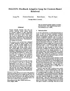
Fig. 1. (a) An example showing five consistent rectangles. The number at the top-right corner of each rectangle gives its color (action). A point that lies in both rectangles 1 and 3 receives the color 3, corresponding to the more specific match. A point lying in rectangle 4 gets the color 4. (b) An example of two inconsistent rectangles.

corresponds to the closed interval [1010 · · · 0, 1011 · · · 1]. The prefix ranges have the property that either two ranges are disjoint, or one contains the other. The range of s1 contains the range of s2 precisely when s1 is a prefix of s2 . For instance, the range of 10∗ is a superset of the range of 10110∗, but the ranges of 1010∗ and 110∗ are disjoint. A packet header has fully specified source and destination addresses, and thus corresponds to a point in the two-dimensional space. A filter (s, d) corresponds to the rectangle whose projections are the ranges of s and d in their respective dimensions. We denote this rectangle by R(s, d)—the points of R(s, d) are precisely the packet headers that match the filter (s, d). To emphasize that we are dealing with special rectangles, we use the term prefix rectangle. A prefix rectangle is a cross product of two prefix ranges. We say that two prefix rectangles are consistent if they are either disjoint or nested. The filter table D is consistent if every pair of its entries is consistent. Figure 1 shows examples of consistent and inconsistent rectangles. Consider a routing table D with N filter entries. These filters map to N prefix rectangles in the two-dimensional space [0, 2w − 1] × [0, 2w − 1]. We let each distinct action, associated with our filters, be represented by a color, where colors are integers numbered from one to K . Thus, we can think of a filter tuple (s, d), actioni as a prefix rectangle with color i. Since each packet must be classified into some filter, we assume, without loss of generality, that the prefix rectangles of D completely cover the two-dimensional space [0, 2w − 1] × [0, 2w − 1]. The filter classification induced by D is the mapping from packet headers (points) to the set of colors. Using the best matching filter rule, each packet header receives a unique color: the color assigned to a point is the color of the smallest (most specific) rectangle containing the point. (Refer to Figure 1.) We can now formulate the filter compression problem. Given N prefix rectangles with colors in {1, 2, . . . , K }, determine the smallest set of consistent prefix rectangles and their colors that induce the same coloring as the input set. Figure 2 shows an example. We begin by considering the problem in one dimension to help us develop the main idea for our algorithm.


3 1

291

1

1 2

2 3

3

2

3

3 2

2 (ii)

(i)

Fig. 2. An example of filter compression. (i) An input with eight rectangles, and (ii) an optimal solution using five consistent, prefix rectangles.

3. Compression in One Dimension. Consider a set of N prefixes D = {s1 , s2 , . . . , sn }, where each si is a binary bit string of length at most w, and the ith string is assigned color ci , with ci ∈ {1, 2, . . . , K }. Each string si corresponds to a contiguous interval on the line [0, 2w − 1], which we call the prefix range of si , and denote by R(si ). The set of N prefix ranges partitions the line [0, 2w − 1] into at most 2N − 1 “elementary intervals,” where each elementary interval is the interval between two consecutive range endpoints. Assign to each elementary interval the color of the smallest range containing that interval. Under this coloring rule, the prefix set D is a mapping from the points of the line [0, 2w − 1] to the color set {1, 2, . . . , K }. Given a point P, we let D(P) denote the color assigned to P by the set D. Figure 3 shows an example, where a set of prefixes partition the line into six elementary intervals. The colors assigned to these intervals, in left to right order, are 2, 1, 2, 3, 2, 3. (Our problem can also be formulated in the setting of a balanced binary tree of depth w: each address is a leaf, and a prefix is a internal node. In two dimensions the problem deals with a product of two binary trees, one for each dimension. We have chosen the geometric language of intervals and rectangles, however, because we find it more intuitive.) We say that two prefix sets D and D are equivalent if they induce the same coloring on the line [0, 2w − 1]. That is, D(P) = D (P), for all P ∈ [0, 2w − 1]. The onedimensional prefix compression problem can be formulated as follows: given a set of prefixes D, find the smallest prefix set D that is equivalent to D. Figure 3(ii) shows the optimal solution for the example in (i); the number next to each prefix range is its color. Our algorithm uses dynamic programming to compute the optimal set D . We divide a prefix range into halves, and then try to combine their optimal solutions. One difficulty with this obvious approach is that the combined cost may depend on the actual subproblem solutions. Consider, for instance, the case where we have four equal-length elementary intervals colored 1, 2, 3, 1. The left half subproblem has an optimal solution

2

2 3 1

2 3

(i)

1

3

3

2 (ii)

Fig. 3. An example of compression in one dimension. (i) An input with six prefix ranges, and (ii) an optimal solution using four prefix ranges.

292


{1, 2}; the right half subproblem has an optimal solution {3, 1}. However, adding them together does not give the optimal solution. (The optimal solution consists of only three prefixes, one each of colors 2, 3, and one with color 1 corresponding to the entire range.) With this motivation, we introduce the concept of a background prefix. Consider a prefix s, and its range R(s) ⊆ [0, 2w − 1]. Suppose we just want to solve the coloring subproblem for the range R(s). We say that a solution G for R(s) contains a background prefix if s ∈ G; that is, one of the prefix ranges in G is the whole interval R(s). The background color of G is the color of the background prefix. Figure 3(ii) shows an example that has a background prefix with color 2, while the set of prefixes in Figure 3(i) does not contain a background prefix. Our dynamic programming algorithm uses the key observation that it is sufficient to consider solutions in which background colors are well-defined. LEMMA 3.1. Every solution of the prefix compression problem in the range R(s) can be modified into a solution of equal cost with a background prefix. PROOF. Consider a solution without a background prefix. Pick a prefix p in this solution such that the range R( p) is not contained in any other prefix’s range. Replace p by s, and give it p’s color. 3.1. The Dynamic Programming Algorithm. We are given a set D = {s1 , s2 , . . . , sn } of N prefixes, where each si is a binary bit string of maximum length w, and the ith string is assigned color ci , with ci ∈ {1, 2, . . . , K }. Consider the coloring induced by D on the line [0, 2w − 1]: a point has the color of the smallest prefix range in which it lies. (Note that the fewer the bits in a prefix si , the longer the corresponding range R(si ) is. The null string ∗ corresponds to the whole range [0, 2w − 1], while a full w-bit string maps to a point.) We start by building a partition of [0, 2w − 1] in which each piece is monochromatic and each interval has length a binary power. That is, we recursively divide the line [0, 2w − 1] into halves until each piece is monochromatic. Because D has N prefixes, and each prefix has at most w bits, our final subdivision has size at most wN. Let p1 , p2 , . . . , p M , where M ≤ wN, denote the prefixes that correspond to the monochromatic intervals in the final subdivision. We call the R( pi )’s monochromatic binary intervals. These intervals are the basic subproblems for our dynamic program’s initialization. Given an arbitrary prefix range R(s) ⊆ [0, 2w − 1], and a color c ∈ {1, 2, . . . , K }, we define cost(s, c) = size of a minimal prefix set for R(s) with background color c. We initialize this cost function for the monochromatic binary intervals R( pi ) as follows. Let ci be the color of the interval R( pi )—that is, ci is the color induced on R( pi ) by the input prefix set D. Then, for each prefix pi , i = 1, 2, . . . , M, we set cost( pi , ci ) = 1 and cost( pi , c) = ∞ for all c = ci . The following lemma gives the general formula for this cost function. Given a prefix s, we use s0 and s1 to denote strings obtained by appending to s a 0 and a 1, respectively.


LEMMA 3.2.

293

For any prefix s and any color c,

cost(s, c) = min(cost(s0, c0 ) + cost(s1, c1 ) + 1 − [c = c0 ] − [c = c1 ]), c0 ,c1

where [x = y] evaluates to 1 if the predicate inside the brackets is true, and 0 otherwise. PROOF. Consider each of the four cases, depending on the outcome of predicates [c = c0 ] and [c = c1 ]. If the background colors for the two subproblems are the same as c (c = c0 = c1 ), then we can remove one of those prefixes from the combined solution. If the background colors are different (c0 = c1 ), but one of them, say c0 , is the same as c, then we extend the prefix corresponding to c0 to be the background prefix of the whole problem; if neither background color is the same as c, we introduce a new prefix corresponding to s and color it c. The optimal solution for (s, c) is obtained by picking the combination that gives the smallest number of prefixes. This completes the proof. If the input D has N prefixes, the number of colors is K , and the prefixes are w bits long, then the dynamic program based on Lemma 3.2 takes O(NKw) time and space. When we implemented our algorithm, we found that the worst-case memory requirement for this algorithm was infeasibly large to be of practical value. For instance, for the practical values of interest N = 50,000, w = 32, and K = 256, the dynamic program needs to construct a table of size 4 × 108 . Even assuming that each entry takes just 1 word of memory, the worst-case memory requirement for this algorithm is 3200 MB of memory! This motivated us to look for an improved algorithm, which we describe in the next section. Not only does the new algorithm require significantly less memory in practice, but it is also simpler and faster in practice. 3.2. An Improved Dynamic Program. Intuitively, maintaining K distinct solutions, one for each background color, for every subproblem seems like an overkill. (If we were only interested in the value of the solution, then we could of course choose not to store the intermediate solutions. However, they are needed for constructing the optimal prefix set.) Yet, as we saw earlier, keeping just one optimal solution does not work. However, we show below that storing just the background colors that give the smallest cost for each subproblem suffices. Given a prefix s, define cost(s) = minc cost(s, c). We define L(s) to be the list of background colors that give the minimum cost solutions for R(s): L(s) = {c | cost(s, ci ) = cost(s)}. Again, we initialize these lists for the monochromatic binary intervals by setting L( p) = {c( p)}. The following lemma shows how to compute these lists in a bottomup merge. (Recall that s0 and s1 are prefixes obtained by appending 0 and 1 to the prefix s.) LEMMA 3.3.

Suppose s is an arbitrary prefix. Then, L(s0) ∩ L(s1) if L(s0) ∩ L(s1) = ∅, L(s) = L(s0) ∪ L(s1) otherwise.

294


PROOF. We first consider the case L(s0)∩L(s1) = ∅. Since all colors in the intersection set L(s0) ∩ L(s1) are equivalent, it would suffice to show that cost(s, c) < cost(s, c) ¯ whenever c ∈ L(s0) ∩ L(s1) and c¯ ∈ L(s0) ∩ L(s1). It is easy to see that cost(s, c) = cost(s0, c) + cost(s1, c) − 1. (That is, the minimum is achieved by the first term in the expression of Lemma 3.2.) Assume, without loss of generality, that c¯ ∈ L(s0). Then we must have cost(s0, c) ¯ ≥ 1 + cost(s0, c), and cost(s1, c) ¯ ≥ cost(s1, c); if c¯ ∈ L(s1), the second inequality is strict. Now, it is easy to check that cost(s0, c) ¯ + cost(s1, c) ¯ − 1, cost(s, c) ¯ = min cost(s0, c) + cost(s1, c). ¯ Since cost(s0, c) ¯ ≥ 1 + cost(s0, c), and cost(s1, c) ¯ ≥ cost(s1, c), it follows that cost(s, c) ¯ ≥ cost(s0, c) + cost(s1, c) > cost(s, c), which proves the claim. Next, consider the case L(s0) ∩ L(s1) = ∅. In this case we show that cost(s, c) < cost(s, c) ¯ whenever c ∈ L(s0)∪L(s1) and c¯ ∈ L(s0)∪L(s1). We assume that c ∈ L(s0), and thus c ∈ L(s1). Then cost(s, c) = cost(s0, c) + cost(s1, c ), for any c ∈ L(s1). Now, since c¯ ∈ L(s0)∪L(s1), we have cost(s0, c) ¯ ≥ 1+cost(s0, c), and cost(s1, c) ¯ ≥ 1 + cost(s1, c ). Since  ¯ + cost(s1, c) ¯ − 1,  cost(s0, c) ¯ + cost(s1, c ), cost(s, c) ¯ = min cost(s0, c)   cost(s0, c) + cost(s1, c), ¯ it follows that cost(s, c) ¯ ≥ 1 + cost(s0, c) + cost(s1, c ) > cost(s, c), which completes the proof. Lemma 3.3 gives a straightforward dynamic programming algorithm. Starting from the initial color lists of the monochromatic binary intervals, the algorithm computes the lists for increasing longer prefix ranges. When computing the list for prefix s, we set L(s) = L(s0) ∩ L(s1) if L(s0) ∩ L(s1) = ∅; otherwise L(s) = L(s0) ∪ L(s1). Once all the lists have been computed, we can determine an optimal color assignment by a top-down traversal, as follows. We initialize the output list to root prefix s, and give it the background color c, for any c ∈ L(s). By construction, one or both of L(s0) and L(s1) contain c. If c ∈ L(s0) but c ∈ L(s1), then add to the output list prefix s1 with any color c ∈ L(s1). Recurse on L(s0) with background color c, and L(s1) with background color c . Similarly, if c ∈ L(s1) but c ∈ L(s0), add a new prefix s0 with any color c ∈ L(s0), and recurse on L(s0) with background color c and L(s1) with background color c. Otherwise c ∈ L(s0) ∩ L(s1), and we recurse on both L(s0) and L(s1) with background color c. The worst-case time and space complexity of the entire algorithm is O(NKw), since there are O(Nw) subproblems, and the size of a color list is at most K . Thus, from


295

a worst-case point of view, the dynamic program based on Lemma 3.3 is not much better than that of Lemma 3.2. However, in practice we found that the list sizes were much smaller than the total number of colors, and thus the memory requirement was substantially improved. See our experimental results in Section 5. We next describe our main result: the dynamic programming algorithm for filter compression.

4. Optimal Filter Compression. Consider a consistent set D of N filters. Each filter (s, d) corresponds to a rectangle R(s, d) in the two-dimensional space [0, 2w − 1] × [0, 2w − 1]. The color of R(s, d) is the color (action) associated with filter (s, d). Using the best matching filter rule, the set D gives a mapping from the set of points [0, 2w − 1] × [0, 2w − 1] to the set of colors. Let D(P) denote the color assigned to point P by D. Geometrically, D(P) is the color of the smallest rectangle containing P. (We assume that the set of rectangles cover the domain [0, 2w − 1] × [0, 2w − 1]. This can be enforced by adding a default filter.) Our goal is to find the smallest consistent set of filters D that realizes the same coloring map as D; that is, D(P) = D (P) for all points P. Our algorithm generalizes the dynamic program of the preceding section. We start with the observation that any solution can be modified to contain a background filter. We say that a solution D for the rectangle R(s, d) contains the background filter if (s, d) ∈ D. The background color of D is the color assigned to the filter (s, d). Figure 2(ii) shows an example that has a background filter of color 1; the set of filters in Figure 2(i) does not contain a background filter. The following generalizes the background prefix lemma. LEMMA 4.1. Every solution of the filter compression problem in a prefix rectangle R(s, d) can be modified into a solution of equal cost with a background filter. PROOF. The proof is identical to the proof of Lemma 3.1. Consider a solution without a background filter. We pick a rectangle r in this solution that is not contained in any other rectangle. Replace r by the background rectangle R(s, d), and give it r ’s color. It is easy to check that this modification does not alter the routing table’s behavior. Given a prefix rectangle R(s, d), and a color c ∈ {1, 2, . . . , K }, define cost(s, d, c) = size of a minimal filter set for R(s, d) with background color c. The following lemma gives the general formula for this cost function. (Recall that we use the notation x0 (resp. x1) to denote the bit string x with 0 (resp. 1) appended.) Before we state and prove this lemma, we need one more definition. We say that a prefix rectangle R = (s , d ) spans R(s, d) along the s-axis (resp. d-axis) if s = s and d is a prefix of d (resp. d = d and s is a prefix of s ). Figure 4 illustrates this definition. LEMMA 4.2.

For any rectangle R(s, d) and any color c, cost(s, d, c) = min{costv (s, d, c), costh (s, d, c)},

296


s0

s1

G

d1

d d0

F

s Fig. 4. F spans R(s, d) along the s-axis; G spans it along the d-axis.

where costv (s, d, c) = min(cost(s0, d, c0 ) + cost(s1, d, c1 ) + 1 − [c = c0 ] − [c = c1 ]) c0 ,c1

and costh (s, d, c) = min(cost(s, d0, c0 ) + cost(s, d1, c1 ) + 1 − [c = c0 ] − [c = c1 ]). c0 ,c1

PROOF. The proof is similar to the proof of Lemma 3.2. No consistent solution can contain rectangles spanning R(s, d) in both directions. If an optimal solution with background color c has no rectangle spanning R(s, d) along the s-axis, then we can split it into left and right subsolutions exactly as in the one-dimensional case, and its cost will be costv (s, d, c). Similarly, if an optimal solution has no rectangle spanning R(s, d) along the d-axis, then we can split it into top and bottom subsolutions, and its cost will be costh (s, d, c). This completes the proof. 4.1. An Improved Algorithm. As in the one-dimensional case, the dynamic program of Lemma 4.2 can be improved in practice (though not in the worst case) by maintaining the list of only those background colors that give optimal solutions. Define cost(s, d) = minc cost(s, d, c). Let L(s, d) denote the list of colors that achieve minimum cost for the coloring subproblem R(s, d): L(s, d) = {c | cost(s, d, c) = cost(s, d)}. In the following we refer to the elements of D as input rectangles. Define Lh (s, d) to be the set of background colors that allow an optimal solution that splits R(s, d) horizontally. Similarly, define Lv (s, d) to be the set of background colors that allow an optimal solution that splits R(s, d) vertically. We define costh (s, d) and costv (s, d) as the costs of these solutions.


297

FILTERCOMPRESS (s, d, D) 1. (∗ All background colors are equally good. ∗) If no rectangle in D lies entirely inside R(s, d), then set L(s, d) = {c}, where c is the color of rectangle R(s, d); set cost(s, d) = 1, and return. 2. (∗ Compute the cost of a vertical split. ∗) Set costv (s, d) = ∞. If no rectangle in D spans R(s, d) along the s-axis, then FILTERCOMPRESS (s0, d, D) FILTERCOMPRESS (s1, d, D) if L(s0, d) ∩ L(s1, d) = ∅ then Lv (s, d) = L(s0, d) ∩ L(s1, d) costv (s, d) = cost(s0, d) + cost(s1, d) − 1 else Lv (s, d) = L(s0, d) ∪ L(s1, d) costv (s, d) = cost(s0, d) + cost(s1, d) 3. (∗ Compute the cost of a horizontal split. ∗) In this case we compute Lh (s, d) and costh (s, d) exactly as the step above. 4. (∗ Take the cheaper of the two splits. ∗) if costv (s, d) > costh (s, d) then cost(s, d) = costh (s, d) L(s, d) = Lh (s, d) else if costv (s, d) < costh (s, d) then cost(s, d) = costv (s, d) L(s, d) = Lv (s, d) else cost(s, d) = costv (s, d) L(s, d) = Lh (s, d) ∪ Lv (s, d) The initial call to our algorithm is FILTERCOMPRESS (∗, ∗, D), where ∗ is the empty prefix. We now argue the correctness of the algorithm. The base case of the algorithm occurs when every point in R(s, d) is assigned the same color. In this case our algorithm simply returns the single filter for that rectangle. Steps 2 and 3, respectively, deal with cases when the optimal solution has a vertical split or a horizontal split. Since a consistent optimal solution cannot have rectangles spanning R(s, d) both horizontally as well as vertically, at least one of these two cases must occur. The algorithm in each of these cases is just the one-dimensional prefix compression algorithm, which we discussed in Section 4.1. Finally, in Step 4, we choose the better of the two solutions found by the vertical or the horizontal splits. Next, we analyze the running time of the algorithm. As is the standard practice with dynamic programming algorithms, we tabulate the solutions to the subproblems, so we do not solve the same subproblem over and over again. We assume the reader is familiar with this memoization; an interested reader may refer to the textbook by Cormen et al. [5] for details. A subproblem FILTERCOMPRESS (s, d, D) makes a recursive call only if R(s, d) contains at least one input rectangle of D inside it. The total number of subproblems is

298


O(Nw); the cost of deciding if a rectangular region is spanned by some filter is O(w); and the cost of maintaining color lists per subproblem is O(K ). Thus, the total time and space complexity of the algorithm is O(NKw2 ) in the worst case. THEOREM 4.3. Given a consistent set of N filters, with K distinct colors and at most w-bit prefixes, we can compute an optimal filter compression in O(NKw2 ) worst case time.

5. Extensions and Experimental Results 5.1. Minimizing the Bit Complexity. We have used the number of filters as our complexity measure. Instead one could ask to minimize the total bit complexity of the routing table. Algorithms that use tries or bit vectors for filter classification [2], [7], [12], [15] are sensitive to the total number of bits in the routing database. Given a filter f = (s, d), let b( f ) denote the bit length of s plus the bit length of d. Then the bit complexity of a n routing table D = { f 1 , f 2 , . . . , f n } is i=1 b( f i ). We could ask for a routing table of minimum bit complexity that is equivalent to D. Our algorithms are easily modified to optimize the bit complexity of the routing table: instead of counting 1 for each filter, count its number of bits. 5.2. Experimental Results. We implemented our dynamic programming algorithms, for both one- and two-dimensional compression. The algorithms were implemented in C++ on a 300 MHz Pentium II running Windows NT. We do not have any publicly available filter databases to test our two-dimensional algorithm, since stateful routers are still in their infancy. On the other hand, prefix tables are widely available for large backbone routers, so we were able to test our one-dimensional compression algorithm. We ran our algorithm on three publicly available routing tables, obtained from the MaeEast Exchange Point [13]. The number of prefixes in these databases varied from about 8000 (Paix) to about 41,000 (Mae-East). The total number of colors (distinct next hops) varied from 17 to 58. Table 1 shows our results. While one-dimensional results are no indication of the two-dimensional problem, it should be encouraging that our prefix compression algorithm achieves compression of 30–40% even in these highly aggregated prefix tables. It therefore appears likely that significant compression might be possible in the routing tables, which are going to be automatically generated. Table 1. One-dimensional prefix compression.∗ Database

Input

Output

Reduction (%)

Memory (MB)

Time (s)

Mae-East PacBell Paix

41,455 24,728 7,982

23,680 14,168 5,888

42 42 26

3.8 2.1 0.8

2.73 1.85 0.72

∗ The input and output are the number of prefixes. The maximum prefix length was w

and the number of colors varied between 17 and 58.

= 32


299

6. Concluding Remarks and Open Problems. We gave an efficient algorithm for computing an optimal filter compression for reducing state information in IP routers. The algorithm is relatively simple, and exploits some basic geometric properties of consistent prefix rectangles in two dimensions. The basic dynamic programming algorithm runs in O(NKw2 ) worst-case time, for N filters with K colors and w bit prefixes. While the improved dynamic program does not reduce the worst-case complexity, it should be substantially better in practice. IP routers certainly need to move beyond the current best-effort service model, if they are to be used for advanced services like audio, video, or IP telephony. Past history has shown that highly stateful solutions like ATM (asynchronous transfer mode) have failed to be widely adopted despite their ability to provide quality of service. Achieving similar capabilities in IP routers with minimal per-filter state appears to be the most promising alternative. Our hope is that algorithms like ours for filter compression will make stateful routers more scalable, and thus more acceptable. Several open problems are suggested by our work. First, our approach requires the routing table to be consistent (or, in networking parlance, conflict-free)—that is, if two filters overlap, then one contains the other. Arbitrary prefix filters may not satisfy this restriction. In order to define the effect of an inconsistent routing table unambiguously, we need to assign priorities to filters, and choose the matching filter with the highest priority. This leads to the following geometric problem. Consider a set T of n prefix rectangles, defined over a discrete domain U , each with a height and a color. Each point of U is assigned the color that is visible from z = ∞. We say that another set of rectangles is equivalent to T if it gives the same color assignment on U . Develop an efficient algorithm to find the smallest set of rectangles equivalent to T . Our approach does not seem to work for this problem. Second, our algorithm does not extend to more than two dimensions. The main difficulty is that even if (three-dimensional) rectangles are consistent, they cannot always be separated using a plane split. Thus, there does not appear to be a small set of subproblems whose solutions can be combined into larger solutions for the dynamic program. It is an open problem whether the compression problem for routing tables with three or more attributes is NP-Complete.

Acknowledgment. We thank the referees for valuable comments and suggestions that have significantly improved the presentation of our paper.

References [1] [2] [3] [4] [5]

H. Adiseshu, S. Suri, and G. Parulkar. Detecting and Resolving Packet Filter Conflicts. Proc. of IEEE INFOCOM 2000, pp. 1203–1212, Tel Aviv, March 2000. A. Brodnik, S. Carlsson, M. Degermark, and S. Pink. Small Forwarding Table for Fast Routing Lookups. Proc. ACM SIGCOMM, pp. 3–14, September 1997. D. B. Chapman and E. D. Zwicky. Building Internet Firewalls. O’Reilly, Cambridge, MA, 1995. W. Cheswick and S. Bellovin. Firewalls and Internet Security. Addison-Wesley, Reading, MA, 1995. T. Cormen, C. Leiserson, and R. Rivest. Introduction to Algorithms. MIT Press, Cambridge, MA, 1990.

300


[6]

R. Daves, C. King, S. Venkatachary, and B. Zill. Constructing Optimal IP Routing Tables. Proc. of IEEE INFOCOM 1999, pp. 88–97, 1999. D. Decasper, Z. Dittia, G. Parulkar, and B. Plattner. Router Plugins: A Software Architecture for Next Generation Routers. IEEE/ACM Transactions on Networking, February 2000. A. Demers, S. Keshav, and S. Shenker. Analysis and Simulation of a Fair Queueing Algorithm. Journal of Internetworking Research and Experience, pp. 3–26, 1990. D. Eppstein and S. Muthukrishnan. Internet Packet Filter Management and Rectangle Geometry. Proc. of 12th ACM–SIAM Symp. Discrete Algorithms, pp. 827–835, 2001. A. Feldmann and S. Muthukrishnan. Tradeoffs for Packet Classification. Proc. of IEEE INFOCOM 2000, Tel Aviv, March 2000. M. R. Garey and D. S. Johnson. Computers and Intractability: A Guide to the Theory of NPCompleteness. Freeman, New York, 1979. T. V. Lakshman and D. Stidialis. High Speed Policy-based Packet Forwarding Using Efficient MultiDimensional Range Matching. Proc. of ACM SIGCOMM, 1998. Merit, Inc. ftp://ftp.merit.edu/statistics/ipma. Routing Table Snapshot, 14 Jan. 1999, Mae-East NAP. V. Srinivasan and G. Varghese. Faster IP Lookups Using Controlled Prefix Expansion. Proc. of Sigmetrics ’98, 1998. V. Srinivasan, G. Varghese, S. Suri, and M. Waldvogel. Fast Scalable Level Four Switching. Proc. of ACM SIGCOMM, 1998. V. Srinivasan, S. Suri, and G. Varghese. Packet Classification Using Tuple Space Search. Proc. of ACM SIGCOMM, 1999. M. Waldvogel, G. Varghese, J. Turner, and B. Plattner. Scalable High Speed IP Routing Lookups. Proc. of ACM SIGCOMM, 1997.

[7] [8] [9] [10] [11] [12] [13] [14] [15] [16] [17]