[6]) is used to compute the frequency of an orbit in the 2D phase space. ... Figure 1: Tune error (N) versus N for APA and Fitted .... of the FFT plus Hanning filter.
ALGORITHMS FOR A PRECISE DETERMINATION OF THE BETATRON TUNE � R.Bartolini, M.Giovannozzi, W.Scandale CERN, Geneva, Switzerland A.Bazzani, Dip. di Matematica-Bologna E.Todesco, INFN-Bologna 1 INTRODUCTION In circular accelerators the precise knowledge of the betatron tune is of paramount importance both for routine operation and for theoretical investigations. The tune is measured by sampling the transverse position of the beam for N turns and by performing the FFT of the stored data. One can also evaluate it by computing the Average Phase Advance (APA) over N turns. These approaches have an intrinsic error proportional to =N . However, there are special cases where either a better precision or a faster measurement is desired. More efficient algorithms can be used, as those suggested by E. Asseo [1] and recently by J. Laskar [2]. They provide tune estimates by far more precise than those of a plain FFT, as discussed in Ref. [3]. Another important issue is the effect of the finite resolution of the instrumentation used to measure the beam position. This introduces a noise and the frequency response of the beam is modified [4, 5] thus reducing the precision by which the tune is determined. In Section 2 we recall the methods based on the APA approach. In Section 3 we introduce the FFT based methods and the estimate of the algorithmic error as a function of N . In Section 4 we discuss the effect of noise.
1
2
APA TECHNIQUES
APA The APA method (see for instance Ref. [6]) is used to compute the frequency of an orbit in the 2D phase space. Given a 2D orbit n with n ; :::; N , the tune is given by the average value of �n :
x( )
=1
N
�APA (N ) = 2�(N1 1) �n ; (1) n=2 where x(n) = (x(n); px (n)) and �n is the phase advance between the iterate n 1 and the iterate n. The accuracy X
(see Ref. [3]) in the tune estimation is given by
j�APA (N )j � CAPA N :
(2)
where CAPA is a numerical constant. This estimate holds provided the betatron tune is separated by any other spectral lines by at least =N .
1
� Work partially supported by EC Human Capital and Mobility contract Nr. ERBCHRXCT940480
Fitted APA A fitting procedure can improve the convergence of the APA method. In general the value of �APA N performs damped oscillations around the asymptotic value of �0 corresponding to the non–linear tune. To get rid of the periodic component in �APA N we introduce the averaged tune, i.e.
( )
( )
< �APA (n) >= n 1 1
=2
n
X
m=2
�APA (m)
(3)
where n ; :::; N . This quantity converges to �0 asymptotically. Therefore one can give a better estimate by fitting the averaged APA with a linear regression
< �APA (n) >� �Afit(N ) + n A 1
=2
(4)
( )
where n ; :::; N .�Afit N is the estimated value of �0 and A is a constant. Computer simulations performed with several accelerator models show that the accuracy of this method is: j�Afit N j � CAfit (5) 2 :
( )
N
where CAfit is a numerical constant. In Fig. 1 we show the behaviour of the error on the tune determination with APA and fitted APA starting from a signal made of two main frequencies plus harmonics, given by
z (n) =
X
k
ak e2�i�0 kn +
1 N = 0 31
X
k
bk e2�i�1 kn
(6)
where jak j; jbkj < , n 2 . In our simulations we chose �0 : and �1 : to simulate the working point of the LHC. Five harmonics of �0 and �1 with exponentially decreasing amplitudes are considered.
= 0 28
3
FFT TECHNIQUES
Using N values of the transverse position one can find the tune by inspecting the power spectrum computed by an FFT and choosing the value corresponding to the maximum frequency response. There are methods to improve the resolution of the spectral analysis which rely on the assumption that the spectrum of the transverse oscillations of the beam contains a limited number of peaks. The peaks correspond to the eigenfrequencies of the motion or to combinations of them driven by either linear or non-linear coupling or by the interplay of synchrotron and betatron motion. In general, the harmonics of these peaks decrease very rapidly, and therefore can be neglected.
This estimate holds, provided the distance in frequency between the main peak and any other peak of the spectrum is larger than =N (see Ref. [3]). For N � , (10) is well approximated by
0
1
(a)
-2
Log |ε(N)|
-4
1
� )j � �Fint = Nk + N1 j�(� j)�j(+�kj+1 �(�k+1)j k
-6 -8 -10
(12)
which is the formula given by Asseo in [1].
-12 -14
APA Fitted APA
-16 -18
1.00
1.50
2.00
2.50
3.00
3.50
4.00
4.50
5.00
Log N
(N ) versus N for APA and Fitted
Interpolated FFT with data windowing A standard approach to improve the accuracy of Fourier analysis is based on time window filters: the data z n are weighted with functions � n (see Ref. [7]). In this case, the Fourier coefficients of the orbit read
Figure 1: Tune error � APA for the signal (6)
(1) (2)
( )
FFT The time series fz ; z ; :::; z N g made of N consecutive values of the orbit coordinates, can be expanded as a linear combination of N orthonormal functions:
z (n) =
N
X
j =1
�(�j ) exp(2�in�j )
�j = Nj ;
(7)
()
( )
=2
CFFT = 12 :
Interpolated FFT Since the error in the FFT estimate is due to the discreteness of the spectrum, one can obtain better results by interpolating the shape of the spectrum around the main peak. The tune is then the abscissa of the maximum of the interpolating function. We use as interpolating function the continuous spectrum of a pure sinusoidal signal with unknown frequency �Fint: N�(�Fint �j ) j�(�j )j = Nsinsin �(�Fint �j )
(9)
The formula for the tune reads
� )j sin( N� ) � �Fint = Nk + �1 atan j�(� j)�j (+�kj+1 �(�k+1)j cos( N� ) k
(10)
j�(�k)j being the peak of the FFT spectrum and j�(�k+1)j its highest neighbour. For large N , the error is given by
j�Fintj � CNFint 2 :
n
X
n=1
z (n)�(n) exp( 2�in�j )
(13)
If we consider Hanning-like filters of order l: � � �l (n) = Al sinl �n N
(14)
where Al is a normalization constant we obtain that the interpolated value of the tune, in the limit N � , reads
1
� k 1 ( l + 1) � ( � ) l n +1 �Fint = N + N �(� ) + �(� ) 2 (15) n n+1 For the Hanning filter, l = 2, the exact formula for the tune
reads:
�FHan = Nk + 21� arcsin sin 2N� �
(8)
M . The FFT provides a very fast estimate of where N the complete Fourier spectrum; however, the evaluation of the main frequency is made with a poor precision.
�(�j ) = N1
�
One assumes that the N samples z n are in fact extended in a periodic sampled signal of period N . The Fourier coefficients � �j are usually evaluated with the Fast Fourier Transform algorithms. The error associated is due to the discreteness of the frequencies �j , and is given by
j�FFT j � CFFT N
()
()
(11)
�
(16)
where
= A j�(�k)j; j�(�k+1)j; cos 2N� �
and the function A is given by
�
(17)
p
+b � A(a; b; c) = (a +a2bc+)(ba2 + b2)abc
(18)
� reads � = c2(a + b)2 2ab(2c2 c 1)a2 + b2 + 2abc (19)
where
The details are given in Ref. [3]. The effect of the filter is to change the interpolating function (9) as to increase the width of the main peak centered at �Fint and to decrease the amplitude of the sidelobes. In fact the height of the lobes becomes proportional to =N l+1 instead of =N . The tune error is: j�Fintj � CFHan (20) l+2
1
1
N
where CFHan is a numerical constant. Note that by increasing l the main peak of the interpolating function is broadened thus reducing the resolution of the algorithm. The filter (14) with l , is a satisfactory compromise
=2
0 -2
-4
-4
Log |ε(N)|
Log |ε(N)|
0 -2
-6 -8 -10
FFT FFT Interpolated
-12
FFT + sin^2 filter Interpolated
-6 No noise
-8
S/N=1000 -10
S/N=100
-12
S/N=10 S/N=1
FFT + sin^4 filter Interpolated
-14
-14
-16 0
1
2
3
4
-16
5
0
1
2
Log (N)
3
4
5
Log(N)
(N ) versus N for different methods
Figure 2: Tune error � for the signal (6)
( )
Figure 4: Tune error � N versus N for different values of the signal over noise power ratio s=n. The signal is given by equation (21). The tune is computed using the interpolation of the FFT plus Hanning filter.
0 -2
domain this introduces a white noise component whose r.m.s. amplitude is = LSB. The effect on the tune precision can be investigated using a simple numerical model that contains a sinusoidal signal of the type (6) plus a white noise component of the form
12
Log|ε(N)|
-4 -6 -8 -10
� (n) = z (n) + r(n)LSB;
APA
-12
FFT FFT interpolated + Hanning
-14
()
FT + Hanning
-16
1
2
3
4
5
Log N
(N ) versus N for different methods (x; 0; x; 0) at half dynamic aperture
Figure 3: Tune error � for an initial condition of the CERN SPS
in many different applications. Various interpolation techniques are compared in Fig. 2 on the model given by eq. (6). The interpolated FFT associated with the Hanning filter performs extremely well and is recommended as the best approach. Similar results are found with more realistic accelerator models and with experimental data obtained at the CERN SPS and LEP [3, 8]. In Fig. 3 the behaviour of � N for the SPS model is shown.
( )
4
(21)
EFFECT OF NOISE
Several perturbing effects can reduce the precision by which one measures the transverse beam position. The main source of uncertainty is related to the Analog-toDigital-Converter (ADC), used to digitize the position signal that overcomes all the other perturbations like the non-linear response of the pick-up, its finite resolution, the electronic noise, the distortion due to the cable transmission, and so on. The least significant bit (LSB) of the ADC is equal to zero or one, randomly. In the frequency
where r n is a random variable equal to 0 or 1. The reference case, without noise, is compared to several cases, where the signal to noise power ratio (s=n) vary over a wide range. The precision by which the tune can be identified is reduced, as shown in Fig. 4. In particular, the beneficial effect of the Hanning filter is completely lost, even though the noise is small (s=n ). Similar results hold for the other Hanning-like filters. On the other hand, the effect of the noise has a weak dependence on the s=n ratio. Furthermore, the tune error scales always better than =N , even in the extreme case when the noise and the signal powers are equal [9]
= 1000
1
5
REFERENCES
[1] E. Asseo, CERN PS/85–3 (LEA), (1985). [2] J. Laskar, Physica D 67, 1993, pp 257–281. [3] R. Bartolini et al., CERN SL/95–84 (AP), (1995) and Part. Acc., in press. [4] H. Jacob et al. CERN SL/95-68 (BI), (1995). [5] H. J. Schmickler, CERN LEP Note (BI)/87–10, (1987). [6] A. Bazzani et al., CERN 94/02, (1994) [7] F. J. Harris, Proceedings of the IEEE 66, 1978, pp 51–83. [8] R. Bartolini et al., CERN SL MD Note 207, (1996) [9] R. Bartolini et al., Proceedings of LHC 95, Montreux (1995) Part. Acc. in press.