Sep 21, 1988 - AT&T Bell Laboratories ... AT&T Technical Journal, Vol. 69, No. ..... However, since this search maintains no history of states, the search can not ...
Algorithms for Automated Protocol Validation Gerard J. Holzmann AT&T Bell Laboratories Murray Hill, New Jersey 07974
ABSTRACT This paper studies the four basic types of algorithm that, over the last ten years, have been developed for the automated validation of the logical consistency of data communication protocols. The algorithms are compared on memory usage, CPU time requirements, and the quality, or coverage, of the search for errors. It is shown that the best algorithm, according to above criteria, can be improved further in a significant way, by avoiding a known performance bottleneck. The algorithm derived in this manner works in a fixed size memory arena (it will never run out of memory), it is up to two orders of magnitude faster than the previous methods, and it has superior coverage of the state space when analyzing large protocol systems. The algorithm is the first for which the search efficiency (the number of states analyzed per second) does not depend of the size of the state space: there is no time penalty for analyzing very large state spaces. The effectiveness of the new algorithm is illustrated with the validation of a protocol of a realistic size: the ANSI/IEEE Standard 802.2 for logical link control.
AT&T Technical Journal, Vol. 69, No. 2, pp. 32−44.
Sep 21, 1988
Algorithms for Automated Protocol Validation Gerard J. Holzmann AT&T Bell Laboratories Murray Hill, New Jersey 07974
1. Introduction The analysis of communication protocols by the exhaustive inspection of reachable composite system states in a finite state machine model is a relatively straightforward and well−understood procedure. It would seem that for an exhaustive analysis we have to inspect at most a number of composite system states that is equal to the Cartesian product of the number of states in each independently executing entity of the protocol. Depending on the size of the original system, this may or may not be prohibitively expensive. There are, however, delicate trade−offs to be made that give us a choice of algorithms that may either inspect more or fewer system states than the limit stated above. The trade−offs are between the coverage, or the completeness, of the search and its CPU requirements in terms of run time and memory usage. In the comparison of search algorithms the following parameters are used. Table 1 — Parameters
__________________________________________________________________________________ ________________________________________________________________________________ Symbol Description Typical Value _________________________________________________________________________________ M bytes of memory available for the complete search 107 bytes R total number of reachable composite system states 108 states S bytes of memory required to store one state from R 102 bytes L average number of successor states per state in R 2 states E search efficiency: total CPU time required per state 10−2 seconds average length of one acyclic execution sequence 102 states _D________________________________________________________________________________
The last column gives an order of magnitude value for each parameter, assuming a medium size computer (e.g. a DEC/VAX−750) and a test protocol of a realistic size. Times are given in seconds, sizes are in bytes, and the length of an execution sequence is measured by the number of states it passes through. The values in Table 1 will be used for comparing the performance of search algorithms under realistic conditions. The value for M needs little justification: it is determined by available hardware. The values for S, R, L and D are conservative estimates based on measurements of a range of different protocols [Holzmann ’87a, ’88]. As one specific example, for the IEEE 802.2 logical link control protocol discussed in Section 7, the parameter values are: S = 150, R ∼ ∼2. 5, and D ∼ ∼10 3 . The value for E in Table 1 is an average ∼ 10 9 , L ∼ based on measurements of typical search algorithms, and matches the performance of at least one known, and generally available, implementation of a traditional algorithm [Holzmann ’85]. No lower (i.e. better) values for E have been reported in the literature, though not infrequently higher values are mistakenly published as improvements over existing methods [e.g. Vuong ’86, Kakuda ’88]. In Section 5.5 (Table 3) we will calculate the cost of the basic operations in a traditional search algorithm. That calculation also leads to the same value for E given in Table 1. The evaluation of search algorithms that follows is machine independent. Obviously, any algorithm will run faster on a bigger machine and slower on a PC. What we are interested in here is, however, the relative performance. Therefore all algorithms are compared for their performance on the same machine with one given set of constraints.
-2-
2. The Problem Figure 1 gives an overview of the protocol validation problem.
Implementation
Protocol Specification
Formal (FSM) Model
Validation Kernel
Figure 1 — Specification, Implementation, and Validation The original specification of a protocol is the result of design process and in its final form, for instance, as presented in a standards document such as [IEEE ’85]. The problem of verifying that an implementation of the protocol conforms to the original specification is a separate area of research that is outside the scope of this paper. The protocol validation problem considered here is the problem of verifying that the original specification is itself logically consistent. If, for instance, the specification has a design error, an implementation is expected to pass a conformance test if it contains the same error. The conformance test should fail only if implementation and specification differ. A validation for the logical consistency of the protocol, however, must reveal the design error. To verify logical consistency, a formal finite state machine (FSM) model of the protocol is constructed. The model will generally specify a set of asynchronous, communicating finite state machines. The model can contain interaction primitives, such as send and receive operations on finite message queues, or it can leave it to the model builder to construct primitives from simpler constructs. For the remainder of the paper it is irrelevant which particular constructs are used. The importance is only that the model defines behavior in terms of states and state transitions. The individual behavior of one of a set of asynchronous finite state machines in the model is defined by a finite set of local machine states and local state transitions. The local machine states will be called ‘process states.’ The system as a whole is defined, minimally, by the composite of all individual process states and the combination of all simultaneously enabled local state transitions. We will use the term ‘state’ as a short−hand for ‘composite system state’ from here on. Where this can cause confusion we will use the terms ‘process state’ or ‘system state.’ Given an initial state for each machine in the system, the sets of process states and system states can be divided into two disjoint classes: reachable states and unreachable states. Normally it is required that the model not contain any unreachable process states: they would correspond to unexecutable code in an implementation. Normally, also, the set of unreachable system states is several orders of magnitude larger than the set of reachable system states. The set of unreachable system states should include all error states. The formal model can be subjected to an exhaustive reachability analysis to determine which states are reachable and which are not. Every reachable state, and possibly every sequence of reachable states, can be checked for a given set of correctness criteria. These criteria can be general safeness conditions that must hold for any protocol, such as the absence of deadlocks or buffer overruns, or they can be protocol specific liveness requirements such as the proper working of a message retransmission discipline. As indicated in Figure 1, the task of building a finite state machine model can be separated from the task of performing the actual reachability analysis. In the effort to construct a tractable model we can exploit symmetries in the specification, apply reduction rules, and projection methods [Lam ’84]. For any given FSM model, big or small, smart or dumb, the reachability analysis task, however, is the same. This, then, is the topic of this paper: the problem of designing the fastest possible validation kernel for reachability analyses. 3. Search Algorithms We define four basic types of search algorithms. They are listed in decreasing order of memory usage. For each algorithm a sample implementation is given in pseudo−code. The first three algorithms require an initialization routine, which we will call init().
-3-
init() { W = { initial_state }; A = { }; }
/* work set: to be analyzed */ /* analyzed states */
The routine initializes two sets: a working set of system states to be analyzed, called W, and a larger set of analyzed states, called A. Set A is also referred to as the ‘system state space.’ Ideally, it will include all reachable system states R when the algorithm terminates. Type 1: Exhaustive Search. An unmodified exhaustive search strategy, also called a perturbation analysis, was one of the first methods tried for programming the reachability analysis [Zafiropulo ’77−78, Hajek ’78], and is still in use [e.g. Aggarwal ’83, Bourguet ’86, Rafiq ’83, Richier ’87, Sabnani ’86]. It attempts to build the complete system state space containing all reachable states R. If connectivity information also is stored it can be used for the detection and analysis of execution cycles [e.g. Sabnani ’86]. type_1() /* exhaustive search */ { while (W nonempty) { q = element from W; if (q is error_state) report_error(); else { for each successor state s of q if (s is not in A or W) add s to W; } delete q from W; add q to A; } }
Practical bounds to specifically the amount of available memory restrict the applicability of this type of search algorithm. These bounds can be quantified as follows. To make the comparison fair, it is assumed that no connectivity information is stored (only an algorithm of Type 1 can truly use this information in analyses). To include it in the formula below, replace every occurrence of S with S + B×L, with B the number of bytes required to store a link. Typically B = 4, the size of an address pointer on our reference machine. To complete a Type 1 algorithm we need S×R bytes of memory, or M ≥ S×R. The maximum number of states A that effectively can be analyzed then is: M A ≤ ___ S and this search will take E×M T ≥ _____ seconds. S For the values from Table 1 we have A ∼ ∼ 10 5 states
and
T ∼ ∼ 10 3 seconds.
It is therefore reasonable to analyze small to medium size protocols exhaustively with a Type 1 algorithm. Larger models are more challenging. Specifically, if A H. The hash function will then necessarily produce the same hash value for on the average A/H different states. All states that hash onto the same value are stored in a linked list, that is accessible via the lookup table under the calculated index (the hash value). On the average then, when the table is full, each new state must be compared to A/H other states, before it is either inserted into the linked list, or discarded as redundant. In a Type 1 or Type 2 algorithm, therefore, the following three operations must be performed for a new state: (1) calculating a hash value, (2) comparing the new state against a subset of the previously analyzed states already in the hashlist, and (3) inserting the new state into a linked list. Note carefully that these operations are not a peculiarity of a specific implementation but fundamental operations that are unavoidable in this type of search. The use of the hash table is an optimization technique that, in return for a small extra cost (1), avoids the worst case in (2) that would force us to compare each newly generated state against against all previously analyzed states before it can be discarded or inserted. Table 3 tabulates the minimal cost of each operation on our medium size reference machine. Calculating a hash value, for instance, minimally requires an amount of time that is linear in the number of bytes S in the state description. For a DEC/VAX−750 it takes approximately 10 − 6 seconds per byte. Table 3 – Cost of State Space Maintenance (Seconds)
__________________________________________________________________ ____________________________________________________________________ Number of Bytes Cost per Byte Typical Value Operation ___________________________________________________________________ Calculating the Hash S 10−6 10−4 −5 Comparing States 10 10−2 AxS/H Inserting New States S 10−5 10−3 ___________________________________________________________________
The most time consuming operation is comparing states. Its effect can be reduced by increasing H, but clearly there is another trade−off to be made here. ∼ 4 . The table itself takes up H×B bytes of memory, plus B bytes for each state A typical value for H is H ∼10 that is inserted. B is the size of a ‘link’ or ‘address pointer.’ On most machine B = 4, which means that a table with say 256,000 slots would require more than one Mbyte of overhead that can no longer be used to
-9-
store states. Since this is about 10% of the total amount of memory available for the search (Table 1), it is prudent to make H smaller. For typical values of H (10 4 ), S (10 2 ), and M (10 7 ), and with A growing from 1 to M / S states, we find a minimal cost (the sum of all three operations) increasing with A from approximately 10 − 3 to 10 − 2 seconds per state (cf. Table 1). This is again an optimistic estimate. Note that we disregarded all other operations that are required to perform the analysis of the states. The search efficiency E degrades as the search progresses: there is a growing time penalty for analyzing large systems. 6. Supertrace If we were able to avoid the last two operations from Table 3 completely, we would be able to speed up the search algorithm by a factor of 10×A / H, or by about two orders of magnitude. We can do this as follows. We use a very large value for H to reduce the number of hash conflicts. Here we will use H = 8×M, which for typical M makes H = O( 10 8 ), instead of O( 10 4 ). This hash value is now used to calculate the position of a single bit in the available memory arena M (there are eight bits per byte). A bit value of one will now be used to indicate that the state corresponding to this hash value has been previously analyzed. The state itself is not stored. Since no states are stored there are also no states to compare a new state against: the bit position uniquely identifies the state. Two things make this method work: the sparseness of the state space and the very large size of H. Both will make hash conflicts rare for all cases where A < H, and when A > H the hashing will effectively help us to reduce the coverage of the search to precisely the number of states that can analyzed within the given hardware constraints, that is O(10 8 ) states. The next two sections explain the storage method in more detail. It can be skipped on a first reading. Detailed Explanation If H can be chosen to be much larger than A we have A M / S, the typical application area of the Type 2 search, the coverage of the new algorithm, i.e. the total number of effectively analyzed states compared to the total number of reachable states, is substantially higher than the coverage of the traditional algorithm. For R >> M it approaches 8×M / R, compared to M /(S×R) for the traditional algorithm (see also Table 4). Note also that if state description S becomes larger, the traditional algorithm can analyze fewer and fewer states, but the performance of the new algorithm stays the same. For S = 500, for instance, the coverage of the traditional Type 2 algorithm drops to a maximum of A = 100 , 000 analyzable states out of R reachable states. The coverage of the new algorithm, however, slowly grows towards a maximum of H = 8×M analyzable states out of the same R reachable states. The effect is illustrated, for a fixed size S, in Figure 3 below. The data in Figures 3 and 4 is taken from [Holzmann ’88]. Increasing S is equivalent to moving the dotted and the dashed line to the left. 100 80 Coverage
•. . . . •. . . . •. . . . •. . . . •. . . . •. . . . •. . •... • • • • • .. .
60
Application Area of Type 1 Algorithms
40 20 0 1
. .. . . .. .. .. .. .. .. .
..
..
..
..
..
...
.....
• Supertrace
.
10 100 1000 Reachable States (x 1000)
Type 2 10000
Figure 3 — Comparison of Two Algorithms — Coverage For protocols that can be analyzed exhaustively with a Type 1 algorithm there is little difference between the two algorithms, with a slight edge for the traditional method. For larger protocols, though, the traditional method breaks down very rapidly, its coverage dropping by a factor of 10 for every tenfold increase in the number of reachable states. The coverage of the new algorithm is substantially better. Next, consider the CPU time requirements. Note that the last two operations from Table 3 have disappeared. The only remaining cost is the calculation of the hash function, which means that the value of E from Table 1 increases from O( 10 − 2 ) to O( 10 − 4 ). The new algorithm is faster by up to two orders of magnitude. The difference is illustrated in Figure 4.
- 11 -
1000 • E in States/Second
•
•
•
•
•
• ••
•Supertrace
100
10
•. . . . . . . . •. . . . . •. . . . . . . . . •. . . . . •. . . . . •. . . . •. Type 2 1
10
100
1000
10000
States (x 1000) Figure 4 — Comparison of Two Algorithms — Search Efficiency Next, we look at the ‘overload behavior.’ After all, in the original problem statement from Table 1 there are not A states to analyze but R. We have already noted that there is a time penalty for overload in the traditional Type 2 algorithm: the search slows down as the state space grows beyond the first H states. In the new algorithm the search efficiency will not degrade as the search progresses. There is a fixed cost associated with each step, which depends only linearly on the size of a state description S: the cost of calculating the hash value (Table 3). When A → R, using the figures from Table 1, A is in the same order of magnitude as H, which means that a large fraction of the state space can still be analyzed, the hash conflicts acting as a random pruning that scatters the search over the oversized state space. For still larger protocols with A > H the coverage of the search approaches H / A, or 8×M / R. Table 4 compares the new strategy with a traditional Type 2 algorithm. Table 4. Comparison of Type 2 Search with Supertrace __________________________________________________________________________________________ ________________________________________________________________________________________ Memory Typical Value Time Algorithm Typical Value Coverage Typical Value _________________________________________________________________________________________ SxA ExA Type 2 107 bytes 103 seconds A/R 0.001% 7 3 Supertrace M 10 ,, E’x8xM 8.10 ,, 8M/R → 80% _________________________________________________________________________________________
This method was first described in [Holzmann ’87b] and further explored in [Holzmann ’88]. In the next section we will use this method to analyze a larger protocol that, because of its size, cannot be analyzed exhaustively with a traditional Type 1 or Type 2 method. 7. An Application of Supertrace: ANSI/IEEE Standard 802.2−1985 Standard 802.2 for logical link control was approved by the IEEE Standards Board and by the American National Standards Institute in 1984. It was also submitted as an ISO Draft International Standard (DIS), known as ISO/DIS 8802/2. The defining document was published by the IEEE in a concise booklet, part of a series of standards for Local Area Networks. The 802.2 standard defines a protocol for the interactions of peer processes on the data link layer of a local area network. Two types of operation, or classes of service, are defined: connection−less service and connection−oriented service. The most complex part of the protocol is defined for connection−oriented service, and was chosen for a validation study. The main reason for choosing the IEEE protocol for this study was that it is a stable and well−defined protocol. The defining document is exemplary. Every attempt has been made to make it precise, complete, and unambiguous. Acronyms are defined before they are used, all jargon terms are defined, and the basic
- 12 -
operation of the protocol is carefully explained. The protocol for connection−oriented service is specified as an annotated transition table, covering 22 pages in the document. Given the rigor of the defining document, the initial plan was to perform a completely hands−off validation: performing optical character recognition (OCR) on the document, compiling a formalized finite state machine description from the text and producing an Type 2 analyzer for the actual validation, all automated steps. Just one crucial step proved to be infeasible: extracting the finite state machine description from the scanned in version of the document produced by the OCR system. The reasons are listed below. 7.1. Problems of Interpretation 1.
Part of the semantics of the description is hidden in the layout of the tables. For instance, whether a line is dotted or drawn makes a substantial difference to the meaning of the surrounding text.
2.
There is no systematic hyphenation for names that do not fit the width of a column. The names are truncated at arbitrary points, without any typographical marks.
3.
Despite the overall rigor of the tables, part of the notation is ad hoc. For instance, an automated translator will have trouble recognizing that the phrase IF_DATA_FLAG = 2_STOP_REJ_TIMER ,
is not an assignment but a conditional expression, where the first, third and fourth underscore are separators, and the second and fifth underscore are part of two different identifiers. Some terms are left undefined. There is, for instance, a single occurrence of the word EMPTY on page 94. To a human reader the meaning is clear, but not to a translation program. 4.
Inevitably, there are also syntax errors in the tables: in most cases these are mere typographical errors. Table 5 below summarizes the ones that were spotted during the manual translation effort. The table is in lower case, for readability. Table 5 – Syntax Errors
____________________________________________________________________________________________ ______________________________________________________________________________________________ State Page Event Typo Fix _____________________________________________________________________________________________ 79 setup ack_timer expired connect:=confirm connect_confirm 81 reset ack_timer expired send_sabme_cmd(P_X) send_sabme_cmd(P=X) 83 error ack_timer expired retry_count>N2 retry_count>=N2 86 normal receive_i_rsp VR := VR=+ 1 VR := VR + 1 90 busy event missing receive_i_rsp(F=1) and p_flag=0 ignore 96 await receive_i_rsp receive_i_rsp(P=0) receive_i_rsp(F=0) 100 await_reject receive_i_cmd update_V(R) update_N(R) _____________________________________________________________________________________________
In three cases there are errors in the layout of the table. A dotted line in the table is used to separate possible responses to a single event; drawn lines are used to separate responses to distinct events. In no case should a drawn line be immediately adjacent to a dotted line. This happens in three places in the table, listed in Table 6. Table 6 – Layout Errors _________________________________ ___________________________________ State Page Event __________________________________ 85 normal data_conn_request 86 normal receive_i_rsp 93 reject receive_i_rsp __________________________________
In all three cases it can be inferred from the context that the dotted line is significant and the drawn line redundant.
- 13 -
7.2. Formal Model The table for connection−oriented service is 22 pages in the IEEE document with 10 pages of annotations. Over a period of several months, the tables were translated, by hand, into an extended finite state machine version. The FSM version is about 2000 lines of text, with 300 lines of macro definitions. It is compiled into a formalized model of four state machines. The model contains two user processes, of 16 states each, providing a pseudo upper−layer for the protocol. The protocol procedures proper are specified in two link−control processes, equal, and each of 2943 states. The user processes have 5 local variables each, and the link−control processes each have 19 variables. There are further four queues in the model of four message slots each. There are 29 distinct message types, with up to three parameter fields that are essential to the analysis. All variables are 8−bits wide, giving a range of 256 possible values for each. The model is translated automatically into a Type 2 analyzer of approximately 33,000 lines of C text, which is compiled and run with different parameters to perform the validations. The analyzer was run on a large machine (a DEC/VAX 8550) with a state space of 67 Mbytes: more than 5 × 10 8 bits. In the validation runs up to 80 million system states were searched. Each run takes several hours of CPU time. For comparison, performing the same search with a standard Type 2 algorithm would take several weeks, and require a machine with several gigabytes of main memory. 7.3. Validation Results Validation runs on different versions of the protocol model were performed until error sequences were found. The model was validated, for instance, for different user behaviors and for various queue and window sizes. No attempt was made to compile an exhaustive list of errors. What follows are therefore examples only. The errors traced are cases of incompleteness, or unspecified receptions. Table 7 lists the ones that were found, together with the states in which they can occur. Table 7 – Unspecified Receptions
____________________________________ __________________________________ State Page Message ___________________________________ 79 adm data_conn_request 79 adm disconnect_request 79 adm reset_request 79 adm local_busy_detected 79 adm local_busy_cleared dcon disconnect_request reset_request dcon dcon local_busy_detected dcon initiate_p_f_cycle 82 error disconnect_request 82 error reset_request 82 error local_busy_detected 82 error initiate_p_f_cycle 85 normal connect_request 85 normal local_busy_cleared disconnect_request reset ___________________________________
As one example, here is a sequence of events that leads to the reception of a connect_request message in state normal. The protocol does not specify what the response to this message should be. 1. 2. 3. 4. 5. 6. 7. 8.
Both link control processes (LLC) are started in state adm, with empty input queues. User A sends a connect_request to LLC A. LLC A receives the connect_request. LLC A sends a sabme to LLC B and enters state setup. LLC B receives sabme from LLC A. User B sends a connect_request to LLC B. LLC B sends a connect_indicate to user B and enters state normal. Unspecified reception of connect_request in LLC B.
- 14 -
8. Conclusions The reachability analysis method that is described in this paper, offers a significant improvement over all traditional methods for protocol validation. The storage method used in supertrace is analyzer and machine independent. The state space search technique is also independent of the specific machine model used: it applies equally well to FSM models [e.g. Rafiq ’83], Estelle [e.g. Richier ’87], the S/R model [Aggarwal ’83], and Petri Net models [e.g. Bourguet ’86], to name just a few. To demonstrate this, a preprocessor for the CCITT specification language SDL that works with this method has been developed and is being tested. Supertrace is the first search method in which the memory requirements of the search can be matched exactly to the system constraints. The method has been applied in both breadth−first and depth first search algorithms. The practical performance of automated protocol validation systems is an often overlooked issue, but is most likely one of the main problems that prevents a more general use. With the search algorithm discussed in this paper protocol descriptions generating in the order of 10 5 system states can be analyzed exhaustively in minutes of CPU time on a medium size machine, or in seconds on a large machine. Most likely this covers a large fraction of the protocols in which one would be interested in practice. Larger protocols can be analyzed with a partial search. The new method, compared to a traditional algorithm gives a faster response in these cases and a superior coverage of the state space. We discussed the analysis of the IEEE 802.2 logical link control protocol. The protocol, and its model, are very large by today’s standards. An automated analysis of a protocol model of this size has, to our knowledge, never been undertaken. With the new search method an effective search can be performed, dedicating only a relatively modest amount of CPU time and memory to the problem. Acknowledgements Henry Baird helped by solving an entirely different class of problems in a successful effort to scan in the IEEE document with an optical character recognition system. Phung Ly spent two months patiently crafting a validation model for the IEEE protocol.
- 15 -
9. References [Aggarwal ’83] Aggarwal, A., and Kurshan, R.P., A calculus for protocol specification and validation, Proc. III−rd Workshop on Protocol Specification, Testing, and Verification, Zurich, 1983, North−Holland Publ. Co., Amsterdam, pp. 19−34. [Aho ’74] Aho, A.V., Hopcroft, J.E., and Ullman, J.D., The Design and Analysis of Computer Algorithms, Addison−Wesley, 1974, pp. 111−113. [Bourguet ’86] Bourguet, A., A Petri Net Tool for Service Validation in Protocols, Proc. VI−th Workshop on Protocol Specification, Testing, and Verification, Montreal, 1986, North−Holland Publ. Co., Amsterdam, pp. 281−292. [Hajek ’78] Hajek, J., Automatically verified data transfer protocols, Proc. 4th ICCC, Kyoto, Japan, Sept. 1978, pp. 749−756. [Holzmann ’82] Holzmann, Gerard, J., A theory for protocol validation, IEEE Transactions on Computers, Vol. C−31, No. 8, August 1982, pp. 730−738. [Holzmann ’84] Holzmann, Gerard, J., PANDORA − an interactive system for the design of data communication protocols, Computer Networks, Vol. 8, No 2., pp. 71−81, 1984. [Holzmann ’87a] Holzmann, Gerard, J., Automated protocol validation in Argos, assertion proving and scatter searching, IEEE Trans. on Software Engineering, SE−13, No. 6, June 1987, 683−696. [Holzmann ’87b] Holzmann, Gerard J. On Limits and Possibilities of Automated Protocol Analysis, Proc. VII−th Workshop on Protocol Specification, Testing, and Verification, Zurich, 1987, North−Holland Publ. Co., Amsterdam, pp. 339−346. [Holzmann ’88] Holzmann, Gerard, J., An Improved Protocol Reachability Analysis Technique, Software, Practice & Experience, pp. 137−161, Feb. 1988. [IEEE ’85] IEEE Std. 802−2−1985, ISO DIS 8802/2, IEEE Standards for Local Area Networks: Logical Link Control, Published by the IEEE Standards Board, 345 E. 47th Street, NY, NY 10017, USA, 111 pgs., ISBN 471−82748−7. [Kakuda ’88] Kakuda, Y., Wakahara, Y., and Norigoe, M., An acyclic Expansion Algorithm for Fast Protocol Validation, IEEE Trans. on Software Eng., Vol. 14, No. 8, August 1988, pp. 1059−1070. [Lam ’84] Lam S.S., and Shankar, A.U., Protocol Verification via Projections, IEEE Trans. on Software Eng., Vol. 10, No. 4, July 1984, pp. 325−342. [Maxemchuck ’87] Maxemchuck, N.F., and Sabnani, K.K., Probabilistic Verification of Communications Protocols, Proc. VII−th Workshop on Protocol Specification, Testing, and Verification, Zurich, 1987, North−Holland Publ. Co., Amsterdam, pp. 307−320. [Morris ’68] Morris, R., Scatter Storage Techniques, Comm. ACM, Vol. 11, No. 1, January 1968, pp. 38− 44. [Pageot ’88] Pageot, J.M., and Jard, C., Experience in Guiding Simulation, Proc. VIII−th Workshop on Protocol Specification, Testing, and Verification, Atlantic City, 1988, North−Holland Publ. Co., Amsterdam. [Rafiq ’83] Rafiq, O., and Ansart J.P., A Protocol Validator and its Applications, Proc. III−rd Workshop on Protocol Specification, Testing, and Verification, Zurich, 1983, North−Holland Publ. Co., Amsterdam, pp. 189−198. [Richier ’87] Richier, J.L., Rodriguez, C., Sifakis, J., and Voiron, J., Verification in Xesar of the Sliding Window Protocol, Proc. VII−th Workshop on Protocol Specification, Testing, and Verification, Zurich, 1987, North−Holland Publ. Co., Amsterdam, pp. 235−250. [Sabnani ’86] Sabnani, K.K., and Lapone, A.M. PAV – Protocol Analyzer and Verifier, Proc. VI−th Workshop on Protocol Specification, Testing, and Verification, Quebec, 1986, North−Holland Publ. Co., Amsterdam, pp. 29−34. [Vuong ’86], Vuong, S.T., Hui D.D., and Cowan, D.D. Valira – a Tool for Protocol Validation via Reachability Analysis, Proc. VI−th Workshop on Protocol Specification, Testing, and Verification, Quebec, 1986, North−Holland Publ. Co., Amsterdam, pp. 35−42.
- 16 -
[West ’86] West, C.H., Protocol Validation by Random State Exploration, Proc. VI−th Workshop on Protocol Specification, Testing, and Verification, Quebec, 1986, North−Holland Publ. Co., Amsterdam, pp. 233−242. [Zafiropulo ’77] Zafiropulo, P., A new approach to protocol validation, Int. Conf. on Communications, June 1977, Chicago. [Zafiropulo ’78] Zafiropulo, P., Protocol validation by duologue matrix analysis, IEEE Trans. on Commun., Vol. COM−26, August 1978, pp. 1187−1194.