estimation of normal direction, principal curvatures and principal ... in the tangent plane is chosen and θ is defined as the angle between this preferred direction ... Another nonlinear method is presented by Sinha and Besl [16], based on B-splines. .... of an over-determined system of linear equations, given the coordinates of.
Algorithms for Computing Curvatures from Range Data P. Krsek, G. Luk´acs & R. R. Martin Czech Technical University, Prague Computer and Automation Research Institute, Budapest Cardiff University Abstract This article presents a comparison of several methods for local estimation of normal direction, principal curvatures and principal directions, given a range image as input. Here we take a range image to be a set of points in 3D space; we also need a definition for neighbourhoods. All methods we compare are based on local approximation of the range image by an analytic surface or curves. Other approaches to computing curvatures also exist, and some of these are briefly described at the start of this paper. Results of using each algorithm to estimate normal direction and principle curvature on four simulated surfaces (plane, sphere, cylinder and a trigonometric surface) are presented. In particular, we discuss stability of the estimates when the data is noisy.
1 1.1
Introduction Differential parameters in 3D computer vision
Differential parameters such as normals, principal curvatures, and principal directions can be used in 3D computer vision for solving a variety of basic tasks, including Segmentation The initial point set is divided into subsets which have similar geometric (or other) characteristics. Surface classification Segmented points can be classified as belonging to a given surface type, e.g. convex or concave, planar or cylindrical or spherical, etc.
1
2
Algorithms for Computation of Curvatures from Range Data
Surface reconstruction Differential parameters can help to find the parameters describing the best-fit surface more accurately than directly using the measured points. Registration Differential parameters represent properties which are invariant under Euclidean transformations, and are thus of use in algorithms for registration of surfaces. Thus, algorithms to compute differential parameters are of wide importance. Note that the idealised separation of the tasks above is an oversimplification. For example, differential parameters can be better estimated from a fitted surface, but surface fitting needs segmentation to be done first; however segmentation is typically driven by estimates of the differential parameters. An important issue is the stability of the estimation methods and their dependence on noise in the input data.
1.2
Surface curvature
Further details of the basic concepts of differential geometry required in this section can be found, for example, in Nutbourne and Martin [12]. A range image is simply a set of 3D points given as x, y, z coordinates. At each point, a neighbourhood is defined by a set of edges connecting each point to those points deemed to be its neighbours. We assume that the points are sampled from a surface which at least locally can be defined as r = r(u, v). The normal vector n is a unit vector perpendicular to the surface. The shape of the surface is described by its first and second fundamental forms (E, F, G; L, M, N ), defined by dr · dr = E du2 + 2F dudv + G dv 2 −dr · dn = L du2 + 2M dudv + N dv 2
(1.1) (1.2)
At any point on the surface, we may consider surface curves passing through that point; locally such a curve lies in some plane intersecting the surface at that point. Then Curve curvature kC is the curvature of the curve. Normal curvature kn is the curvature of any curve lying in an intersection plane which contains the surface normal direction at the given point. The relation between normal curvature and curve curvature is given by Meusnier’s theorem: kC = kn cos φ (1.3) where φ is the angle between the intersection plane and the surface normal.
P. Krsek, G. Luk´ acs & R. R. Martin
3
Principal curvatures k1 , k2 are defined as follows. The normal curvature changes according to the direction of the intersection plane described above (which may rotate about the surface normal). A given direction in the tangent plane is chosen and θ is defined as the angle between this preferred direction and the intersection plane. For θ ∈ (0, π) the function kn = f (θ) has two extrema. These extrema are called the principal curvatures. The normal curvature in any other direction is given by Euler’s theorem: kn = k1 cos2 α + k2 sin2 α, (1.4) where α is the angle between the direction of k1 and the desired direction. The principal curvatures can be computed from the parameters of the first and second fundamental forms as the roots of the following quadratic equation in k: (EG − F 2 )k 2 − (EN − 2F M + GL)k + (LN − M 2 ) = 0.
(1.5)
Principal directions are those directions in the tangent plane corresponding to principal curvatures. The principal directions are defined by the roots of (LF − M E) du2 + (LG − EN ) dudv + (M G − N F ) dv 2 = 0.
(1.6)
Gaussian curvature K is the product of the principal curvatures k1 k2 . Mean curvature H is the average of the principal curvatures (k1 + k2 )/2.
2 2.1
Survey of estimation methods Approximation by an analytic surface
Approximation by an analytic surface is the usual approach to estimation of differential parameters. An analytic surface is locally fitted to the input points and the curvatures are computed for this approximating surface — we suppose that these curvatures give good estimates of the curvatures of the original surface. Second order surfaces are usually used for approximation, as the quantities to be estimated are second order differential parameters. 2.1.1
Linear approximation methods
In simple cases, the approximate surface can be obtained by solving an over-determined system of linear equations. This method is used for example by Hamann [6], Krsek [7], and Stokely and Wu [17]. The advantages
4
Algorithms for Computation of Curvatures from Range Data
of this approach compared to nonlinear methods are robustness and speed of computation. It is possible to approximate the original data by various types of polynomial function. Our experimental results with third and fourth order surfaces show little advantage over second order surfaces, which are thus considered in detail below. 2.1.2
Nonlinear approximation and iterative algorithms
Sanders and Zucker [14] describe a nonlinear, iterative algorithm. The surface is approximated by a second order surface, based on points and normal direction estimates at these points. The computed normals of the fitted surface are then used iteratively to fit a better surface. Another nonlinear method is presented by Sinha and Besl [16], based on B-splines.
2.2
Approximation by curves
Approximation of curves lying in planar sections of the surface can give faster algorithms for estimation of differential parameters. A circle fitting method of this type is given in Martin [11]. Such methods first estimate the curves’ curvatures, and then deduce the surface curvature from Meusnier’s and Euler’s Theorems.
2.3
Convolution operators
Convolution operators provide another approach, Thiron [19] for example uses an operator consisting of the difference of Gaussians. Such an operator combines computation of derivatives with a noise filter. A similar operator is used in Marr’s edge detection method [10]. Such convolution operators are suitable for depth maps based on a regular grid. They are often used not to produce differential parameters but to detect structures such as edges, peaks, etc. This is because smoothing tends to corrupt the curvature values being estimated (see Fisher [5], for example).
2.4
Discrete curvature methods
These methods are applied directly to triangulated data and are based on polyhedral metrics. The discrete Gaussian curvature of a vertex in a triangulation is the angular deficit of the vertex with respect to the sum of angles φik of the adjacent triangles: ωi = 2π −
� k
φik .
5
P. Krsek, G. Luk´ acs & R. R. Martin �
Under certain assumptions, the density of i ωi with respect to the area of the respective portion of the polyhedron gives a good approximation of ¯ over this part of the measured surface. the average Gaussian curvature K A theoretical description of this approach can be found in Sauer [15]. Similarly the discrete mean curvature ψ(e) of an edge e in a triangulation is half the angle between the plane normals of the faces adjacent to e. The mean curvature measure of a portion U of the triangulated surface is: � Ψ(U ) = ψ(e) · length(e ∩ U ). e
Similarly Ψ(U )/area(U ) provides a good estimate of the average mean ¯ over the part of the measured surface which corresponds to curvature H U . (See e.g. Alboul and van Damme [1], Besl [2], Brehm and K¨ uhnel [4].) ¯ and K, ¯ the prinFrom the mean and Gaussian curvature estimates, H cipal curvatures can be computed, but not the principal directions. This is a quick and robust method when the data is already triangulated.
3
Description of algorithms
We now consider in further detail three particular algorithms evaluated in the rest of this paper.
3.1
Circle fitting
This method was developed by Martin [11]; we only describe the main idea here. This method consists of the following steps: Choose triples of points, each triple having the point at which the curvature is to be found in common, and one other point on either side of it. For good results, each triple of points should cut the surface in as transverse a manner as possible. Fit circles to triples of points, and compute the curvature of each circle. An elegant method for finding the centre of the circle through three points can be found in L´opez-L´opez [8]. Finding the radius of the circle, and hence its curvature, is trivial once its centre is known. Estimate the normal direction: a surface tangent can be obtained from each fitted circle. The normal direction is perpendicular to each tangent. Two methods may be used to estimate the surface normal. In a simple approach, these tangents are taken pairwise, cross-products computed to give an estimate of normal, and these estimates averaged. Alternatively, a least-squares fit may be used to find the plane
6
Algorithms for Computation of Curvatures from Range Data which most nearly goes through all tangents at once; the estimated normal direction is the normal of the plane.
Compute each normal curvature from the corresponding curve curvature of each circle using Meusnier’s Theorem. Find values principal curvatures and directions: a set of directions in the tangent plane, and normal curvatures in those directions, is now known. Using Euler’s Theorem, it is possible to find k1 , k2 and θ0 using a linear least-squares method (or again we can solve for several separate triples of these quantities and average them). Here, θ0 is the angle between the first principal direction and an arbitrary reference direction in the tangent plane. Special cases must be considered in a practical implementation. When fitting circles to triples of surface points, a test must first be made to check if the points lie in a straight line. When computing the principal directions, a test should be made to check if all normal curvatures are the same (or almost so).
3.2
Paraboloid fitting
This method is based on approximating the surface by an analytic surface of second order. A standard approach consists of several steps: Estimate the normal by locally approximating the data by a plane. Transform the neighbourhood points into a coordinate system with origin at the given point and +z along the normal. Fit a second order surface in this coordinate system z = f (x, y). Compute curvatures from the parameters of this analytic surface. To be able to do this, the data must form a single valued function in a small neighbourhood of each point. Our implementation of the algorithm omits the first two steps. The data are approximated directly by a paraboloid with axis parallel to the z axis of the measuring machine: we can guarantee that the input data is a function z = f (x, y) because it is obtained by a physical range finder from a single view. The resulting computation is faster and results are comparable to fitting in local coordinates. The fitted second order surface is given by z = ax2 + bxy + cy 2 + dx + ey + f, (3.1) where A = [a, b, c, d, e, f ] are the parameters of the paraboloid, [x, y, z] are the coordinates of surface point.
7
P. Krsek, G. Luk´ acs & R. R. Martin
The coefficients of the paraboloid are obtained by least-squares solution of an over-determined system of linear equations, given the coordinates of a set of points in the neighbourhood of the point of interest: X AT = z, i.e.
x21
y12
x2n
yn2
x1 y1 x1 y1 .. . xn yn xn yn
(3.2)
a 1 z1 b . = .. ; . . . zn 1 f
(3.3)
Differential parameters of the surface are then evaluated analytically from the coefficients of the paraboloid [18].
3.3
Dupin cyclide method
The standard paraboloid method for curvature estimation is biassed since the second order paraboloid has a curvature extremum at its centre of symmetry where the surface curvatures are evaluated. This is an undesirable feature especially when used for the estimation of curvatures of rotational surfaces like cylinders, spheres, and tori which frequently occur in engineering practice. For example, if the points lie exactly on the surface of a cylinder, the standard best fit paraboloid method clearly gives a larger curvature than that of the cylinder. A natural idea would be to improve the approximation by fitting the best cylinder touching the first order approximation plane at the given point, but this does not give correct curvature estimates at non-parabolic points. However if we know the value k of one of the principal curvatures, we can transform the problem of finding the other into one of fitting a cylinder. Let us transform the points in the neighbourhood into a cylindrical coordinate system, the z axis of which is the estimated normal of the surface and the origin is the point of interest. (The paraboloid fitting method is used for estimating the normal direction in the tests described below.) We fix an arbitrary reference direction in the tangent plane. Thus the coordinates of the points are triplets (r, α, z) where r is the the distance from the origin; α is the angle between a plane containing the point and the z axis, and the reference direction; z is the height above the tangent plane. Now compute an inversion with pole at (0, 0, 1/k) and radius 1/k. The formulae for the inversion are: 4r r = r (k, r, z) = 2 2 r k + (zk − 2)2
8
Algorithms for Computation of Curvatures from Range Data = α (α) = α α 2k (r2 + z 2 ) − 4z z = z (k, r, z) = 2 2 . r k + (zk − 2)2
(3.4)
Under this transformation curvatures change in such a way that if the two original principal curvatures are k1 = k, k2 = k − h
(3.5)
then the principal curvatures of the inverted surface are 0 and h. At the same time principal directions are preserved (see e.g. [20].) We can now find the best fit cylinder for the inverted set of points and get back the original principal curvatures using Equation 3.5. Z
r
α
τ
z
1/h e
Figure 1. (r, a, z) system of coordinates and cylinder parameters To find the best fit cylinder we use the following parameterization. Let its radius be 1/h. Its axis is parallel to the tangent plane, it intersects the z axis at the point (0, 0, 1/h), and it makes an angle τ with the reference z ) from the surface of this direction e. The distance of a point (r , α, cylinder is
� 2 1 1 + d = r 2 sin2 (τ − α) − z − . (3.6) h h
9
P. Krsek, G. Luk´ acs & R. R. Martin
In order to avoid singularities and to eliminate the square root we use the approximation d = d +
� h� 2 2 d2 h + z 2 − z = r sin (τ − α) 2 2
(3.7)
instead of d. This is close to d when d is small (see [9]). Finally, we now consider k as a variable in a non-linear least squares problem where we have to minimise � i
i , z i ) , d 2 (k, h, τ, r i , α
(3.8)
z ) can be computed by Equations 3.7 and 3.4. Note that where d and (r , α, unlike the computation in Equation 3.6 these expressions are non-singular even if k or h tend to zero. Initial values for k, h and τ can be computed by any linear method, such as the standard paraboloid algorithm. Nonlinear optimisation can be performed by the Gauss-Newton or LevenbergMarquardt methods (see [3]). Since the inverse image of a cylinder is a Dupin cyclide, it is worth noting that geometrically this method searches for the best local fit surface within a three-parameter family of Dupin cyclides. This family is “rigid” enough to reproduce “exactly” the curvatures of cylinders, spheres and tori.
4 4.1
Test results Test data and methods
A plane, sphere, cylinder and trigonometric surface were used as test surfaces. Artificial data were generated by sampling these surfaces to simulate range images obtained by a laser plane range finder. Each test image contains 121 range points in a rectangular grid, spaced 10 units apart, parallel to the x-y coordinate plane. This simulates sampling of the surface by rays parallel to the z axis. (A real laser plane range finder may not exactly have a parallel beam of rays but such test data are a good approximation for small z.). (The unit of length specified helps us to define the relation between grid size and noise.) The test surfaces can be described as z = f (x, y); these are: A plane defined by x = u, y = v, z = 0,
u, v ∈ {0..100}.
(4.1)
10
Algorithms for Computation of Curvatures from Range Data
Spheres defined by �
x = u, y = v, z =
(r2 − u2 − v 2 ),
u, v ∈ {−50..50}
(4.2)
Spheres with different radii r ∈ {100, 200, 300, 400, 500, 600, 700, 1000} were tested. A cylinder defined by �
x = u, y = v, z = u, v ∈ {−50..50},
(r2 − (u sin α − v cos α)2 ,
(4.3)
A cylinder with axis at an angle α = 15◦ to the x axis and radius r = 100 was used. A trigonometric surface defined by x = 100u, y = 100v, z = 30 cos(2πu) cos(πv) u, v ∈ {−0.5..0.5}.
(4.4)
Gaussian noise with the same distribution was added independently to all three point coordinates. This only gives a good simulation of real range data if the resolution of each of the axes is the same. A range of standard deviations was used corresponding to {0.05, 0.01, 0.02, 0.03, 0.05, 0.1, 0.2, 0.3, 0.5, 1, 2, 3, 5} units. The maximum value corresponds to half the raster spacing of the surface under test.
4.2
General results
Figure 2 shows how the standard deviation of principal curvature estimates varies in accordance with added noise, using the paraboloid algorithm. The standard deviation increases linearly with noise over the range of noise tested. The standard deviation of mean curvature varies in a similar way. Thus, in the rest of the tests, the algorithms are assessed by error in mean curvature. Figure 3 shows the average error in principal curvature estimates, as the dependence of the mean value obtained with respect to Gaussian noise. The error of estimation of the normal is shown as the average error angle in Figure 5 (a) and the maximum error angle in Figure 4 (a). Figure 4 (b) shows maximal error of computed principal direction.
11
P. Krsek, G. Luk´ acs & R. R. Martin 0.025
0.02
k1 k2
Gausian curvature Mean curvature
Std deviation [unit]
Std deviation [unit]
0.02
0.015
0.015
0.01
0.005
0.005
0 0
0.01
1
2
3
4
0 0
5
1
Variance of noise [unit]
2
3
4
5
Variance of noise [unit]
(a) (b) Figure 2. Standard deviation of estimation of (a) principal curvatures, (b) Gaussian and mean curvature of a plane with varying noise. 1
0.02
−3
Gausian curvature Mean curvature
k1 k2
0.01
0.5
Avr. error [unit]
Avr. error [un t]
0.015
x 10
0.005 0
−0.005
0
−0.5
−0.01
−0.015 −0.02 0
1
2
3
4
−1 0
5
1
2
3
4
5
Variance of noise [unit]
Variance of noise [unit]
(a) (b) Figure 3. Average error of estimation of (a) principal curvatures, (b) Gaussian and mean curvature of a plane with varying noise 100
100
Alg. A Alg. B,C 80
Max. error [deg]
Max. error [deg]
80
60
40
20
0 0
60
40
Alg. A Alg. B Alg. C
20
1
2
3
4
5
0 0
Variance of noise [unit]
1
2
3
4
5
Variance of noise [unit]
(a) (b) Figure 4. Maximal error of estimation of (a) normal direction of a plane and (b) principal direction of a cylinder.
4.3
Comparison of algorithms
The three algorithms described earlier are compared in this section using the test surfaces defined previously. The algorithms are denoted by A, B, C
12
Algorithms for Computation of Curvatures from Range Data 20 0.035
Alg. A Alg. B,C
0.03
Std deviation [unit]
Avr. error [deg]
15
Alg. A Alg. B Alg. C
0.025
10
0.02
0.015
5
0.01
0.005
0 0
1
2
3
4
0 0
5
Variance of noise [unit]
1
2
3
4
5
Variance of noise [unit]
(a) (b) Figure 5. Plane: (a) average error angle of estimation of normal direction, (b) standard deviation of mean curvature. 25 0.035
Alg. A Alg. B,C
0.03
Avr. error [deg]
Std deviation [unit]
20
Alg. A Alg. B Alg. C
0.025
15
0.02
0.015
10
5
0.01
0.005
0 0
1
2
3
Variance of noise [unit]
4
5
0 0
1
2
3
4
5
Variance of noise [unit]
(a) (b) Figure 6. Sphere: (a) average error angle of estimation of normal direction, (b) standard deviation of mean curvature. Radius 100 units. in the figures: A Circle Fitting Method, B Paraboloid Fitting Method, C Dupin Cyclide Method. The results are shown in pairs of figures. In each pair, the first, (a), presents angular error in estimate of normal direction and the second, (b), presents error in mean curvature estimate. For the Dupin cyclide method, the estimate of normal direction was obtained from paraboloid fitting. The results obtained depend on the surface from which data has been sampled. Figure 6 and 7 show systematic errors in the paraboloid fitting method (even for a range image without noise). The sphere and cylinder are not accurately representable by a paraboloid surface. All tested algorithms have problems with estimation of differential parameters on the trigonometric surface — see Figure 8. The final Figure 9 shows the dependence of results with radius of the spherical surface using surfaces with low noise (standard deviation 0.1 units). The systematic error decreases with increased radius. Spheres with bigger radii are more similar to planes, for which the algorithms do
13
P. Krsek, G. Luk´ acs & R. R. Martin 25 0.04
Alg. A Alg. B,C
Alg. A Alg. B Alg. C
0.035
Avr. error [deg]
Std deviation [unit]
20
15
0.03
0.025
10
0.02
0.015
5
0.01
0.005
0 0
1
2
3
4
0 0
5
Variance of noise [unit]
1
2
3
4
5
Variance of noise [unit]
(a) (b) Figure 7. Cylinder: (a) average error angle of estimation of normal direction, (b) standard deviation of mean curvature. Radius 100 units, angle of axis α = 15◦ . 20
0.06
Alg. A Alg. B,C
Alg. A Alg. B Alg. C
Avr. error [deg]
Std deviation [unit]
0.05
15
0.04 0.03
10
0.02 0.01
5 0
1
2
3
4
0 0
5
Variance of noise [unit]
1
2
3
4
5
Variance of noise [unit]
(a) (b) Figure 8. Trigonometric surface: (a) average error angle of estimation of normal direction, (b) standard deviation of mean curvature. not have systematic error. 16
1.3
Alg. A Alg. B,C
Alg. A Alg. B Alg. C
12
1.1
10
1
0.9 0.8
8 6 4
0.7 0.6 0
−4
14
Std deviation [unit]
Avr. error [deg]
1.2
x 10
200
400
600
Radius of sphere
800
1000
2 0
200
400
600
800
1000
Radius of sphere
(a) (b) Figure 9. Dependence of estimation error on radius of the sphere: (a) average error angle of normal direction, (b) standard deviation of mean curvature.
14
5
Algorithms for Computation of Curvatures from Range Data
Conclusions
We have outlined three algorithms for estimating differential parameters of surfaces from range data. The results show that each algorithm has certain advantages and that there is no easy way to choose the best algorithm. Important attributes of each method are as follows: Circle Fitting Method This is the fastest algorithm. It is quite accurate. The algorithm needs a minimum of 4 points and more practically 7 points to form a neighbourhood for estimation. The approximation model is a circle. Paraboloid Fitting Method This is slower than circle fitting but more accurate on noisy data. The approximation model is a paraboloid. There is thus a systematic error when a sphere or cylinder is approximated. The algorithm needs at least 6 points for estimation. Dupin Cyclide Method This method is the slowest of the tested methods. The accuracy of the estimation depends on the estimate of normal direction, but the accuracy is usually better than for the other two algorithms. Poor performance for the trigonometric surface is probably due to poor normal estimates used as input for the method. A neighbourhood of 8 points is necessary for estimation. We should note that none of the methods needs the points to be on a regular grid. All these methods were implemented directly in MATLAB or as C++ procedures called from MATLAB. Such an implementation does not give a good basis for direct comparison of computation speeds.
We are grateful for funding for this project from the following grants: European Union Copernicus CP941068, Czech Ministry of Education VS96049, Grant Agency of the Czech Republic 102/97/0480 and 102/97/0855, Hungarian National Science Research Foundation (OTKA) 26203.
References [1] L. Alboul and R. van Damme, Polyhedral Metrics in Surface reconstruction, in G. Mullineux (ed.), The Mathematics of Surfaces VI, Oxford University Press, 171–200, 1996.
P. Krsek, G. Luk´ acs & R. R. Martin
15
[2] P. J. Besl, Surfaces in Range Image Understanding, Springer-Verlag, 1988. ˚. Bj¨ork, Numerical Methods for Least Squares Problems, Society for [3] A Industrial and Applied Mathematics, 1996. [4] U. Brehm and W. K¨ uhnel, Smooth Approximation of Polyhedral Surfaces with Respect to Curvature Measures, in Ferus et al. (eds.), Global Differential Geometry and Global Analysis, Springer-Verlag, 1981. [5] E. Trucco and R. B. Fisher, Preserving Shape at Boundaries in Diffusion Smoothing, in R. B.Fisher (ed.) Design and Application of Curves and Surfaces: Mathematics of Surfaces V, Oxford University Press, 485–494, 1996. [6] B. Hamann, Curvature Approximation for Triangulated Surfaces, Computing Suppl., 8, 139–153, 1993. [7] P. Krsek, T. Pajdla, V. Hlav´aˇc, Estimation of Differential Structures on Triangulated Surfaces, in R. Oldenbourg (ed.) Proc. 21st Workshop of the Austrian Association for Pattern Recognition, 157–164, Vienna, 1997. [8] F. J. Lopez-Lopez, Triangles Revisited, in D. Kirk (ed.) Graphics Gems III, Academic Press, 1992. [9] G. Luk´acs, A. D. Marshall, R. R. Martin, Geometric Least-Squares Fitting of Spheres, Cylinders, Cones and Tori, in R. R. Martin, T. V´arady (eds.) RECCAD Deliverable Document 2 and 3, COPERNICUS Project 1068, Vol. 1, Geometric Modelling Laboratory Studies/1997/5, Computer and Automation Research Institute, Hungarian Academy of Sciences, Budapest, 1997. [10] D. Marr, E. Hildreth, Theory of Edge Detection, Proc. Royal Society London, B 207, 87–217, 1980. [11] R. R. Martin, Estimation of Principal Curvatures from Range Data, To appear. [12] A. W. Nutbourne, R. R. Martin, Differential Geometry Applied to Curve and Surface Design, Ellis Horwood, 1988. [13] K. Rektorys, Survey of Applicable Mathematics, Iliffe Books, 1969. [14] P. T. Sander, S. W. Zucker, Inferring Surface Trace and Differential Structure from 3-D Images, IEEE Transactions on Pattern Analysis and Machine Intelligence, 12(9), 833–854, 1990.
16
Algorithms for Computation of Curvatures from Range Data
[15] R. Sauer, Differenzengeometrie, Springer-Verlag, 1970. [16] S. S. Sinha, P.J. Besl, Principal Patches: a Viewpoint-Invariant Surface Description, IEEE Pattern Analysis and Machine Intelligence, 226–231, 1990. [17] E. M. Stokely, S.-Y. Wu, Surface Parametrization and Curvature Measurement of Arbitrary 3-D objects: Five Practical Methods, IEEE Transactions on Pattern Analysis and Machine Intelligence, 14(8), 833–840, 1992. [18] J. J. Stoker, Differential Geometry, Wiley-Interscience, 1989. [19] J. P. Thirion, New Feature Points Based on Geometric Invariants for 3D Image Registration, Int. Journal of Computer Vision, 18(2), 121–137, 1996. [20] C. E. Weatherburn, Differential Geometry of Three Dimensions, Vol.1 Cambridge University Press, 1927.