Algorithms for ocean-bottom albedo determination from in-water natural-light measurements Robert A. Leathers and Norman J. McCormick
A method for determining the ocean-bottom optical albedo Rb from in-water upward and downward irradiance measurements at a shallow site is presented, tested, and compared with a more familiar approach that requires additional measurements at a nearby deep-water site. Also presented are two new algorithms for estimating Rb from measurements of the downward irradiance and vertically upward radiance. All methods performed well in numerical situations at depths at which the influence of the bottom on the light field was significant. © 1999 Optical Society of America OCIS codes: 010.4450, 030.5620, 100.3190.
1. Introduction
For shallow ocean waters, knowledge of the optical bottom albedo Rb is necessary to model the underwater1,2 and above-water3 light field, to enhance underwater object detection or imaging,4 and to correct for bottom effects in the optical remote sensing of water depth5,6 or inherent optical properties ~IOP’s!.7,8 Measurements of Rb can also help one identify the bottom-sediment composition,6 determine the distribution of benthic algal or coral communities,9 and detect objects embedded in the sea floor. Furthermore, values of Rb, defined as the upward irradiance emerging from the bottom divided by the downward irradiance into the bottom, can be used as an integral test for attempted measurements of the bottom bidirectional reflectance function. Although the value of the irradiance ratio R~ z! equals Rb at the bottom, it is not possible to measure R~ z! right at the bottom, and irradiance measurements just above the bottom are difficult to obtain because of instrument self-shadow. An estimate of Rb can be made by extrapolating to the bottom measurements of R~z! at several depths z near the bottom. However, extrapolation is generally unreliable
When this research was performed, the authors were with the Department of Mechanical Engineering, University of Washington, Box 352600, Seattle, Washington 98195-2600. R. A. Leathers is now with the NASA Earth System Science Office, Code SA00, Stennis Space Center, Mississippi 39529. His e-mail address is
[email protected]. Received 1 February 1999. 0003-6935y99y153199-07$15.00y0 © 1999 Optical Society of America
because profiles of R~z! typically vary sharply with depth close to the bottom.10 In vitro Rb measurements of small bottom samples can be obtained with the method in Ref. 5 or of larger bottom samples with a spectral radiometer. However, these processes are time-consuming. Also the in vitro value of Rb is not necessarily equal to the in situ value, and it is not clear how representative these samples are of larger spatial regions of interest. Because in situ estimates of Rb from light measurements close to the bottom are subject to small-scale horizontal variability of the bottom, determining Rb from measurements farther from the bottom may be preferable, thereby obtaining horizontally averaged values that are more appropriate for remote-sensing applications and one-dimensional radiative-transfer modeling. Rb can be estimated9 from an R~z! measurement just below the sea surface R~01! together with simultaneous measurements in nearby deep water of R~01! and the downward diffuse attenuation coefficient. Similarly, a qualitative algorithm has been proposed6 and tested11,12 for bottom characterization from remote radiance measurements at two wavelength bands simultaneously over both shallow and deep water. The disadvantage of both of these methods, however, is that they require a deep-water site nearby that has the same water composition, illumination, and surface conditions as the shallowwater site. A new method of solving the inverse-radiativetransfer problem for determining Rb is proposed in Section 2. Measurements of the upward and the downward irradiances at one wavelength and at least two mid-water-column depths at only one site are required. Also proposed are two related algorithms 20 May 1999 y Vol. 38, No. 15 y APPLIED OPTICS
3199
Form Approved OMB No. 0704-0188
Report Documentation Page
Public reporting burden for the collection of information is estimated to average 1 hour per response, including the time for reviewing instructions, searching existing data sources, gathering and maintaining the data needed, and completing and reviewing the collection of information. Send comments regarding this burden estimate or any other aspect of this collection of information, including suggestions for reducing this burden, to Washington Headquarters Services, Directorate for Information Operations and Reports, 1215 Jefferson Davis Highway, Suite 1204, Arlington VA 22202-4302. Respondents should be aware that notwithstanding any other provision of law, no person shall be subject to a penalty for failing to comply with a collection of information if it does not display a currently valid OMB control number.
1. REPORT DATE
3. DATES COVERED 2. REPORT TYPE
1999
00-00-1999 to 00-00-1999
4. TITLE AND SUBTITLE
5a. CONTRACT NUMBER
Algorithms for ocean-bottom albedo determination from in-water natural-light measurements
5b. GRANT NUMBER 5c. PROGRAM ELEMENT NUMBER
6. AUTHOR(S)
5d. PROJECT NUMBER 5e. TASK NUMBER 5f. WORK UNIT NUMBER
7. PERFORMING ORGANIZATION NAME(S) AND ADDRESS(ES)
University of Washington,Department of Mechanical Engineering,Box 352600,Seattle,WA,98195-2600 9. SPONSORING/MONITORING AGENCY NAME(S) AND ADDRESS(ES)
8. PERFORMING ORGANIZATION REPORT NUMBER
10. SPONSOR/MONITOR’S ACRONYM(S) 11. SPONSOR/MONITOR’S REPORT NUMBER(S)
12. DISTRIBUTION/AVAILABILITY STATEMENT
Approved for public release; distribution unlimited 13. SUPPLEMENTARY NOTES 14. ABSTRACT 15. SUBJECT TERMS 16. SECURITY CLASSIFICATION OF:
17. LIMITATION OF ABSTRACT
a. REPORT
b. ABSTRACT
c. THIS PAGE
unclassified
unclassified
unclassified
18. NUMBER OF PAGES
19a. NAME OF RESPONSIBLE PERSON
7
Standard Form 298 (Rev. 8-98) Prescribed by ANSI Std Z39-18
for estimating Rb from measurements of the vertically upward radiance and downward irradiance. These algorithms, like the previously developed ones, require knowledge of the measurement distances above the bottom. Results of specific numerical tests for all the Rb estimation algorithms are presented in Section 3, and a discussion is given in Section 4. 2. Theory A.
Preliminaries
We are interested in the azimuthally averaged radiance L~z, m! that satisfies the integro-differential radiative-transfer equation:
S
m
D
] 1 c L~z, m! 5 b ]z
*
1
b˜ ~z, m, m9! L~z, m9!dm9, (1)
Rb 5 R2nd~z! 1 @R~z! 2 R2nd~z!#exp@2~zb 2 z! K2nd#.
21
where b and c are the scattering and the beam attenuation coefficients, b˜ is the azimuthally integrated scattering phase function, and m is the direction cosine with respect to the downward depth z. All the quantities in Eq. ~1! implicitly depend on wavelength. The downward and upward irradiances are given by Ed~z! 5 2p
* *
1
mL~z, m!dm,
0
Eu~z! 5 2p
0
umuL~z, m!dm.
(2)
21
The irradiance ratio is R~z! 5 Eu~z!yEd~z!,
(3)
and R~ zb! 5 Rb for water depth zb. radiance–irradiance ratio is
The analogous
RL~z! 5 pLu~z!yEd~z!,
(4)
where the vertically upward radiance Lu~z! 5 L~z, 21!. The factor p is included in the definition of RL~z! so that RL~zb! ' Rb. For a Lambertian bottom, RL~zb! 5 Rb. With increasing depth in optically deep, spatially uniform, source-free waters, R~z!, RL~z!, and the downward diffuse attenuation coefficient, Kd~z! 5 2
1 dEd~z! , Ed~z! dz
(5)
asymptotically approach values R`, R`L, and K`, respectively. These asymptotic values are IOP’s of the water that can be uniquely computed from b, c, and b˜ .13 B.
Irradiance-Ratio Approach
A well-known model for the irradiance ratio is5,6 R~z! 5 R2nd~z! 1 @Rb 2 R2nd~z!#exp@22~zb 2 z! K2nd#, (6) 3200
where the water depth at the shallow site of interest is assumed to be known and the subscript 2nd denotes measurements taken at a nearby deep-water site characterized by the same illumination, seasurface conditions, and water IOP’s as the site of interest. In the derivation of Eq. ~6!, K is taken to be K~ z! 5 @Kd~z! 1 k~z!#y2 averaged over depth in a nonspecified manner, where k is the coefficient of attenuation in the upward direction of upwelling photons14,15 ~from both in-water scattering and the bottom!; a qualitative and quantitative study of k is given in Refs. 5 and 15. In practice, however, the value of K2nd is typically approximated by the vertically averaged Kd~z! at the deep-water site.4 A rearrangement of Eq. ~6! gives the algorithm evaluated by Maritorena et al.5 for determining Rb from irradiance measurements at two sites9,16:
APPLIED OPTICS y Vol. 38, No. 15 y 20 May 1999
(7) 1
Equation ~7! is often written for z 5 0 in hope of applying it to remote-sensing applications. However, it is valid for any depth z and is more accurate at mid-water depths than at the surface. A difficulty with implementing Eq. ~7! is that a deep-water ~2nd! site may not be available that matches the water, surface, and illumination conditions of the shallowwater site. An alternative shallow-water model was previously derived17 from the radiative-transfer equation with the eigenfunction expansion method. In this derivation the light field is approximated by the sum of two eigenmodes that decrease in magnitude with distance away from the surface and bottom. Expressed in the form of Eq. ~7!, this model is Rb 5 R` 1 @R~z! 2 R`#exp@2~ zb 2 z! K`#,
(8)
which can be used to estimate Rb from measurements at a single site provided that zb is known and R` and K` can be determined. Note that the asymptotic in-water irradiance ratio R` in Eq. ~8! does not represent the same quantity denoted by that symbol in Refs. 4 and 9, where R` is our R2nd~01!. Equations ~7! and ~8! were derived with entirely independent approaches. However, their final forms are very similar, and the two theoretically converge when R2nd and K2nd are measured at large depths in homogenous, source-free waters, where R2nd~z! 5 R` and K2nd~z! 5 K`. Equation ~8! provides a new interpretation of the attenuation coefficient in Eq. ~7!. The derivation of Eq. ~7! suggests that K ' ~Kd 1 k!y2, whereas the derivation of Eq. ~8! suggests that K ' K`. Because k . Kd,4,15 and therefore K . Kd, there is a question as to the appropriateness of taking K to be the vertically averaged Kd~z!. Because typically k . K` . Kd, it follows that K 5 @Kd~z! 1 k~z!#2ndy2 ' K`. Therefore Eq. ~7! may be best implemented by taking K equal to the value of Kd~z! deep in the euphotic zone, where Kd~z! ' K` rather than as earlier pro-
posed.9,16 This hypothesis is further addressed in Section 3. If R` and K` can be determined at the shallow site of interest, the method of Eq. ~8! has the distinct advantage over that of Eq. ~7! that measurements are required from only one site. One way to determine R` and K` is to calculate them with the procedure in Ref. 17 from measurements of b and c obtained, for example, from water samples18 or with a Wetlabs ac-9 instrument.19 Alternatively, it is possible to estimate R` and K` from the same irradiance-profile measurements ~at the shallow-water site! used to form R~z! without any direct measurement of the water properties. The value of R` can be obtained with an equation derived17 from a shallow-water asymptotic approximation of the light field:
S D 1 2 R` 1 1 R`
2
5
@Ed~z! 2 Eu~z!#2uzz12 @Ed~z! 1 Eu~z!#2uzz12
.
(9)
To employ Eq. ~9!, one must subtract and add Eu~z! and Ed~z! at two depths, z1 and z2, square the results, and evaluate the differences between the two depths. Because these operations are susceptible to noise, it is important that the irradiance measurements be of high quality and their temporal variations be averaged out. The value of K` in Eq. ~8! can be estimated as the maximum value attained by Kd~z!. Because the value of Kd~z! is relatively insensitive to Rb,1 the value of max@Kd~z!# is typically approximately equal to K`. C.
Radiance-Irradiance Ratio Approach
If Lu~z! measurements are available rather than Eu~z!, Rb can be estimated from RL~z! of Eq. ~4! with a new model ~derived in Appendix A! analogous to Eq. ~8!: Rb 5 R`L 1 @RL~z! 2 R`L#exp@2~zb 2 z! K`#. (10) However, because an equation analogous to Eq. ~9! has not been derived for R`L, implementation of Eq. ~10! requires that the value of R`L either be calculated13 from local measurements of the IOP’s or be measured in nearby deep water. We found with numerical simulations that reasonable estimates of Rb can alternatively be obtained from RL~z! with Rb 5 R2ndL~z! 1 @RL~z! 2 R2ndL~z!#exp@2~zb 2 z! K2nd#, (11) although we have no analytical justification for Eq. ~11! other than its analogy to Eq. ~7!. As with Eq. ~7! use of this equation requires measurements at a second ~deep-water! site. 3. Numerical Tests A.
Methods
Numerical tests were performed to evaluate the accuracies of Eqs. ~7!–~11! for determining Rb. Simulated Eu~z!, Ed~z!, and Lu~z! values were generated at
0.25 optical depth spacing by using the discrete ordinates radiative-transfer code DISORT.20 The surface illumination was modeled as a combination of direct collimated sunlight and diffuse skylight. The water was defined to have locally homogenous optical properties, a relative index of refraction of 1.34 with respect to air, and scattering determined by the Petzold particle-scattering phase function.21 Spatially dependent internal sources, such as from fluorescence, Raman scattering, or bioluminescence, were neglected. A Lambertian bottom was assumed, which provides a good approximation to the more general, but usually poorly known, bidirectional reflectance function.1,2 Simulations were performed for various values of the single-scattering albedo ~v0 5 byc!, Rb, percent direct sunlight, and water optical depth ~tb 5 czb!. The values of Rb were taken to be in the range 0 # Rb # 0.4, which is consistent with observations in natural waters.1 Equation ~8! was applied to shallow-water simulations of Eu~z! and Ed~z! to determine bottom albedo ˆb~ z!as a function of the depth of the corestimates R responding irradiance measurements. The values of R` and K` used in Eq. ~8! were obtained in two different ways. First, R` was determined with Eq. ~9! and K` was estimated from either K`~z! ' Kd~z! or K` ' max@Kd~z!#. Second, the IOP’s of the water were assumed to be known from in situ measurements, and these IOP’s were used to calculate R` and ˆ~ z! was also determined K`. For comparison, R b from Eu~z! and Ed~z! with Eq. ~7! for combinations of shallow and deep-water simulations. Here K was taken to be, alternatively, Kd~z!, Kd~z! @the vertical average of Kd~z! between the surface and the depth of the shallow-water site#, and K` @determined from a deep ~asymptotic! value of Kd~z!#. The bottom albedo was also determined from simulations of Lu~ z! and Ed~ z!. Equation ~10! was ˆb~z! from data at only the used to calculate R shallow-water site. The values of R`L and K` were calculated from the known water optical properties. ˆb~z! was determined from L ~ z! and In addition R u Ed~ z! with Eq. ~11! for combinations of shallow- and deep-water sites. The value of K2nd was determined in the same manner as for the Eu 2 Ed approach. B.
Results
For all the shallow-water simulations performed, estimates of Rb obtained with Eqs. ~8! and ~9! approached the correct value in a nearly linear fashion within the bottom few optical depths of the water ˆb~ z! at two and one opcolumn. Extrapolation of R tical depths above the bottom consistently produced estimates of Rb that were accurate to within ;1%. ˆb~ z! is given at three, two, and In Table 1 example R one optical depths above the bottom as well as the linear extrapolation of the latter two to the bottom. For Table 1 the illumination conditions of the simulations were taken to be either overcast ~100% diffuse! or sunny ~75% direct sunlight from a zenith 20 May 1999 y Vol. 38, No. 15 y APPLIED OPTICS
3201
Table 1. Calculations of the Bottom Albedoa
ˆb~t! R
Simulation
v0 tb Rb Illumination tb 2 3 tb 2 2 tb 2 1 Extrapolation 0.7 0.7 0.7 0.7 0.7 0.8 0.9 0.9 0.9 0.9 0.9
3 5 5 5 7 5 5 5 5 5 5
0.2 0.1 0.2 0.2 0.2 0.2 0.1 0.2 0.2 0.3 0.4
Sunny Sunny Sunny Overcast Sunny Sunny Sunny Sunny Overcast Sunny Sunny
NyA 0.091 0.170 0.172 0.167 0.186 0.114 0.207 0.207 0.296 0.385
0.177 0.091 0.176 0.177 0.176 0.188 0.106 0.201 0.201 0.294 0.387
0.189 0.096 0.189 0.190 0.189 0.194 0.102 0.200 0.200 0.297 0.395
0.200 0.101 0.202 0.202 0.203 0.201 0.098 0.199 0.199 0.300 0.403
a Calculations are with Eqs. ~8! and ~9! from simulated irradiance measurements at three, two, and one optical depths above the bottom and extrapolations to the bottom of the latter two.
ˆb~t! with, a, the Fig. 1. Profiles of estimates of the bottom albedo R estimate equal to the irradiance reflectance R~t!; b, Eq. ~8! with known R` and K`; and c, Eqs. ~8! and ~9!. The simulation was generated for Rb 5 0.2, five optical depth water, v0 5 0.8, and 75% collimated light at 30° from the zenith.
angle of 30°!, and in the solutions for Rb the values of K` in Eq. ~8! were approximated by max@Kd~z!#. At a given measurement depth estimates generally improved with the increasing value of v0. For example, for Rb 5 0.2, tb 5 5, and sunny skies, the error at three optical depths above the bottom was 15% for v0 5 0.7 but only 3.5% for v0 5 0.9. The value of Rb had a small effect on the accuracy of its estimate. For ˆb~ z! was greater than R , large v0 and small Rb, R b whereas for small values of v0 or for a combination of ˆb~ z! was less than R . Eslarge v0 and large Rb, R b timates were more accurate, but insignificantly so, with overcast conditions. Also, the depth of the waˆb~ z! at a given ter had little effect on the accuracy of R depth above the bottom. However, in practice, instrument noise will be more significant in relatively deep water than in shallow water. In most cases, estimates of Rb with Eqs. ~8! and ~9! were more accurate if K` in Eq. ~8! was approximated by max@Kd~z!# than if it was replaced by Kd~z!, because large values of K` in Eq. ~8! lead to large values ˆb, and the estimates of R were typically less than of R b the correct value. For cases in which the value of v0 was high and the value of Rb small, the use of Kd~z! gave slightly, but insignificantly, better results than the use of max@Kd~z!#. Because Eq. ~9! provides only an asymptotic approximation to R`, it was expected that estimates of Rb would improve if more accurate values of R`, calculated from the assumed known water IOP’s, were used in Eq. ~8!. However, the numerical tests ˆb~ z! introshowed the reverse to be true; errors in R duced by the approximation of Eq. ~9! helped counˆb~ z! due to the assumptions teract errors in R inherent in Eq. ~8!. Although Eq. ~8! with a calculated R` performed similarly in the bottom half of the water column to Eq. ~8! with R` from Eq. ~9!, Eq. ~8! with a calculated R` performed poorly in the top half of the water column and even near the bottom slightly underperformed Eqs. ~8! and ~9!. For example, shown in Fig. 1 are the estimates of
Rb as a function of the measurement optical depth obtained from simulated Eu~z! and Ed~z! with three ˆb~ z! 5 R~z!, from Eq. ~8! different methods: from R with calculated R` and K`, and from Eqs. ~8! and ~9! with K` replaced by max@Kd~z!#. In this simulation Rb 5 0.2, tb 5 5, and v0 5 0.8, and the sea-surface illumination was taken to be sunny ~as defined above!. Since Rb 5 R~z 3 zb!, the first approach for determining Rb is the most straightforward. This ˆb~t! that monoapproach gave a smooth profile of R tonically approached Rb with increasing depth. However, this estimate is extremely inaccurate except very close to the bottom, with 41% error at only one optical depth above the bottom and 61% error at two optical depths above the bottom. This sharp increase in R~ z! near the bottom is typical10 and makes extrapolation of R~ z! from mid-water depths to the bottom impractical. At all depths off the bottom, far better estimates of Rb were obtained with Eq. ~8! with R` and K` calculated from the known water IOP’s. The errors at two and one optical depths off the bottom were 11% and 5.8%, respectively. Even better estimates of Rb at all depths off the bottom, however, were obtained from Eq. ~8! with R` determined with Eq. ~9! and K` estimated by max@Kd~z!#. This method gave an error at two and one optical depths off the bottom of 6.2% and 2.8%, respectively. Again, extrapolation from mid-depths gave an excellent estimate of Rb. Values of the bottom albedo from irradiance measurements at a combination of shallow- and deepwater sites with Eq. ~7! were consistently underestimated. Therefore, since K` was generally larger than Kd~z!, results were more accurate when the value of K in Eq. ~7! was determined from a deep value of Kd~z! in the deep-water site, where Kd~z! ' K`, than when it was determined from either the deep-water Kd~z! or Kd~z!. For example, shown in ˆb~t! calculated from Eq. ~7! with K reFig. 2 are R placed by Kd~z! and by K` @determined from Kd~t 5 15!# for two sunny-sky simulations: ~1! v0 5 0.7, tb
3202
APPLIED OPTICS y Vol. 38, No. 15 y 20 May 1999
ˆb~t! with the Fig. 2. Profiles of estimates of the bottom albedo R two-site Eu 2 Ed method of Eq. ~7! ~left! for v0 5 0.7 and Rb 5 0.2 and ~right! for v0 5 0.9 and Rb 5 0.1. The simulations were for sunny conditions, and the Rb determination was done with K in Eq. ~7! replaced ~— p —! by Kd~z! and ~—! by the deep ~asymptotic! value of Kd~z!.
5 5, and Rb 5 0.1 and ~2! v0 5 0.9, tb 5 5, and Rb 5 0.2. ˆb~t! obtained Shown in Fig. 3 are comparisons of R from Eu~z! and Ed~z! measurements at only the ˆb~t! obshallow-water site @Eqs. ~8! and ~9!# and R tained from measurements at both shallow- and deep-water sites @Eq. ~7!#. The two cases shown are sunny-sky simulations with tb 5 5 and ~1! v0 5 0.9 and Rb 5 0.1 and ~2! v0 5 0.8 and Rb 5 0.2. As these examples demonstrate, the two-site method was typically far more accurate than the one-site method near the surface, whereas the one-site algorithm usually outperformed the two-site method near the bottom. ˆb~t! obtained from L ~z! and E ~z! are Example R u d shown in Fig. 4 for ~1! v0 5 0.9, Rb 5 0.1, and sunny conditions and ~2! v0 5 0.9, Rb 5 0.2, and overcast conditions. Because estimates of Rb with Eq. ~11! ˆb~t! in were typically larger than the actual value, R Fig. 4 obtained with Eq. ~11! was calculated with Kd~z! rather than the asymptotic Kd to make the
ˆb~t! from E ~z! Fig. 3. Profiles of estimates of the bottom albedo R u and Ed~z! with ~— p —! the two-site method of Eq. ~7! and ~—! the one-site method of Eq. ~8!. These sunny-sky simulations were ~left! for v0 5 0.9 and Rb 5 0.1 and ~right! for v0 5 0.8 and Rb 5 0.2.
ˆb~t! from Lu~z! Fig. 4. Profiles of estimates of the bottom albedo R and Ed~z! with ~— p —! the two-site method of Eq. ~11! and ~—! the one-site method of Eq. ~10!. The simulations were ~left! for sunny conditions, v0 5 0.9 and Rb 5 0.1, and ~right! for overcast conditions, v0 5 0.9 and Rb 5 0.2.
estimated values as good as possible. In general the value of v0 had a significant effect on the accuracy of both Lu 2 Ed methods, with the best estimates obtained when v0 was large. The illumination conditions were also very important for the Lu 2 Ed methods, with the best results obtained for overcast conditions. The value of Rb, on the other hand, had no significant effect on the accuracy of its estimate. In sunny conditions the one-site method of Eq. ~10! and the two-site method of Eq. ~11! performed similarly in the bottom one optical depth when v0 was small and in the bottom three optical depths when v0 was large, but Eq. ~11! was considerably more accurate than Eq. ~10! near the surface. For overcast conditions Eq. ~10! performed well at all depths but still underperformed Eq. ~11!. 4. Discussion
Several methods were evaluated here for determining Rb from common natural-light measurements. Each method returns accurate values of Rb if implemented close to the bottom. However, because it is difficult in practice to obtain light-field measurements close to the bottom, it is necessary to apply these algorithms at one or more optical depths off the bottom and, when possible, extrapolate the depthdependent estimates to the bottom. Therefore it is desirable that the error of the method used be both small and linearly decreasing with depth. The methods were all found to be preferable to a straightforward extrapolation of R~ z! to the bottom, where R~z! 5 Rb, but differed in their accuracies when applied more than one or two optical depths away from the bottom. Estimates of Rb can be obtained with Eq. ~8! first by estimating R` either with Eq. ~9! or by calculating it from known water IOP’s. This method does not require measurements at other wavelengths or at another site, and estimates of Rb from this method at one or two optical depths off the bottom were generally found to be more accurate than those obtained with Eq. ~7!. Numerical simulations indicated that 20 May 1999 y Vol. 38, No. 15 y APPLIED OPTICS
3203
the use of R` from Eq. ~9! produces better estimates of Rb than the use of the value of R` computed from the IOP’s, because fortuitously the error introduced by applying Eq. ~8! where the light field is not well described by the assumed two-mode asymptotic model ~see Appendix A! is mitigated by the deviation in the value of R` predicted by Eq. ~9! from its true value. Therefore, even if the water IOP’s are known, employing Eq. ~9! is preferable, provided the ˆb~t! profile. processed data have a relatively smooth R Unfortunately this method is often inaccurate near the sea surface when the bottom signal is not strong. If one wishes to estimate Rb from measurements close to the surface and a suitable deep-water site is available, Eq. ~7! provides the most reliable method. However, it was found that if the deep-water site is vertically well mixed, Eq. ~7! should be implemented by replacing K2nd with K`, which can be directly measured deep in the euphotic zone of the deep-water site. Estimates of Rb alternatively can be made from measurements of Lu~z! and Ed~z! with Eq. ~10!, provided that the bottom is approximately Lambertian. Equation ~10! requires that R`L either be analytically computed from local measurements of the water IOP’s or be measured at a nearby deep-water site. If a suitable second site is readily available, Eq. ~11! should be used instead since it was found to be generally more accurate and reliable than Eq. ~10!. However, both Lu 2 Ed methods performed well when applied in the bottom half of the water column. The inaccuracy of Eq. ~10! in sunny conditions makes it unsuitable for remote-sensing applications, and therefore Eq. ~10! offers no advantage over the Eu 2 Ed method ~which is the more natural approach to an in situ Rb estimation!. Equation ~11!, on the other hand, shows some promise for remote-sensing applications for large v0 ~or for any v0 if v0 is known!. Regardless of the method used, the determination of Rb is easiest when the bottom signal is strong. Thus Rb can be obtained most accurately when the water is shallow, the value of Rb is large, and the attenuation of the water is low ~e.g., over tropical coral reefs or white sandy beaches!. If the bottom composition is believed to be uniform over a large horizontal region, the determination of Rb should be made at the shallowest depth. In practice the method to use for estimating Rb will be dictated by the instrumentation available and whether an appropriate deep-water site exists. Given the choice, however, the estimation of Rb should be made with measurements of Eu~z! rather than with Lu~z!. The most informative approach would be to use all the methods discussed here and intercompare the results. If the estimates agree, they can be recorded with great confidence. On the other hand, the difference between estimated Rb values from R~z! and RL~z! might serve as a crude measure of the degree to which the bottom behaves as a Lambertian surface. However, for purposes of modeling the light field, Mobley22 has demonstrated that 3204
APPLIED OPTICS y Vol. 38, No. 15 y 20 May 1999
measuring the magnitude of the effective bottom albedo is far more important than obtaining the detailed angular pattern of the bottom bidirectional reflectance function. Appendix A: Derivation of Eq. ~10!
If the optical properties of water are spatially uniform and there are no internal sources, when z is at least one optical depth away from a boundary the upward radiance and downward irradiance can be expressed as summations of eigenmodes13: Lu~z! 5 L~z, 21! J
5
( @C~v !f~v , 21!exp~2czyv ! j
j
j
j51
1 C~2vj !f~2vj , 21!exp~czyvj !#,
(A1)
J
Ed~z! 5
( @C~v !g˜ ~v !exp~2czyv ! j
1
j
j
j51
1 C~2vj !g˜1~2vj !exp~czyvj !#,
(A2)
where C~6vj ! are expansion coefficients, vj are the J eigenvalues of Eq. ~1! corresponding to the eigenfunctions23 f~6vj , m!, and g˜j ~6v1! 5
*
1
f~6vj , m! Pj ~m!dm
(A3)
0
for Legendre polynomial Pj ~m!. Far from the boundaries, Ed~z! and Lu~z! can be approximated by retaining only the asymptotic decreasing eigenmode corresponding to the largest eigenvalue v1 @i.e., C~vj ! 5 0 for j . 1 and C~2vj ! 5 0 for all j#, and since RL~z! 5 pLu~z!yEd~z! the asymptotic value of RL~z! is R`L 5 pf~v1, 21!yg˜1~v1!. At depths far from the surface but where some influence of the bottom is present, Ed~z! and Lu~z! are better approximated by also including the eigenmode corresponding to the largest negative eigenvalue, 2v1, so that Lu~z! < C~v1!f~v1, 21!exp~2czyv1! 1 C~2v1!f~2v1, 21!exp~czyv1!,
(A4)
Ed~z! < C~v1!g˜1~v1!exp~2czyv1! 1 C~2v1!g˜1~2v1!exp~czyv1!.
(A5)
After forming the ratio R ~z! 5 pLu~z!yEd~z!, dividing through by C~v1!g˜1~v1!exp~2czyv1!, letting r 5 C~2v1!yC~v1!, and recognizing that13 R`L 5 f~2v1, 1!yg˜1~v1!, we find that L
RL~z! 5
R`L 1 prf~2v1, 21!exp~2czyv1!yg˜1~v1! . (A6) 1 1 rR` exp~2czyv1!
Subtraction of R`L from Eq. ~A6! gives RL~z! 2 R`L 5 r exp~2czyv1!@pf~2v1, 21!yg˜1~v1! 2 R`LR`# . (A7) 1 1 rR` exp~2czyv1!
A rearrangement of Eq. ~A7! is @RL~z! 2 R`L#exp~22czyv1!@1 1 rR` exp~2czyv1!#
8.
5 r@pf~2v1, 21!yg˜1~v1! 2 R`LR`#. (A8) Since the right-hand side of Eq. ~A8! is independent of z, the left-hand side at arbitrary depth z equals that at the bottom. Therefore
9.
RL~z! 5 R`L 1 @RL~zb! 2 R`L#exp@22c~zb 2 z!yv1# 3
F
G
1 1 rR` exp~2czbyv1! . 1 1 rR` exp~2czyv1!
(A9)
10.
If @rR` exp~2czbyv1!# ,, 1 or if ~zb 2 z! is small, Eq. ~A9! reduces to
11.
RL~z! 5 R`L 1 @RL~zb! 2 R`L#exp@22c~zb 2 z!yv1#, (A10)
12.
which is analogous to our equation for R~z! derived in a similar manner.17 Rearrangement of Eq. ~A10! gives Eq. ~10!.
13.
This research was supported primarily by the U.S. Office of Naval Research, with additional support provided by NASA’s Earth System Science Office. The radiative-transfer numerical code was kindly provided by Knut Stamnes.
15.
14.
16.
References 1. S. G. Ackleson, “Diffuse attenuation is optically shallow water: effects of bottom reflectance,” in Ocean Optics XIII, S. G. Ackleson and R. Frouin, eds., Proc. SPIE 2963, 326 –330 ~1997!. 2. C. D. Mobley, Light and Water. Radiative Transfer in Natural Waters ~Academic, New York, 1994!. 3. H. R. Gordon and O. B. Brown, “Influence of bottom depth and albedo on reflectance of a flat homogeneous ocean,” Appl. Opt. 13, 2153–2159 ~1974!. 4. P. Pratt, K. L. Carder, D. K. Costello, and Z. Lee, “Algorithms for path radiance and attenuation to provide color corrections for underwater imagery, characterize optical properties and determine bottom albedo,” in Ocean Optics XIII, S. G. Ackleson and R. Frouin, eds., Proc. SPIE 2963, 753–759 ~1997!. 5. S. Maritorena, A. Morel, and B. Gentili, “Diffuse reflectance of oceanic shallow waters: influence of water depth and bottom albedo,” Limnol. Oceanogr. 39, 1689 –1703 ~1994!. 6. D. R. Lyzenga, “Passive remote-sensing techniques for mapping water depth and bottom features,” Appl. Opt. 17, 379 –383 ~1978!. 7. R. W. Gould, Jr., and R. A. Arnone, “Remote-sensing estimates
17.
18.
19.
20.
21.
22. 23.
of inherent optical properties in a coastal environment,” Int. J. Remote Sensing 61, 290 –301 ~1997!. Z. Lee, K. L. Carder, S. K. Hawes, R. G. Steward, T. G. Peacock, and C. O. Davis, “Model for the interpretation of hyperspectral remote-sensing reflectance,” Appl. Opt. 33, 5721–5732 ~1994!. E. LeDrew, H. Holden, D. Peddle, and J. Morrow, “Mapping coral ecosystems in Fiji from SPOT imagery with in situ optical correction,” in Information Tools for Sustainable Development: Proceedings of the 26th International Symposium on Remote Sensing of Environment and 18th Symposium of the Canadian Remote Sensing Society ~Canadian Aeronautic and Space Institute, Ottawa, Ontario, 1996!, pp. 581–584. G. N. Plass and G. W. Kattawar, “Monte Carlo calculations of radiative transfer in the earth’s atmosphere– ocean system: I. Flux in the atmosphere and ocean,” J. Phys. Oceanogr. 2, 139 –145 ~1972!. S. Maritorena, “Remote sensing of the water attenuation in coral reefs: a case study in French Polynesia,” Int. J. Remote Sensing 17, 155–166 ~1996!. D. R. Lyzenga, “Remote sensing of bottom reflectance and water attenuation parameters in shallow water using aircraft and Landsat data,” Int. J. Remote Sensing 2, 71– 82 ~1981!. N. J. McCormick, “Analytical transport theory applications in optical oceanography,” Ann. Nucl. Energy 23, 381–395 ~1996!. W. D. Philpot, “Radiative transfer in stratified waters: a single-scattering approximation for irradiance,” Appl. Opt. 26, 4123– 4132 ~1987!. J. T. O. Kirk, “The upwelling light stream in natural waters,” Limnol. Oceanogr. 34, 1410 –1425 ~1989!. N. T. O’Neill and J. R. Miller, “On calibration of passive optical bathymetry from the spatial variation of environmental parameters,” Int. J. Remote Sensing 10, 1481–1501 ~1989!. R. A. Leathers and N. J. McCormick, “Ocean inherent optical property estimation from irradiances,” Appl. Opt. 36, 8685– 8698 ~1997!. M. Kishino, “Interrelationship between light and phytoplankton in the sea,” in Ocean Optics, R. W. Spinrad, K. L. Carder, and M. J. Perry, eds. ~Oxford University, New York, 1994!. J. R. V. Zaneveld, “A reflecting tube absorption meter,” in Ocean Optics X, R. W. Spinrad, ed., Proc. SPIE 1302, 124 –136 ~1990!. Z. Jin and K. Stamnes, “Radiative transfer in nonuniformly refracting layered media such as the atmosphereyocean system,” Appl. Opt. 33, 431– 442 ~1994!. C. D. Mobley, B. Gentili, H. R. Gordon, Z. Jin, G. W. Kattawar, A. Morel, P. Reinersman, K. Stamnes, and R. H. Stavn, “Comparison of numerical models for computing underwater light fields,” Appl. Opt. 32, 7484 –7504 ~1993!. C. D. Mobley, Sequoia Scientific, Inc., 9725 SE 36th St., Mercer Island, Wash. 98040, ~personal communication, 1999!. N. J. McCormick, “Asymptotic optical attenuation,” Limnol. Oceanogr. 37, 1570 –1578 ~1992!.
20 May 1999 y Vol. 38, No. 15 y APPLIED OPTICS
3205