Algorithms for Portfolio Management based on the Newton Method
Amit Agarwal
[email protected] Elad Hazan
[email protected] Satyen Kale
[email protected] Robert E. Schapire
[email protected] Princeton University, Department of Computer Science, 35 Olden Street, Princeton, NJ 08540
Abstract We experimentally study on-line investment algorithms first proposed by Agarwal and Hazan and extended by Hazan et al. which achieve almost the same wealth as the best constant-rebalanced portfolio determined in hindsight. These algorithms are the first to combine optimal logarithmic regret bounds with efficient deterministic computability. They are based on the Newton method for offline optimization which, unlike previous approaches, exploits second order information. After analyzing the algorithm using the potential function introduced by Agarwal and Hazan, we present extensive experiments on actual financial data. These experiments confirm the theoretical advantage of our algorithms, which yield higher returns and run considerably faster than previous algorithms with optimal regret. Additionally, we perform financial analysis using mean-variance calculations and the Sharpe ratio.
1. Introduction In the universal portfolio management problem, we seek online wealth investment strategies which enable an investor to maximize his wealth by distributing it on a set of available financial instruments without knowing the market outcome in advance. The underlying model of the problem makes no statistical assumptions on the behavior of the market (such as random walks or Brownian motion of stock prices (Luenberger, 1998)). In fact, the market is even allowed to be adversarial. The simplicity of the model permits the formulation of the centuries-old problem of Appearing in Proceedings of the 23 rd International Conference on Machine Learning, Pittsburgh, PA, 2006. Copyright 2006 by the author(s)/owner(s).
wealth maximization as an online learning problem, and the application of machine learning algorithms. The study of such a model was started in the 1950s by Kelly (1956) followed by Bell and Cover (1980; 1988), Algoet and Cover (1988). Absolute wealth maximization in an adversarial market is of course a hopeless task; we therefore aim to maximize our wealth relative to that achieved by a reasonably sophisticated investment strategy, the constant-rebalanced portfolio (Cover, 1991), abbreviated CRP. A CRP strategy rebalances the wealth each trading period to have a fixed proportion in every stock in the portfolio. We measure the performance of an online investment strategy by its regret, which is the relative difference between the logarithmic growth ratio it achieves over the entire trading period, and that achieved by a prescient investor — one who knows all the market outcomes in advance, but who is constrained to use a CRP. An investment strategy is said to be universal if it achieves sublinear regret. Of equal importance is the computational efficiency of the online algorithm. So far, universal portfolio management algorithms were either optimal with respect to regret, but computationally inefficient (Cover, 1991), or efficient but attained sub-optimal regret (Helmbold et al., 1998). In recent work, Agarwal and Hazan (2005) introduced a new analysis technique which serves as the basis of algorithms that are both efficient and have optimal regret. These techniques were generalized by Hazan et al. (2006) to yield even more efficient algorithms. These new algorithms are based on the well-studied follow-the-leader method, a natural online strategy which, simply stated, advocates the use of the best strategy so far in the game for the next iteration. This method was first proposed and analyzed by Hannan (1957) for the case of Lipschitz regret functions, and later simplified and extended by Kalai and Vempala (2005) for linear regret functions and also by Merhav
Newton Method based Portfolio Management
and Feder (1992). Follow-the-leader based portfolio management schemes were also analyzed by Larson (1986), when the price relative vectors are restricted to take values in a finite set and by Ordentlich and Cover (1996). The work in this paper and in Hazan et al. (2006) bring out the connection of follow-the-leader to the Newton method for offline optimization. The previous algorithm of Helmbold et al. (1998) can be seen as a variant of gradient descent. On the other hand, the new algorithm Online Newton Step takes advantage of the second derivative of the functions. We note that this paper does not include comparisons to the recent algorithm of Borodin et al. (2004), despite its excellent experimental results. The reason is that their heuristic is not a universal algorithm since it does not theoretically guarantee low regret. To evaluate our algorithm, we reproduce the previous experiments of (Cover, 1991) and (Helmbold et al., 1998). Also, we test the algorithms on some more datasets, and evaluate their performance on additional metrics such as Annualized Percentage Yields (APYs), Sharpe ratio and mean-variance optimality. The new algorithm outperforms previous algorithms in nearly all these experiments under all the performance metrics we tested.
2. Notation and Preliminaries Let the number of stocks in the portfolio be n. On every trading period t, for t = 1, . . . , T , the investor observes a price relative vector rt ∈ Rn , such that rt (j) is the ratio of the closing price of stock j on day t to the closing price on day t−1. A portfolio p is a distribution on the n stocks, so it is a point in the n-dimensional simplex Sn . If the investor uses a portfolio pt on day t, his wealth changes by a factor of pt · rt , p> t rt . Thus, after Q T periods, the wealth achieved per dollar T invested is t=1 (pt · rt ). The logarithmic growth raPT tio is t=1 log(pt · rt ). An investor using a CRP p PT achieves the logarithmic growth ratio t=1 log(p · rt ). The best CRP in hindsight p∗ is the one which maximizes this quantity. The regret of an online algorithm, Alg, which produces portfolios pt for t = 1, . . . , T , is defined to be Regret(Alg) ,
T X t=1
log(p∗ · rt ) −
T X
log(pt · rt ).
t=1
Since scaling rt by a constant affects the logarithmic growth rations of both the best CRP and Alg by the same additive factor, the regret does not change. So we assume without loss of generality that for all t, rt is scaled so that maxj rt (j) = 1. We also make
the assumption that after this scaling, all the rt (j) are bounded below by the market variability parameter α > 0. This has been called the no-junk-bond assumption by Agarwal and Hazan, and can be interpreted to mean that no stock crashes to zero value over the trading period. With this setup, Cover (1991) gave the first universal portfolio selection algorithm which had the optimal regret O(log T ), without dependence on the market variability parameter α. His algorithm, however, needs Ω(tn ) time for computing the portfolio pt and is clearly impractical. Kalai and Vempala (2003) gave a polynomial implementation of the algorithm using sampling of logconcave functions from convex domains (Lov´asz & Vempala, 2003b; Lov´asz & Vempala, 2003a), and this results in a randomized polynomial time algorithm, though the polynomial is still quite large. Helmbold et al. gave an algorithm which needs just√ linear (in n) time and space per period but has O( T ) regret, under the no-junk-bonds assumption.
3. Online Newton Step Our algorithm, Online Newton Step, is presented below. It takes parameters η, and β which are required for the theoretical analysis. It also takes a heuristic tuning parameter, δ, which we set only for the purpose of experimentation. ONS(η, β, δ) • On period 1, use the uniform portfolio p1 =
1 n 1.
˜ t , (1 − η)pt + • On period t > 1: Play strategy p η · n1 1, such that: ¡ ¢ A pt = ΠSnt−1 δA−1 t−1 bt−1 Pt−1 where bt−1 = (1 + β1 ) τ =1 ∇[logτ (pτ · rτ )], Pt−1 A At−1 = τ =1 −∇2 [log(pτ · rτ )] + In , and ΠSnt−1 is the projection in the norm induced by At−1 , viz., A
ΠSnt−1 (q) = arg min (q − p)> At−1 (q − p) p∈Sn
Figure 1. The Online Newton Step algorithm.
The Online Newton Step algorithm, shown in Figure 1, has optimal regret and efficient computability. It is a Newton-based approach which utilizes the gradient (denoted ∇) and the Hessian (denoted ∇2 ) of the log function. It can be implemented very efficiently:
Newton Method based Portfolio Management
all it needs to do, per iteration, is compute an n×n matrix inverse, a matrix-vector product, and a projection into the simplex. Aside from the projection, all the other operations can be implemented in O(n2 ) time and space using the matrix inversion lemma (Brookes, 2005). The projection itself can be implemented very efficiently in practice using projected gradient descent methods.
Proof. For t = 1, the uniform portfolio p1 = n1 1 maximizes − β2 kpk2 . For t > 1, expanding out the expressions for fτ (p), multiplying by β2 and getting rid of constants, the problem reduces to maximizing the following function over p ∈ Sn :
We now proceed to analyze the algorithm theoretically, and show that under the no-junk-bond assumption, the algorithm has O(log T ) regret, whereas without √ the assumption, the regret becomes O( T ).
= −p> At−1 p + 2b> t−1 p.
Theorem 1. The ONS algorithm has the following performance guarantees: 1. Assume that the market has variability parameter α α. Then setting η = 0, β = 8√ , and δ = 1, we n have · ¸ 10n1.5 nT Regret(ONS) ≤ log . α α2 2. With no assumptions on the market variabil1.25 ity parameter, by setting η = √ n , β = T log(nT )
√1 0.25
8n
T log(nT )
, and δ = 1, we have
Regret(ONS) ≤ 22n1.25
p
T log(nT ).
Being a specialization of the Online Newton Step algorithm of Hazan et al., the analysis proceeds along the same lines. First, define ∇t = ∇[log(pt · rt )] = 1 −1 2 > pt ·rt rt . Note that ∇ [log(pt · rt )] = (pt ·rt )2 rt rt = P t > −∇t ∇> t , so At = τ =1 ∇τ ∇τ + In . We will use this expression for At throughout the analysis. Now define the functions ft : Sn → R as follows: ft (p) , log(pt · rt ) + ∇> t (p − pt ) −
β > [∇ (p − pt )]2 2 t
α where β = 8√ . Note that ft (pt ) = log(pt · rt ). Furn thermore, by the Taylor expansion applied to the logarithm function (see also Lemma (2) in (Hazan et al., 2006)), we get that, for all p ∈ Sn : log(p · rt ) ≤ ft (p). This implies that X X ft (p)−ft (pt ), log(p·rt )−log(pt ·rt ) ≤ max max p
p
t
t
µ ¶ ¸ t−1 · X 1 > > > −p> ∇τ ∇> p p − p> p p + 2 ∇ ∇ + ∇ τ τ τ τ τ β τ =1
The solution of this maximization is exactly the A projection ΠKt−1 (A−1 t−1 bt−1 ) as specified by Online Newton Step. Proof. (Theorem 1) Part P 1. We need to bound the RHS of (1), maxp t ft (p) − ft (pt ). A simple induction (see (Hazan et al., 2006)) shows that for any p, X X β β − kp1 k2 + ft (pt+1 ) ≥ ft (p) − kpk2 . 2 2 t t P In Lemma 4 below, we bound t ft (pt+1 ) − ft (pt ). Since β2 [kpk2 − kp1 k2 ] ≤ β2 , we can bound the regret as: · ¸ 1 nT β Regret(ONS) ≤ n log + . 2 β α 2 Now the stated regret bound follows by plugging in the specified choice of parameters. Part 2. The following lemma can be deduced from Theorem 2 in (Helmbold et al., 1998). The stated regret bound follows by using the lemma with the specified choice of parameters with the regret bound from part 1. Lemma 3. For an online algorithm Alg, let the derived algorithm SmoothAlg use the smoothened portfo˜ t = (1 − η)pt + η · n1 1 where pt is the portfolio lio p computed by Alg on day t. Then the regret can be bounded as: Regret(SmoothAlg) ≤ Regret(Alg) + 2ηT where Regret(Alg) is computed assuming the variability parameter α is at least nη .
(1)
so it suffices to bound the RHS of (1). Lemma 4.
Lemma 2. For all t, we have pt = arg max
p∈Sn
t−1 X τ =1
ft (p) −
β kpk2 . 2
T X t=1
[ft (pt+1 ) − ft (pt )] ≤
· ¸ 1 nT n log . β α2
Newton Method based Portfolio Management
Lemma 4. For the sake of readability, we introduce Pt−1 some notation. Define the function Ft , τ =1 fτ . Note that ∇ft (pt ) = ∇t by the definition of ft . Finally, let ∆ be the forward difference operator, for example, ∆pt = (pt+1 − pt ) and ∆∇Ft (pt ) = (∇Ft+1 (pt+1 ) − ∇Ft (pt )). We use the gradient bound, which follows from the concavity of ft : >
ft (pt+1 ) − ft (pt ) ≤ ∇ft (pt ) (pt+1 − pt ) =
∇> t ∆pt .
t X
[∇τ − β∇τ ∇> τ (p − pτ )].
Now we bound the second term of (7). Sum up from t = 1 to T , and apply Lemma 5 (see Lemma 6 from (Hazan et al., 2006)) below with A0 = In and vt = ∇t .
(3)
· ¸ · ¸ T 1 X > −1 1 |AT | nT 1 log ≤ n log . ∇t At ∇t ≤ β t=1 β |A0 | β α2
τ =1
Therefore, ∇Ft+1 (pt+1 ) − ∇Ft+1 (pt ) = −βAt ∆pt .
as required.
(2)
The gradient of Ft+1 can be written as: ∇Ft+1 (p) =
1 [∆∇Ft (pt )]> A−1 t [∆∇Ft (pt )] β 1 − [∆∇Ft (pt )]> A−1 t ∇t β 1 ≥ − [∆∇Ft (pt )]> A−1 t ∇t . β > −1 (since A−1 t º 0 ⇒ ∀p : p At p ≥ 0) =
(4)
The LHS of (4) is ∇Ft+1 (pt+1 ) − ∇Ft+1 (pt ) = ∆∇Ft (pt ) − ∇t . (5)
The second inequality follows since AT = √ n n and k∇t k ≤ α , and so |AT | ≤ ( nT α2 ) .
T X
(6)
−1 Pre-multiplying by − β1 ∇> t At , we get an expression for the gradient bound (2):
1 > −1 ∇ A [∆∇Ft (pt ) − ∇t ] β t t 1 > −1 1 −1 ∇ A ∇t . = − ∇> t At [∆∇Ft (pt )] + β β t t (7)
∇> t ∆pt =
Claim 1. The first term of (7) is bounded as follows: 1 − ∇> A−1 [∆∇Ft (pt )] ≤ 0. β t t
∇Fτ (pτ )> (p − pτ ) ≤ 0.
for any point p ∈ Sn . Using (8) for τ = t and τ = t+1, we get 0 ≥ ∇Ft+1 (pt+1 )> (pt − pt+1 ) + ∇Ft (pt )> (pt+1 − pt ) = −[∆∇Ft (pt )]> ∆pt 1 = [∆∇Ft (pt )]> A−1 t [∆∇Ft (pt ) − ∇t ] β (by solving for ∆pt in (6))
∇t ∇> t
¸ |AT | . |A0 |
3.1. Internal Regret Stoltz and Lugosi (2005) extend the game-theoretic notion of internal regret to the case of online portfolio selection problems. The notion captures the following cause of regret to an online investor: in hindsight, how much more money could she have made, had she transferred all the money she invested in stock i, to stock j on all the trading days? Formally, for a portfolio p, define pi→j as follows: pi→j = 0, pi→j = pi + pj , and pi→j = pk if k 6= i, j. i j k The internal regret is defined to be
ij
(8)
· vt> A−1 t vt ≤ log
t=1
max
Proof. Since pτ maximizes Fτ over Sn , we have
t=1
Lemma 5. For t = 1, 2, . . . , T , let At = A0 + Pt > τ =1 vτ vτ for a positive definite matrix A0 and vectors v1 , v2 , . . . , vT . Then the following inequality holds:
Putting (4) and (5) together we get −βAt ∆pt = ∆∇Ft (pt ) − ∇t .
PT
X t=1
log(pi→j · rt ) − t
T X
log(pt · rt ).
t=1
A straightforward application of the technique of Stoltz and Lugosi (2005) results in an algorithm, called IR-ONS, that achieves logarithmic internal regret. In the full version of the paper, we prove: Theorem 6. Assume that the market has variability α parameter α. Then setting η = 0, β = 8√ , and δ = 1, n we have · ¸ nT 20n3 log . InternalRegret(IR-ONS) ≤ α α2
Newton Method based Portfolio Management
We implemented the algorithms presented in (Agarwal & Hazan, 2005) and (Hazan et al., 2006) as well as the algorithms of Cover (1991)1 , the Multiplicative Weights algorithm of Helmbold et al. (1998), and the uniform CRP. We also applied the technique of Stoltz and Lugosi (2005) to the algorithms of Helmbold et al. (1998) and this paper to get variants which minimize internal regret. We implemented Online Newton Step with parameters η = 0, β = 1, and δ = 18 . Unless otherwise noted, we omit the results for IR-ONS because it was inferior to ONS.
gorithm in reasonable time. The trading period did not seem to affect the relative performance of the algorithms. The results are shown in Figure 4.
24 UCRP Universal 22
We performed tests on the historical stock market data from the New York Stock Exchange (NYSE) used by Cover and Helmbold et al. In addition we randomly selected portfolios of various sizes from a set of 50 randomly chosen S&P 500 stocks2 and performed experiments over the past 4 years data from 12th December, 2001 to 30th November, 2005 obtained from Yahoo! Finance. Table 1. Abbreviations used in the experiments.
BCRP UCRP Universal MW IR-MW ONS IR-ONS
Best CRP Uniform CRP (Cover, 1991) (Helmbold et al., 1998) Internal regret variant of MW Online Newton Step Internal regret variant of ONS
Performance Measures. The performance measures we used were Annualized Percentage Yields (APYs), Sharpe ratio and mean-variance optimality.
MW IR−MW
mean APY
4. Experimental Results
ONS
20
18
16
14
12
5
10
15
20
25
30
35
40
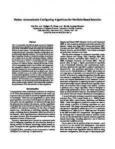
Number of Stocks Figure 2. Performance vs. Portfolio Size
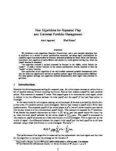
The improvement in the performance of ONS with increasing number of stocks is quite stark. The reason for this seems to be that ONS does an extremely good job of tracking the best stock in a given portfolio. Adding more stocks causes some good stock to get added, which ONS proceeds to track. Other algorithms behave more like the uniform CRP and so average out the increase in wealth due to the addition of a good stock. Figure 3 shows how ONS tracks CMC, which out-performs Kin-Ark for the test period, in a dataset composed of Kin-Ark and CMC (also used by Cover) while other algorithms have a nearly uniform distribution on both the stocks. This is the reason ONS outperforms all other algorithms on this dataset, as can be seen in Figure 5.
4.1. Performance vs. Portfolio Size
1
Since we implemented Cover’s algorithm by random sampling, there is a small degree of variability in the measurements recorded here. We used 1000 samples, which as suggested by (Stoltz & Lugosi, 2005), is sufficient to get a good estimate of the behavior of that algorithm. 2 The set of stocks used was RTN, SLB, ABK, PEG, KMG, FITB, CL, PSA, DOV, NKE, AT, NEM, VMC, D, CPWR, NVDA, SRE, HPQ, CMX, LXK, GPC, ABI, PGL, QLGC, OMX, QCOM, KO, PMTC, SWK, CTXS, FSH, HON, COF, LH, KMG, BLL, WB, OMX, K, LUV, DIS, SFA, APOL, HUM, CVH, IR, SPG, WY, TYC, NKE.
1 Fraction of CMC in portfolio
To measure the dependence of the performance of various algorithms on portfolio size we picked 50 sets of n random stocks from the data set, for values of n ranging from 5 to 40. All algorithms were run on the data, trading once every two weeks. The choice of trading period was to permit completion of the Universal al-
0.9 BCRP MW UCRP IR−MW ONS
0.8 0.7 0.6 0.5 0.4 0
1000
2000
3000 4000 Trading days
5000
Figure 3. How ONS tracks CMC.
6000
Newton Method based Portfolio Management
4.2. Random Stocks from S&P 500
30
25 UCRP Universal MW IR−MW ONS
20
UCRP Universal MW IR−MW ONS
25
20
APY
We tested the average APYs (over 50 trials of 10 random stocks from the S&P 500 list mentioned before) of the algorithms, for different frequencies of rebalancing, namely daily, weekly, fortnightly and monthly. As can be seen in figure 4 the performance of the ONS algorithm is superior to all other algorithms in all the 4 cases. As is expected the performance of all algorithms degrades as trading frequency decreases, but not very significantly. The simple strategy of maintaining a uniform constant-rebalanced portfolio seems to outperform all previous algorithms. This rather surprising fact has been observed by Borodin et al. (2004) also.
15
10
5
0
Iroq.&Kin−Ark CMC&Kin−Ark
25
0
daily
weekly fortnightly Trading frequency
monthly
Figure 4. Performance vs. Trading Period.
Wealth achieved per dollar
5
IBM&KO
Figure 5. Four pairs of stocks tested by Cover (1991) and Helmbold et al. (1998).
15
10
CMC&MEI
20
BCRP ONS IR−ONS
15
10
5
0 0
1000
2000
3000 4000 Trading days
5000
6000
4.3. Cover’s Experiments We replicated the experiments of Cover and Helmbold et al. on Iroquios Brands Ltd. and Kin Ark Corp., Commercial Metals (CMC) and Kin Ark, CMC and Meicco Corp., IBM and Coca Cola for the same 22 year period from 3rd July, 1962 to 31st December, 1984. As can be seen from Figure 5, ONS outperforms all other algorithms except on the Iroquios Brands Ltd. and Kin Ark Corp. dataset. Figure 6 shows how the total wealth (per dollar invested) varies over the entire period using the different algorithms for a portfolio of IBM and Coke. The ONS algorithm, and its internal regret variant IR-ONS, outperform even the best constant-rebalanced portfolio. 4.4. Stock Volatility We took the 50 stock data set used in previous experiments which had a history for 1000 days traded fortnightly and sorted them according to volatility and created two sets: the 10 stocks with largest and small-
Figure 6. Wealth achieved by various algorithms on a portfolio consisting of IBM and Coke.
est price variance. Then we applied the different algorithms on the two different sets. Figure 7 shows that the performance of ONS increases with market volatility whereas the performance of other algorithms decreases. 4.5. Margins Loans In line with Cover (1991) and Helmbold et al. (1998), we also tested the case where the portfolio can buy stocks on margin. The data set we tested on was the 22 year IBM and Coca Cola data mentioned earlier. Results for this case are given in Table 4. The margin purchases we incorporate are 50% down and 50% loan. The ONS algorithm in fact enhances its performance edge over other algorithms if margin loans are allowed.
Newton Method based Portfolio Management Table 2. Sharpe ratios for various algorithms on different datasets.
Iro.&Kin-Ark CMC & Kin-Ark CMC & Meicco IBM & Coke
Universal 0.4986 0.5740 0.3885 0.5246
UCRP 0.5497 0.6020 0.3834 0.5376
MW 0.5390 0.5980 0.3856 0.5356
IR-MW 0.5078 0.5812 0.3854 0.5295
ONS 0.4578 0.7466 0.5177 0.5824
Table 3. Minimum variance CRPs for various algorithms on different datasets. The number to the left of the slash is the volatility of the minimum variance CRP and the number to the right is the volatility of the algorithm on the dataset.
Iro. & Kin-Ark CMC & Meicco
Universal 0.4598/0.4948 0.1911/0.2728
UCRP 0.4929/0.4929 0.1909/0.2723
25 UCRP Universal MW IR−MW ONS
mean APY
20 15 10 5 0
low
high volatility
Figure 7. Performance of algorithms on high and low volatility datasets.
Table 4. Incorporating margin loans.
Algorithm UCRP Universal MW IR-MW ONS
APY, no margin 12.73 12.46 12.57 12.57 13.68
APY with margin 14.84 14.40 14.39 14.62 16.15
4.6. Sharpe Ratio and Mean-Variance Optimal CRPs It is a well-known fact that one can achieve higher returns by investing in riskier assets (Luenberger, 1998). So it is important to rule out the possibility of the ONS algorithm achieving higher returns compared to other algorithms by trading more riskily. Parameters like the Sharpe ratio and the optimal mean-variance portfolio are used to measure this risk versus reward tradeoff. R −R Sharpe ratio is defined as pσp f where Rp is the average yearly return of the algorithm, which indicates
MW 0.4803/0.4928 0.1909/0.2717
IR-MW 0.4606/0.4930 0.1909/0.2718
ONS 0.4603/0.5451 0.2070/0.3510
reward, Rf is the risk-free rate (typically the average rate of return of Treasury bills), and σp is the standard deviation of the returns of the algorithm, which indicates its volatility risk. Higher the Sharpe Ratio the better is the algorithm at balancing high rewards with low risk. The mean-variance optimal CRP for an algorithm is the CRP which achieves the same return as the algorithm but has minimum variance. This is the least risky CRP one could have used in hindsight to produce the same returns. The closer the volatility of the CRP to that of the algorithm, the better the algorithm is avoiding risk. Table 2 shows that ONS has either the best or slightly smaller Sharpe ratio among all algorithms. In Table 3, it can be seen that ONS has comparable volatility to the minimum variance CRP, implying that ONS does not take excessive risk in its portfolio selection. In the case of IBM & Coke and Kin-Ark & CMC, ONS beats the Best CRP in hindsight. Hence the concept of the optimal mean-variance CRP does not apply and the results for this case are omitted. 4.7. Running Times As expected, ONS runs slightly slower than MW, but both are much faster than Universal. We measured the running time (in seconds) of these algorithms on the 22 year data sets mentioned earlier. The machine used was a dual Intel 933MHz PIII processor with 1GB operated with Linux Fedora Core 3 operating system. The average running time, on the four data sets we considered, was 4882 seconds for the Universal algorithm3 , whereas MW and ONS took 3.7 and 26.7 seconds, respectively. This clearly shows the significant advantage of ONS over Universal and that it is comparable with MW in terms of computational efficiency. 3
With 1000 samples.
Newton Method based Portfolio Management
5. Conclusions We experimentally tested the recently proposed algorithms of (Agarwal & Hazan, 2005; Hazan et al., 2006) for the universal portfolio selection problem. The Online Newton Step algorithm is extremely fast in practice as expected from the theoretical guarantees. Moreover, it seems to be better than previous algorithms at tracking the best stock. It would be interesting to combine the anti-correlated heuristic of Borodin et al. (2004) with the best stock tracking ability of our algorithm. Another open problem is to incorporate transaction costs into the algorithm, as done by Blum and Kalai (1999) for Cover’s algorithm.
Acknowledgements We would like to thank Sanjeev Arora and Moses Charikar for helpful suggestions. Elad Hazan and Satyen Kale were supported by Sanjeev Arora’s NSF grants MSPA-MCS 0528414, CCF 0514993, ITR 0205594. We would also like to thank Gilles Stoltz for providing us with the data sets for experiments and helpful suggestions.
References Agarwal, A., & Hazan, E. (2005). New algorithms for repeated play and universal portfolio management. Princeton University Technical Report TR-740-05. Algoet, P., & Cover, T. (1988). Asymptotic optimality and asymptotic equipartition properties of logoptimum investment. Annals of Probability, 2, 876– 898. Bell, R., & Cover, T. (1980). Competitive optimality of logarithmic investment. Mathematics of Operations Research, 2, 161–166. Bell, R., & Cover, T. (1988). Game-theoretic optimal portfolios. Management Science, 6, 724–733. Blum, A., & Kalai, A. (1999). Universal portfolios with and without transaction costs. Machine Learning, 35, 193–205. Borodin, A., El-Yaniv, R., & Gogan, V. (2004). Can we learn to beat the best stock. Journal of Artificial Intelligence Research, 21, 579–594. Brookes, M. (2005). The matrix reference manual. [online] www.ee.ic.ac.uk/hp/staff/dmb/matrix/intro.html.
Cover, T. (1991). Universal portfolios. Mathematical Finance, 1, 1–19. Hannan, J. (1957). Approximation to bayes risk in repeated play. In M. Dresher, A. W. Tucker and P. Wolfe, editors, Contributions to the Theory of Games, III, 97–139. Hazan, E., Kalai, A., Kale, S., & Agarwal, A. (2006). Logarithmic regret algorithms for online convex optimization. To appear in the 19th Annual Conference on Learning Theory (COLT). Helmbold, D., Schapire, R., Singer, Y., & Warmuth., M. (1998). On-line portfolio selection using multiplicative updates. Mathematical Finance, 8, 325– 347. Kalai, A., & Vempala, S. (2003). Efficient algorithms for universal portfolios. Journal Machine Learning Research, 3, 423–440. Kalai, A., & Vempala, S. (2005). Efficient algorithms for on-line optimization. Journal of Computer and System Sciences, 71(3), 291–307. Kelly, J. (1956). A new interpretation of information rate. Bell Systems Technical Journal, 917–926. Larson, D. C. (1986). Growth optimal trading strategies. Ph.D. dissertation, Stanford Univ., Stanford, CA. Lov´asz, L., & Vempala, S. (2003a). The geometry of logconcave functions and an O∗ (n3 ) sampling algorithm (Technical Report MSR-TR-2003-04). Microsoft Research. Lov´asz, L., & Vempala, S. (2003b). Simulated annealing in convex bodies and an O∗ (n4 ) volume algorithm. Proceedings of the 44th Symposium on Foundations of Computer Science (FOCS) (pp. 650–659). Luenberger, D. G. (1998). Investment science. Oxford: Oxford University Press. Merhav, N., & Feder, M. (1992). Universal sequential learning and decision from individual data sequences. 5th COLT (pp. 413–427). Pittsburgh, Pennsylvania, United States. Ordentlich, E., & Cover, T. M. (1996). On-line portfolio selection. 9th COLT (pp. 310–313). Desenzano del Garda, Italy. Stoltz, G., & Lugosi, G. (2005). Internal regret in on-line portfolio selection. Machine Learning, 59, 125–159.