Algorithms for Provisioning Virtual Private Networks in the ... - CiteSeerX

Algorithms for Provisioning Virtual Private Networks in the Hose Model Amit Kumar
Rajeev Rastogi Avi Silberschatz Bulent Yener 600 Mountain Avenue Murray Hill, NJ 07974

Abstract Virtual Private Networks (VPNs) provide customers with predictable and secure network connections over a shared network. The recently proposed hose model for VPNs allows for greater flexibility since it permits traffic to and from a hose endpoint to be arbitrarily distributed to other endpoints. In this paper, we develop novel algorithms for provisioning VPNs in the hose model. We connect VPN endpoints using a tree structure and our algorithms attempt to optimize the total bandwidth reserved on edges of the VPN tree. We show that even for the simple scenario in which network links are assumed to have infinite capacity, the general problem of computing the optimal VPN tree is NP-hard. Fortunately, for the special case when the ingress and egress bandwidths for each VPN endpoint are equal, we can devise an algorithm for computing the optimal tree whose time complexity is O(mn), where m and n are the number of links and nodes in the network, respectively. We present a novel integer programming formulation for the general VPN tree computation problem (that is, when ingress and egress bandwidths of VPN endpoints are arbitrary) and develop an algorithm that is based on the primal-dual method. Finally, we extend our proposed algorithms for computing VPN trees to the case when network links have capacity constraints. We show that in the presence of link capacity constraints, computing the optimal VPN tree is NP-hard even when ingress and egress bandwidths of each endpoint are equal. Our experimental results with synthetic network graphs indicate that the VPN trees constructed by our proposed algorithms dramatically reduce bandwidth requirements (in many instances, by more than a factor of 2) compared to scenarios in which Steiner trees are employed to connect VPN endpoints.

1 Introduction Virtual Private Networks (VPNs) are becoming an increasingly important source of revenue for Internet Service Providers (ISPs). Informally, a VPN establishes connectivity between a set of geographically dispersed endpoints over a shared network infrastructure. The goal is to provide VPN endpoints with a service comparable to a private dedicated network established with leased lines. Thus, providers of VPN services need to address the QoS and security issues associated with deploying a VPN over a shared IP network. In recent years, substantial progress in the technologies for IP security [KA98, DGG + 98] have enabled existing VPN service offerings to provide customers with a level of privacy comparable to that offered by a dedicated line. However, ISPs have been slow to offer customers with guaranteed bandwidth VPN services since IP networks in the past had little support for enforcing QoS in the network. The recent emergence of IP technologies like MPLS and RSVP, however, have made it possible to realize IP-based VPNs that can provide end customers with QoS guarantees. In this paper, we address the problem of provisioning VPN services with QoS guarantees, a problem which has received little attention from the research community.
Current Address: Department of Computer Science, Cornell University.

0

1.1

The Hose Model

There are two popular models for providing QoS in the context of VPNs - the “pipe” model and the “hose” model [DGG+ 98, DR00]. In the pipe model, the VPN customer specifies QoS requirements between every pair of VPN endpoints. Thus, the pipe model requires the customer to know the complete traffic matrix; that is, the load between every pair of endpoints. However, the number of endpoints per VPN is constantly increasing and the communication patterns between endpoints are becoming increasingly complex. As a result, it is almost impossible to predict traffic characteristics between pairs of endpoints required by the pipe model. The hose model alleviates the above-mentioned shortcomings of the pipe model. In the hose model, the VPN customer specifies QoS requirements per VPN endpoint and not every pair of endpoints. Specifically, associated with each endpoint, is a pair of bandwidths – an ingress bandwidth and an egress bandwidth. The ingress bandwidth for an endpoint specifies the incoming traffic from all the other VPN endpoints into the endpoint, while the egress bandwidth is the amount of traffic the endpoint can send to the other VPN endpoints. Thus, in the hose model, the VPN service provider supplies the customer with certain guarantees for the traffic that each endpoint sends to and receives from other endpoints of the same VPN. The customer does not have to specify how this traffic is distributed among the other endpoints. As a result, in contrast to the pipe model, the hose model does not require a customer to know its traffic matrix, which in turn, places less burden on a customer that wants to use the VPN service. In summary, the hose model provides customers with the following advantages over the pipe model [DGG + 98]: 1. Ease of Specification. Only one ingress and egress bandwidth per hose endpoint needs to be specified, compared to bandwidth for each pipe between pairs of hose endpoints. 2. Flexibility. Traffic to and from a hose endpoint can be distributed arbitrarily over other endpoints as long as the ingress and egress bandwidths of each hose endpoint are not violated. 3. Multiplexing Gain. Due to statistical multiplexing gain, hose ingress and egress bandwidths can be less than the aggregate bandwidth required for a set of point to point pipes. 4. Characterization. Hose requirements are easier of characterize because the statistical variability in the individual source-destination traffic is smoothed by aggregation into hoses. The multiplexing gain due to the hose model (point 3 above) can result in significant improvements in the utilization of network resources. For example, consider a VPN used to offer VoIP service to customers located at VPN endpoints in NY, LA and Chicago. Suppose N is the maximum volume of calls out of NY (bounded by the number of customers being served by the VPN endpoint in NY). Further, suppose that there is a large variability in the destinations of the calls with as many as 80% of all calls out of NY being directed to LA at some times and to Chicago at other times. Thus, in the pipe model, two pipes, one from NY to LA and another from NY to Chicago, each with bandwidth to carry 0:8
N calls need to be reserved. As a result, in the pipe model, the total bandwidth reserved for traffic out of NY is 1:6
N units. In contrast, in the hose model, bandwidth is reserved only for the aggregate traffic out of NY, which is N units. Thus, by reserving bandwidth for the aggregate traffic out of VPN endpoints, the hose model improves network bandwidth utilization because of statistical multiplexing effects. From the above discussion, it follows that the hose model provides VPN customers with a simple mechanism for specifying bandwidth requirements and enables VPN service providers to utilize network bandwidth more efficiently. However, in order to realize these benefits, efficient algorithms must be devised for provisioning hoses. These hose provisioning algorithms need to set up paths between every pair of VPN endpoints such that the aggregate bandwidth reserved on the links traversed by the paths is minimum. A naive algorithm that sets up independent shortest paths between every pair of endpoints, however, could lead to excessive bandwidth being reserved. The reason for this is that the hose model provides the flexibility for traffic from a hose endpoint to be arbitrarily distributed to other endpoints. Consequently, the distribution of traffic between VPN endpoints is nondeterministic and the provisioning algorithms need to reserve sufficient bandwidth to accommodate the worst-case 1

1 (1) A

1 (1) B

A

1

1

1 (1) B 1

1

1 1 2

C

3 (2)

2 (2) (a) Graph

2

C

2

3 (2)

2 (2)

(b) Independent Shortest Paths

C

2

3 (2) 2 (2) (c) Link Sharing Among Paths

Figure 1: Link Sharing Among Paths to Reduce Reserved Bandwidth traffic distribution among endpoints that meets the ingress and egress bandwidth constraints of hose endpoints. Intuitively, in order to conserve bandwidth and realize the multiplexing benefits of the hose model, paths entering into and originating from each hose endpoint need to share as many links as possible. Thus, sophisticated hose provisioning algorithms need to be developed to ensure that the amount of bandwidth reserved in order to meet the hose traffic requirements is minimum. Example 1.1: Consider the network graph in Figure 1(a). The 3 VPN hose endpoints 1, 2 and 3 have bandwidth requirements of 1, 2 and 2 units, respectively (each endpoint has equal ingress and egress bandwidths). Figure 1(b) depicts the bandwidth reserved on relevant links of the network when a naive independent shortest paths approach is used to connect VPN endpoints. For instance, the shortest path between 1 and 2 passes through A, while the shortest path between endpoints 2 and 3 passes through C. Also, 1 unit of bandwidth needs to be reserved (in each direction) on the two links incident on A and on the shortest path from 1 to 2 since endpoint 1 can send/receive at most 1 unit of traffic. Similarly, the bandwidth reserved on the two links incident on C is 2 units, the minimum of the bandwidth requirements of endpoints 2 and 3. Thus, the total reserved bandwidth using independent shortest paths is 8 units (only considering one direction for each link). The reserved bandwidth can be reduced from 8 to 6 by exploiting link sharing among paths connecting the VPN endpoints as illustrated in Figure 1(c). Here, both paths from endpoint 1 to the two other endpoints pass through C, thus allowing the two links connecting 1 to C to be shared between them. (Note that the path from 1 to 2 passing through C is longer than the path from 1 to 2 through A). Further, since endpoint 1 cannot receive or send more than 1 unit of traffic, the bandwidth reserved on each of the two links is 1 unit (in each direction) and is shared between the two paths. Thus, the total bandwidth reserved decreases from 8 to 6 as a result of link sharing between paths. Note that provisioning pipes between each pair of VPN endpoints in the pipe model is somewhat simpler since the traffic between every pair of endpoints is fixed and is input to the provisioning algorithm. Thus, the VPN provisioning problem simply reduces to that of computing a set of fixed bandwidth paths between VPN endpoint pairs, which is an instance of the well-studied multicommodity flow problem [AMO93, Hoc97]. However, as mentioned earlier, the drawback of the pipe model is the difficulty of capturing and specifying bandwidth requirements between each pair of VPN endpoints. Thus, the hose model trades off provisioning simplicity for ease of specification and multiplexing gains.

2

1.2

Our Contributions

In this paper, we develop novel algorithms for provisioning VPNs in the hose model. In order to take advantage of the multiplexing gain possible due to hoses, we connect VPN endpoints using a tree structure (instead of independent point-to-point paths between VPN endpoints). A VPN tree has several benefits, which we list below. 1. Sharing of bandwidth reservation. A single bandwidth reservation on a link of the tree can be shared by the entire traffic between the two sets of VPN endpoints connected by the link. Thus, the bandwidth reserved on the link only needs to accommodate the aggregate traffic between the two sets of VPN endpoints. 2. Scalability. For a large number of VPN endpoints, a tree structure scales better than point-to-point paths between all VPN endpoint pairs. 3. Simplicity of Routing. The structural simplicity of trees ensures that if MPLS [DR00] is used for setting up paths between VPN endpoints, then fewer labels are required and label stacks on packets are not as deep. 4. Ease of Restoration. Trees also simplify restoration of paths in case of link failures, since all paths traversing a failed link can be restored as a single group, instead of each path being restored separately. We develop algorithms for computing optimal VPN trees; that is, trees for which the amount of total bandwidth reserved on edges of the tree is minimum. Initially, we assume that network links have infinite capacity, and show that even for this simple scenario, the general problem of computing the optimal VPN tree is NP-hard. However, for the special case when the ingress and egress bandwidths for each VPN endpoint are equal, we are able to devise a breadth first search algorithm for computing the optimal tree whose time complexity is O(mn), where m and n are the number of links and nodes in the network, respectively. We present a novel integer programming formulation for the general VPN tree computation problem (that is, when ingress and egress bandwidths of VPN endpoints are arbitrary) and develop an algorithm that is based on the primal-dual method [Hoc97]. Finally, we extend our proposed algorithms for computing VPN trees to the case when network links have capacity constraints. We show that in the presence of link capacity constraints, computing the optimal VPN tree is NP-hard even when ingress and egress bandwidths of each endpoint are equal. Further, we also show that computing an approximate solution that is within a constant factor of the optimum is as difficult as computing the optimal VPN tree itself. In [DGG+ 98], the authors suggest that a Steiner tree can be employed to connect VPN endpoints. However, our experimental results with synthetic network graphs indicate that the VPN trees constructed by our proposed algorithms require dramatically less bandwidth to be reserved (in many instances, by more than a factor of 2) compared to Steiner trees. Further, among the three algorithms, the primal-dual algorithm performs the best, reserving less bandwidth than both the breadth first search and Steiner tree algorithms over a wide range of parameter values.

2 System Model and Problem Formulation We model the network as a graph G = (V E ) where V is a set of nodes and E is a set of bidirectional links between the nodes. Each link (i j ) has associated capacities in the two directions – we denote the capacity from node i to j by Lij and the capacity (in the opposite direction) from node j to i by L ji . Also, Rij denotes the residual capacity (that is, the available bandwidth) of link (i j ) for carrying traffic from node i to j . In the hose model, each VPN specification consists of the following two components: (1) A set of nodes P  V corresponding to the VPN endpoints, and (2) For each node i 2 P , the hose ingress and egress bandwidths Biin and Biout , respectively. Without loss of generality, we assume that each node i 2 P is a leaf, that is, there is a single (bidirectional) link incident on i 1. As mentioned earlier, we consider tree structures to connect the VPN endpoints in P since trees are scalable, simplify routing and restoration. Further, trees allow the bandwidth In case there is a VPN endpoint i 2 P that is not a leaf, then we simply introduce a new node j in G and a new link (i
j ) with very large capacity, and replace node i in P with node j . 1

3

Symbol

G = (V
E ) m n L R i
j
l
u
v
w P T T B B T( ) P( ) C (i
j ) C d (i
j ) d (i
j ) ij

ij

v

in i out i i
j

i

i
j

i

T

T

T

G

Description Graph with nodes V and bidirectional edges E Number of links in graph G (jE j) Number of nodes in graph G (jV j) Capacity of link (i
j ) in the direction from node i to j Residual capacity of link (i
j ) in the direction from node i to j Generic symbols for nodes in G Set of VPN endpoints Generic notation for VPN tree VPN tree rooted at node v Ingress bandwidth for node i Egress bandwidth for node i Component of tree T containing i when link (i
j ) is deleted from T (i
j ) VPN endpoints contained in T i Bandwidth reserved on link (i
j ) of VPN tree T Sum of bandwidths reserved on all links of VPN tree T Distance (in number of links) between nodes i and j in tree T Length of the shortest path (in number of links) between nodes i and j in graph G

Table 1: Notation Used in the Paper reserved on a link to be shared by the traffic between the two sets of VPN endpoints connected by the link. Thus, the bandwidth reserved on a link must be equal to the maximum possible aggregate traffic between the two sets of endpoints connected by the link. Before we can compute the exact bandwidth to be reserved on each link of VPN tree T whose leaves are nodes (i
j ) (i
j ) the connected from P , we need to develop some notation. For a link (i j ) in tree T , we denote by Ti =Tj

( ) and P ( ) denote the set of

component of T containing node i=j when link (i j ) is deleted from T . Also, let P i

( )

( )

i
j

i
j

j

and Tj , respectively. Table 1 describes the notation used in the remainder of the paper. VPN endpoints in T i Observe that all traffic from one VPN endpoint to another traverses the unique path in the VPN tree T between (i
j ) and P (i
j ) . The the two endpoints. Now consider link (i j ) that connects the two sets of VPN endpoints P i j traffic from node i to j cannot exceed minf l2P ( ) Blout  l2P ( ) Blin g, that is, the minimum of the cumulai
j

i
j

P

P

i
j

i
j

( ) and the sum of ingress bandwidths of endpoints in P ( ) . This is tive egress bandwidths of endpoints in P ( ) and because the only traffic that traverses link (i j ) from i to j is the traffic originating from endpoints in P ( ) . The bound on the former is B , while the latter is bounded by directed towards endpoints in P i

j

i
j

i
j

i

j

P

i
j

P

2Pi(i
j)

l

T

in l

P

. Thus, the bandwidth to be reserved on link l

P

i
j

i

out l

l

i
j

P

j

(i j ) of T

out l

i to j is given by C B B g. Similarly, the bandwidth that must be reserved on link (j i) in 2 ( ) 2 ( ) P P the direction from j to i can be shown to be C (j i) = minf 2 ( ) B  2 ( ) B g. Note that C (i j ) may not be equal to C (j i). P Thus, the total bandwidth reserved for tree T is given by C = ( )2 C (i j ) (note that (i j ) and (j i) are considered as two distinct links in T ). Further, since we are interested in minimizing the reserved bandwidth for tree T , the problem of computing the optimal VPN tree becomes the following:

P (i j ) = minf

2Pj(i
j)

l

B

j

i
j

i

in the direction from

in l

T

l

i
j

P

i

in l

l

P

j

i
j

out l

T

T

T

i
j

T

T

Problem Statement (Optimal VPN Tree without Link Capacity Constraints): Given a set of VPN endpoints P , and their ingress and egress bandwidths, compute a VPN tree T whose leaves are nodes in P and for which CT is minimum.

4

0

1 (1000)

2 (1)

3 (1)

(a) Graph

0

4 (1)

5 (1)

6 (1000)

1 (1000)

2 (1)

3 (1)

4 (1)

5 (1)

6 (1000)

1 (1000)

(b) Steiner Tree

Figure 2: Example of Suboptimal Steiner Tree

5

2 (1)

3 (1)

4 (1)

5 (1)

(c) Optimal VPN Tree

6 (1000)

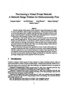
In [DGG+ 98], it has been suggested that a Steiner tree can be used to connect the VPN endpoints. However, even though a Steiner tree has the smallest number of links, it may be suboptimal, as illustrated by the following example. Example 2.1: Consider the network graph shown in Figure 2(a). Nodes 1 2 : : : 6 are the VPN endpoints and B1in = B1out = B6in = B6out = 1000 while Biin = Biout = 1 for i = 2 : : : 5. Figure 2(b) shows the Steiner tree connecting the VPN endpoints in P and containing 16 edges. The total bandwidth reserved on the edges of the Steiner tree (in a single direction) is given by 1000
2 + 1001
2 + 1002
2 + 1001
2 + 1000
2 = 10008 (this excludes the 2006 units that need to be reserved on the links incident on the VPN endpoints in P ). The reason for this is that 1000 units need to be reserved on the two links connecting endpoints 1 and 2, 1001 units need to be reserved on the two links connecting endpoints 2 and 3, and so on. However, the optimal VPN tree containing 17 links is shown in Figure 2(c). The cumulative bandwidth reserved on all the links of the optimal tree is 1000
2+1000
2+4+2
2+1
2+1
2 = 4012 (again, in a single direction per link and excluding the 2006 units that need to be reserved on the links incident on the VPN endpoints in P ). This is because the bandwidth reserved on the two links connecting endpoints 1 and 0 is 1000, the bandwidth for the two links between endpoints 6 and 0 is 1000, the bandwidth for the link connecting 0 to endpoints 2 : : : 5 is 4 units, and for the two links connecting endpoints 3 and 4 is 2 units, and so on. Thus, in the above example, the bandwidth reserved for the Steiner tree is more than twice the optimum bandwidth. Further, note that, in the example, the performance of the Steiner tree can be made arbitrarily worse compared to the optimum (by increasing the number of VPN endpoints between endpoints 1 and 6). In our earlier formulation of the optimal VPN tree computation problem, we assumed that links do not have capacity constraints. In the following, we present the problem formulation that also takes into account the residual bandwidths of network links. Problem Statement (Optimal VPN Tree with Link Capacity Constraints): Given a set of VPN endpoints P , and their ingress and egress bandwidths, compute a tree T whose leaves are nodes in P such that C T (i j )  Rij and CT is minimum. In the remainder of the paper, we will refer to CT (i j ) as the cost of link (i j ) in tree T and C T as the cost of tree T . In the following two sections (Sections 3 and 4), we first develop algorithms to compute the optimal VPN tree ignoring link capacity constraints. We then show how the algorithms can be extended to handle link capacity constraints in Section 5.

3 Symmetric Ingress and Egress Bandwidths For symmetric ingress and egress bandwidths, that is, when B iin = Biout for each VPN endpoint i, one can devise efficient algorithms for computing the minimum cost VPN tree if links do not have capacity constraints. In this section, we present a polynomial time algorithm for computing the optimal VPN tree for the symmetric bandwidth case under the assumption that the residual capacity of each edge is large. Since the ingress and egress bandwidths are equal, in the following, we simply drop the superscripts in and out, and denote the bandwidth for endpoint i simply by Bi . Before presenting our algorithm for computing the optimal tree (that is, tree with minimum cost), we first develop some intuition for the cost C T of a tree T . Recall (from the previous section) that CT = (i
j )2T CT (i j ).

P

( )

P

( )

For a set of leaves L  P , we define B (L) as l2L Bl . Thus, CT (i j ) = minfB (Pi ) B (Pj )g. It is straightforward to observe that C T (i j ) = CT (j i), that is, the bandwidth reserved on link (i j ) in the two directions is equal. Now suppose that for a tree T and a node v in T , we define the quantity Q(T v ) to be 2
l2P Bl
dT (v l), where the sum is over all leaves l, and dT (v l) denotes the length of the unique v to l path in T . Then, for any tree T whose leaves are nodes in P , we can show that CT satisfies the following two properties: i
j

P

6

i
j

 Property 1. There exists a node w 2 T such that CT  Property 2. For all nodes v 2 T , CT  Q(T v ). In order to show the above two properties for tree direction to each edge e = (i j ) of T as follows:

= Q(T w).

T , we construct a directed tree T

dir

T

from

by giving a

( ) ) < B (P ( ) ), then direct the edge towards i. ( ) ) < B (P ( ) ), then direct the edge towards j .  if B (P ( ) ) = B (P ( ) ), then direct the edge towards the component which contains a particular leaf, say,  if B (P  if B (Pi

i
j

i
j

j

i
j

i
j

j

i

i
j

i
j

i

^l.

j

Clearly, Tdir must contain a node whose indegree is 0 — we denote this node in T dir with no incoming edges by a(T ). We show that a(T ) is indeed unique and C T = Q(T a(T )). For this, we prove some properties about Tdir in the following lemma. Lemma 3.1: Every edge e in Tdir is directed away from a(T ). Proof: Let e = (i j ) be an edge in tree T such that i is closer to a(T ) than j in T . We show that e is directed from i to j in Tdir . Consider the path in T from a(T ) to i. We know that the first edge (u v ) along the path is (u
v) (u
v) directed away from u = a(T ). So, B (Pv )  B (Pu ). Since (u v ) is the first edge of the path from a(T ) (u
v)  P (i
j ) and also, P (i
j )  P (u
v) . Thus, we get, B (P (i
j ) )  B (P (u
v) )  B (P (u
v) )  B (P (i
j ) ). to i, Pu v v u i j j i

B (P ( ) ) < B (P ( )), then edge e is directed from i to j and we are done. The only other possibility is B (P ( ) ) = B (P ( )). But then, it must be the case that P ( ) = P ( ) , P ( ) = P ( ) and B(P ( ) ) = B(P ( ) ). As a result, it follows that u = i and v = j , and since edge (u v) is directed from u to v , edge (i j ) must also be directed from i to j . Note that from the above lemma, one can easily show that a(T ) is unique since every other node in T has i
j

If

i
j

j

i

i
j

i
j

j

u
v u

i

i
j

u
v

i
j

v

i

u
v

u

j

u
v

v

dir

an edge directed into it (and consequently, an indegree of 1). In the following lemma, we prove that Property 1 mentioned above holds for w = a(T ). Lemma 3.2: The cost of tree T , CT

= Q(T a(T )). Proof: Let l be a leaf and e = (i j ) be an edge on the path from a(T ) to l (node i being closer to a(T )) — ( ) ) since due note that B contributes to both C (i j ) and C (j i). The reason for this is that C (i j ) is B (P ( ) )  B (P ( ) ). Thus, since l 2 P ( ) , B to Lemma 3.1, the edge is directed from i to j in T and so B (P contributes to each edge on the path from a(T ) to l, and to no other edge. This proves the lemma. Property 2 is a straightforward corollary of the following lemma (since C = Q(T a(T )) due to Lemma 3.2). Lemma 3.3: Let v be any node in T . Then, Q(T a(T ))  Q(T v ). Proof: We first show the following result: suppose e = (i j ) is an edge that is directed from i to j in T . Then, Q(T i)  Q(T j ). We know that B (P ( ))  B(P ( )). Now, i
j

l

T

T

T

i
j

dir

j

i
j

j

i
j

i

j

T

dir

i
j

X

i
j

j

Q(T i) ; Q(T j ) = 2
l

=

B
(d (i l) ; d (j l)) + 2
l

(i
j )

X

T

T

X

2Pi

;2
l

(i
j )

2Pi

B +2
l

l

(i
j )

B

l

2Pj

i
j

i
j

i

7

(i
j )

2Pj

l

= 2
B (P ( ) ) ; 2
B (P ( ) ) j

X

i



0

B
(d (i l) ; d (j l)) l

T

T

l

procedure C OMPUTE T REE S YMMETRIC(G, P ) 1. Topt :=
2. for each node v in G f 3. Tv := v 4. openQ := fvg 5. while (openQ = 6
)f 6. dequeue first node u from openQ 7. for each edge (u
w) in G such that w is not in Tv f 8. add edge (u
w) to Tv 9. append node w to end of openQ 10. g 11. prune leaves of Tv that do not correspond to VPN endpoints (that is, do not belong to P ) 12. if CTv < CTopt 13. Topt := Tv 14. g 15. return Topt

Figure 3: Algorithm for Computing Optimal Tree for Symmetric Bandwidths Now, we can prove the lemma. Consider the path from a(T ) to v in Tdir . By Lemma 3.1, all edges along the path are directed away from a(T ). So, repeated application of the result proved above (for each edge along the path) proves the lemma. From Properties 1 and 2, it follows that for the optimal tree T opt, CT = Q(Topt a(Topt)). Thus, if we could compute, for each node v , the tree Tv such that Q(Tv  v ) is minimum, then the optimal tree is simply the tree Tv with the minimum Q(Tv  v). Figure 3 contains the procedure for computing the optimal tree Topt. For each node v in G, Procedure C OMPUTE T REE S YMMETRIC computes a breadth first spanning tree rooted at v — we show in Lemma 3.4 below that this tree T v minimizes the value of Q(Tv  v ) among possible trees rooted at v . The procedure then outputs the tree T v for which Q(Tv  v ) is minimum — let Tv^ be this tree. In the following, we show that C T^ = CT where Topt is the optimal tree. First note the following important fact for the breadth first tree Tv rooted at node v . opt

v

opt

Lemma 3.4: Let T be any tree and v be a node in G. Then, Q(Tv  v )  Q(T v ). Proof: Note that dT

v

(v l)  d (v l) for each leaf l in T . So, the lemma is true. T

In the next lemma, we show the following important relationship between T v^ and Topt that enables us to subsequently show that their costs are equal. Note that due to Lemma 3.2, C T = Q(Topt a(Topt)). opt

Q(T^ v^)  Q(T  a(T )) = C : Proof: Lemma 3.4 above implies that Q(T ( )  a(T ))  Q(T  a(T )). Since Q(T^ v^) is minimum among all nodes v in the graph, Q(T ^ v^)  Q(T ( )  a(T )) and the lemma follows. Lemma 3.5:

v

opt

opt

Topt

a Topt

v

Theorem 3.6:

C ^=C Tv

Topt

a Topt

opt

opt

opt

v

opt

:

Proof: First, due to Lemma 3.2, CT^ = Q(Tv^ a(Tv^)). Further, Lemma 3.3 implies that Q(Tv^ a(Tv^))  Q(Tv^ v^), which by Lemma 3.5 is at most CT . Thus, it must be the case that CT^ is optimum. v

opt

v

It is straightforward to observe that the time complexity of Procedure C OMPUTE T REE S YMMETRIC is O(mn), where n = jV j is the number of nodes and m = jE j is the number of edges in G. This is because the outermost for loop iterates over every node in G, and the body of the for loop, in the worst case, considers every edge in G. 8

(3/6) 0

7

5

3 3

9

3 8

6

6

4

6 6

(3/6) 1

3 (3/4)

3

6

4

4 (3/4)

2 (3/4)

Figure 4: Example of Tree Cost for Asymmetric Bandwidths

4 Asymmetric Ingress and Egress Bandwidths In this section, we address the case when VPN endpoint bandwidth requirements are asymmetric, that is, for a VPN endpoint j , Bjin and Bjout may be unequal. Asymmetric ingress and egress bandwidths complicate the VPN tree computation problem since for a VPN tree T connecting the VPN endpoints, the bandwidth reserved along edge (i j ) of T may not be identical in the two directions – that is, C T (i j ) may not be equal to CT (j i). This is because for an edge (i j ), CT (i j ) = minf l2P ( ) Blout  l2P ( ) Blin g and CT (j i) = minf l2P ( ) Blin  l2P ( ) Blout g.

P

P

i
j

i

P

i
j

P

i
j

j

i

i
j

j

Thus, in the asymmetric case, since Blin and Blout may not be equal, CT (i j ) and CT (j i) may not be equal. Note that this is different from the symmetric bandwidths case in which the bandwidths reserved in both directions along an edge (i j ) of a tree T were equal.

Example 4.1: Consider the VPN tree shown in Figure 4 connecting the VPN endpoints in P = f0 1 : : : 4g. The bandwidth requirements for the endpoints are as follows: for endpoints 0 and 1, B in = 3 and B out = 6, and for endpoints 2, 3 and 4, B in = 3 and B out = 4. The bandwidths reserved in the two directions for the various edges of the tree are shown adjacent to the edges in the figure. Thus, for instance, for edge (5 6), CT (5 6) = 9 (since out = 12 is greater than l2P (5 6) Blin = 9) and CT (6 5) = 6 (since l2P (5 6) Blout = 12 is greater (5 6) Bl l2P

P

P than

P

P

B = 6). Similarly, one can show that for edge (6 7), C (6 7) = 6 (since P 2 6(6 7) B = 16 is P P P greater than 2 (6 7) B = 6) and C (7 6) = 8 (since 2 (6 7) B = 8 is less than 2 (6 7) B = 9). 7 7 6 5




in l

(5
6)

2P5

l

6

l

P




6




T




in l

T

l

P




out l

l

l

P

P







out l

in l

For the asymmetric bandwidths case, the problem of computing the VPN tree with the minimum cost can be shown to be at least as difficult as that of computing a Steiner tree connecting the VPN endpoints. Since the Steiner tree computation problem for a set of VPN endpoints is NP-hard [Hoc97, GJ79], it follows that the problem of computing the optimal VPN tree is also NP-hard. Theorem 4.2: For the asymmetric bandwidths case, the problem of computing the optimal VPN tree connecting the set of VPN endpoints in P is NP-hard.

4.1

Integer Programming Formulation

In this section, we show that the problem of computing the optimal tree can be formulated as an integer programming problem. For this, we first need to examine the properties of VPN trees connecting endpoints with asymmetric bandwidths. For an edge (i j ) of VPN tree T , we say that it is biased towards i if the following two conditions hold:

9

P

1. (

^l), and

P

2. (

^l).

(i
j )

2Pi

l

(i
j )

2Pi

l

B 0g the set of eligible nodes for endpoint j . x y^ z^) that is Procedure C OMPUTE T REE ROUNDING shown in Figure 5 computes a feasible integer solution (^ x y z). The procedure begins by clustering the VPN endpoints within a constant factor of the fractional solution ( in Steps 6–16. Each cluster has a VPN endpoint j that is the seed of the cluster. The set of seed endpoints are stored in seedSet and Sj is the cluster with endpoint j as the seed. Every endpoint l 2 S j has the following properties: (1) j  l , (2) for some node i 2 Fl , dG (i j )  c0 j or for some node i 2 Fj , dG (i l)  c0l (here c0 > 1 is a constant that we define later). We will assign each endpoint in S j to some node in Fj , and the following lemma states that this will not increase the overall cost by much. Lemma 4.10: For each l 2 Sj and i 2 Fj , dG (i l)  (c0 + 2)
l . Proof: Consider an i 2 Fj . Due to the definition of F j , it follows that d G (i j )  two cases, one of which must hold because l 2 Sj .

13

 . We consider the following j

1. For some node i0 2 Fl , dG (i0 j )  c0j . Since i0 2 Fl , it must be the case that dG (i0 l)  l . Thus, due to the triangle inequality, d G (i l)  dG (i j ) + dG (i0 j ) + dG (i0 l) = (c0 + 1)j + l . Since j  l , the lemma follows. 2. For some node i0 2 Fj , dG (i0 l)  c0l . Since i0 2 Fj , it must be the case that dG (i0 j )  j . Thus, due to the triangle inequality, d G (i l)  dG (i j ) + dG(i0 j ) + dG(i0 l) = c0l + 2
j . Since j  l , the lemma holds. In order to maintain feasibility of the solution once endpoints in S j are assigned to some node in Fj , we need to construct a Steiner tree T that connects v to at least one node from F j for each j belonging to seedSet. To accomplish this, in the graph G, for each endpoint j in seedSet, we contract the nodes in each F j to a new supernode. We then connect the supernodes by a Steiner tree T , thus ensuring that each supernode is connected to v (Step 18). However, note that although T connects the supernodes (and v) in G 0, it may happen that T does not form a single connected subgraph in G. The reason for this is that edges of T may be incident on different nodes in an Fj . Thus, in order to ensure that T forms a connected subgraph even in G, in Steps 22–24, we select a node u in Fj and connect it to every other node of Fj on which an edge of T is incident. In the following lemma, we show that the number of edges in T v is within a constant factor of e2E ze . 0 Lemma 4.11: The number of edges in Tv is less than or equal to 2(cc0 ;+1) 1


P2 e

E

P

z . e

Proof: We first show that the number of edges in the Steiner tree T that connects the supernodes in G 0 = (V 0  E 0) is at most 2 e ze . Consider any set S V 0 containing a proper subset of the set of supernodes. Without loss of generality, we assume that S does not contain v (if S contains v , then we replace S by V 0 ; S ). Let S contain the supernode corresponding to endpoint j (resulting due to collapsing nodes in F j ). Since ( x y z) is a feasible ij  i2F xij = 1. So, if we consider an instance of the Steiner tree solution for LP (2), e2(S ) ze  i2S x problem with the set of supernodes as the set of nodes to be connected in G 0 , then ze is a feasible fractional solution to this problem. Thus, it is possible to construct a Steiner tree T connecting the supernodes containing at most 2 e ze edges [Hoc97]. We next show that for every j in seedSet, connecting node u 2 F j to every other node w in Fj with an outgoing 0 arc in Tdir (in Steps 22-24) increases the number of edges in T by a factor of at most cc0 +1 ;1 . First, observe that the length of the shortest path between u and w is at most 2
 j (since endpoint j is at a distance of at most  j from both u and w). Also, in T , there must be a path from w to a node i belonging to F l for some other l = 6 j in seedSet. Furthermore, dG (i j ) > c0j , since otherwise j and l would belong to the same cluster. Thus, the length of the path from w to i is at least (c0 ; 1)j . We charge the cost of 2j of connecting u to w to this segment of T – it is easy to show that disjoint segments of T will be charged in this manner. So, the number of edges in T increases by a factor of at most (c0 + 1)=(c0 ; 1). This proves the lemma.

P

P

P

P

j

P

We are now in a position to show the near-optimality of the final rounded integer solution (^ x y^ z^). In this solution, in addition to setting y^v = 1, for every j in seedSet, for node u 2 Fj that has an incoming arc in Tdir , y^u is set to 1, otherwise y^u is set to 0. Further, for every endpoint l 2 Sj , l is assigned to node u 2 Fj with the incoming arc, that is, x ^ul = 1. Finally, for every edge e in Tv , z^e = 1 and z^e = 0 for all other edges. The integer solution is clearly feasible since T v connects every u 2 Fj (that has an incoming arc in Tdir ) to v . Theorem 4.12: The cost of integer solution (^ x y^ z^) is within a factor of 10 of the cost of the optimal LP solution (x y z ).

P2

2P

d (i j )
B
x^ + M
P 2 Pz^ . Due to B
 . Also, due to Lemma 4.11, M
2 z^  z . Combining this with Equation (3) and since z  z =c, we get that the cost of (^x y^ z^) is j

j

Proof: The cost of the integer solution (^ x y^ z^) is given by Lemma 4.10, i2V
j 2P dG (i j )
Bj
x ^ij  (c0 + 2) j 2P

P M
2( +1) P 0

c

c0

;1

2E

e

P

e

i

V
j

G

ij

e

E

e

e

e

14

j

e

E

e

P

P

+2 dG(i j )
Bj
xij + 2(c(cc0 ;+1)1) M
e2E ze . Thus, (^x y^ z^) is within a constant factor of at most c1; i2V
j 2P c 0 +2 2(c0 +1)  c(c0 ;1) g. Choosing c = 53 and the optimal fractional solution (to the LP). This constant turns out to be maxf c1; c c0 = 2, we get a value of 10 for the constant. 0

0

Time Complexity. The time complexity of Procedure C OMPUTE T REE ROUNDING can be shown to be O(n2 (log n+ p)), where p = jP j and n = jV j. The first term n2 log n is the time complexity of constructing a Steiner tree in Step 18 [Hoc97], while the second term n2 p is due to the overhead of computing shortest paths for at most p (u w) node pairs in Steps 21–25.

4.3

Primal-Dual Algorithm

While the rounding based algorithm gives a constant factor performance guarantee on the cost of the computed VPN tree (with respect to the cost of the optimal tree), it requires solving the LP relaxation of the integer program. This LP relaxation has a small number of variables, but an exponential number of constraints. Even though the ellipsoid method can be used to solve the LP in polynomial time [Que93], it may not be computationally efficient and thus impractical. In this section, we propose an algorithm that employs the primal-dual method in order to find a feasible solution to the integer program (1). The dual for the LP relaxation (2) is as follows.

X

maximize

8i 2 V j 2 P

: 

j

;

8e 2 E

:

^

^

V

2P

X V

2V^
v62V^

X

V
i

V
e

8j 2 P

(4)

j

j

2(V^ )
v62V^

: 

j

^

 Bj
dG (i j )

^

M

Vj

Vj

0

8j 2 P V V^  v 62 V^

: ^

Vj

0

The dual is employed to guide in the selection of the set F j of potential nodes for each VPN endpoint j . The primal complementary slackness conditions imply the following:

 If endpoint j is assigned to node i 2 V , then  j ;

P  If edge e is a Steiner tree edge, then

P

2V^
v62V^

i

^ = B
d (i j ). j

Vj

G

^ = M. P ^ ^ ^ = B
d (i j ), while edges e for which of all nodes i for which  ; 2 62 PThus, ^F consists 2 ( ) 62 ^ ^ = M constitute potential Steiner tree edges. Once F for each endpoint j has been computed, Procedure C OMPUTE T REE ROUNDING (see Figure 5) is used to compute the final set of nodes S to which VPN j

e

 V


v

e

2(V^ )
v62V^ j

V

i

Vj

V
v

V

j

Vj

G

j

Vj

endpoints are to be assigned, and the Steiner tree connecting the nodes. The overall procedure for computing the optimal VPN tree is shown in Figure 6. Procedure C OMPUTE T REE PRIMAL D UAL uses the primal-dual method to compute a set of nodes S containing a specific node v 2 V and the Steiner tree edges connecting the nodes in S . This is done in the body of the for loop spanning Steps 2–38 for each node v 2 V and the tree with the smallest cost is returned. The primal-dual algorithm is an iterative algorithm – during each iteration, j for the VPN endpoint j with the smallest  j is increased and in order to preserve dual feasibility, the V^ j s are appropriately adjusted. When j for a VPN endpoint j becomes equal to dG (i j )
Bj for a node i 2 V , node i becomes a potential node for assigning endpoint j and is added to F j . Further, when for an edge e, the sum of V^ j s (for which e 2  (V^ )) becomes equal to M , the edge is added to the set of potential Steiner tree edges connecting the nodes that are chosen for VPN endpoints. The  j for a VPN endpoint j is not increased once one of the potential nodes for it (in F j ) becomes connected to v via potential Steiner tree edges. 15

This is because, as explained below, when  j is increased, dual feasibility cannot be maintained by increasing V^ j ,

where v 62 V^ .

Data Structures. The algorithm collects the potential nodes for a VPN endpoint j in F j . These are the nodes i for which j  Bj
dG (i j ). Also, for each edge e, we stores the sum of all the V^ j s that contribute to e – here

does not contain v and e 2  ( V^ ). Thus, when we = M , e becomes a potential Steiner tree edge. Also note that for any potential Steiner tree edge e, if e 2  (V^ ), then V^ j cannot be increased since this would result in a violation of dual feasibility. In the procedure, C u is used to store the nodes connected to u via potential Steiner tree edges. Finally, Sj is used to store the set of all nodes connected to nodes in F j via potential Steiner tree edges (thus Fj  Sj ). As mentioned earlier, once Sj contains v , then j for endpoint j cannot be increased any further.

V^

Algorithm. The complete primal-dual algorithm for computing the VPN tree with low cost is illustrated in Figure 6. For each v 2 V (in the outermost for loop), the algorithm first employs the primal-dual method to compute a set of potential nodes F j for each VPN endpoint j and a set of potential Steiner tree edges that connect each Fj to v (Steps 3–30). It then invokes Procedure C OMPUTE T REE ROUNDING to compute the Steiner tree containing v and connecting the nodes to which VPN endpoints are assigned. This tree is then extended to connect the VPN endpoints in P in Steps 32–35. The variable activeSet stores the VPN endpoints j for which  j can still be incremented. The set Sj denotes the smallest set V^ of nodes for which V^ j needs to be increased when j for a VPN endpoint j is increased. The reason for this is that for every i 2 F j , j  Bj
dG (i j ). Thus, in order to ensure that the dual equation j ; i2V^
v62V^ V^ j  Bj
dG(i j ) stays feasible when j is incremented, V^ j where i 2 V^ must also be

P

incremented. Note also that V^ j can be incremented only if  (V^ ) contains no potential Steiner tree edges. This is

P

because for a potential Steiner tree edge e, e2(V^ )
v62V^ V^ j = M . As a result, increasing V^ j if e 2  (V^ ) could cause the dual equation e2(V^ )
v62V^ V^ j  M to be violated. Thus, if V^ j is the variable that is increased to

P

maintain dual feasibility when  j for a VPN endpoint j is increased, then V^ must contain all the nodes in C i for every i 2 Fj , or alternately Sj  V^ . From the above discussion, it follows that if S j for a VPN endpoint j contains v , then  j cannot be increased any further. This is because there are no V^ j variables for sets V^ that contain node v . As a result, it is not possible to increase V^ j to ensure that the dual equation  j ; i2V^
v62V^ V^ j  Bj
dG (i j ) stays feasible when j is incremented. Thus, activeSet only contains VPN endpoints j for whom S j does not contain v . In each iteration of the while loop spanning Steps 7–30,  j for a single VPN endpoint j belonging to activeSet is incremented by minf 1  2g, where j , 1 and 2 are as defined in Steps 8–12. Note that increasing j causes one of the following to happen – (1) k to be added to F j since j = dG (j k) (if 1  2 ), or (2) edge e to become a potential Steiner tree edge since M = we (if 2 < 1 ). For the latter case, the connected components for nodes connected to u and v need to be adjusted (Steps 23 and 24). In addition, S j s for VPN endpoints j that contain either u or v need to be expanded as described in Steps 26 and 27. Finally, note that in order to maintain feasibility of equations  j ; i2V^
v62V^ V^ j  Bj
dG (i j ) for endpoints i in Fj , S j is increased by 1 = 2 when j is increased by 1 = 2 . This, in turn, contributes 1= 2 to we0 for all edges e0 2  (Sj ) (Steps 15 and 22).

P

P

j

Time Complexity. The time complexity of Procedure C OMPUTE T REE P RIMAL D UAL can be shown to be O(n(m2p+ mnp + n2 log n)), where p = jP j, m = jE j and n = jV j. The outermost for loop performs n iterations, one for each node v 2 V . Further, for each iteration of the outermost loop, the body of the if condition (Steps 14–18) can be executed at most np times, once for each VPN endpoint node pair, while the body of the else condition (Steps 21–28) can be executed at most m times, once for each edge in E . Assuming that unions involving S j can be performed in O(n) steps and lookups of S j can be carried out in constant time, the complexity of Steps 14-18 can be shown to be O(m + n), while the complexity of Steps 21–28 can be shown to be O(mp + np). Finally,

16

procedure C OMPUTE T REE P RIMAL D UAL(G, P ) 1. T :=
2. for each v 2 V f 3. for each i 2 V , Ci := fig 4. for each e 2 E , we := 0 5. for each j 2 P , Fj := fj g, Sj := fj g
j := 0 6. activeSet := P 7. while activeSet = 6
f 8. select a VPN endpoint j with minimum j =Bj from activeSet 9. let k be the node in V ; Fj such that dG(k
j ) is minimum 10. let e = (u
w) 2  (Sj ) such that M ; we is minimum 11. let 1 := dG(k
j )  Bj ; j 12. let 2 := M ; we 13. if 1  2 f 14. j := j + 1 15. for each e0 2  (Sj ), we0 := we0 + 1 16. Fj := Fj  fkg 17. Sj := Sj  Ck 18. if v 2 Sj , delete j from activeSet 19. g 20. elsef 21. j := j + 2 22. for each e0 2  (Sj ), we0 := we0 + 2 23. for each l 2 Cu, Cl := Cl  Cw 24. for each l 2 Cw , Cl := Cl  Cu 25. for each l 2 P f 26. if w 2 Sl , Sl := Sl  Cu 27. if u 2 Sl , Sl := Sl  Cw 28. if v 2 Sl , delete l from activeSet 29. g 30. g 31. g 32. Tv := computeTreeRounding(F
=B
G
P
v) 33. let G0 be the graph obtained from G as a result of coalescing all nodes in Tv into a supernode v 0 34. construct breadth first tree T 0 rooted at v 0 and whose leaves are the VPN endpoints in P 35. add edges in T 0 to Tv 36. delete leaves from Tv that do not correspond to VPN endpoints 37. if CTv < CT , T := Tv 38. g 39. return T

Figure 6: Primal-Dual Algorithm for Computing VPN Tree

17

as shown earlier, the time complexity of Procedure C OMPUTE T REE ROUNDING is O(n2 log n + n2 p). Thus, the Procedure C OMPUTE T REE P RIMAL D UAL has an overall time complexity of O(n(m2p + mnp + n2 log n)).

4.4

Breadth First Search Based Algorithm

The breadth first search algorithm presented in Section 3 can also be used to compute the VPN tree for the asymmetric bandwidth case (see Procedure C OMPUTE T REE S YMMETRIC in Figure 3). However, since the VPN tree computation problem for the asymmetric case is NP-hard, the algorithm may not return the optimal VPN tree. Nevertheless, one can show that cost of the tree computed by the procedure is within a factor of the cost of the optimal VPN tree.

P

P

2P

l

in l

B

+

B

M

out l

of

Theorem 4.13: The cost of the tree returned by Procedure C OMPUTE T REE S YMMETRIC is within a factor of 2P

l

in l

B

M

+

out l

B

of the cost of the optimal VPN tree.

Proof: Let Bj = Bjin + Bjout for VPN endpoint j . Consider the optimal tree Topt and let b = jbal(Topt)j be the number of balanced edges in Topt. Also let corej denote the core node closest to VPN endpoint j in T opt. Thus, the cost of Topt is at least j 2P dT (corej  j )
Bj + b
M . Now consider the breadth first tree Tv rooted at v , a core node, and computed by Procedure C OMPUTE T REE S YMMETRIC . The quantity j 2P dT (v j )
Bj is an upper bound on the cost of the tree T v (since the bandwidth reserved on an edge (u w) (w is further from v than u in T v ) is at most l2P ( ) Bl , each VPN endpoint j can contribute at most B j to the reserved bandwidth on edges along the path from v to j ). Now dT (v j )  b +dT (corej  j ). As a result, the cost of Tv is no more than j2P dT (corej  j )
Bj + j 2P b
Bj .

P

v

opt

P

P

v

opt

Thus, the ratio of the costs of trees T v and Topt is less than or equal to

b

P P


j




opt

2P

b M

Bj

u
w w

P

, which proves the lemma.

5 Incorporating Link Capacity Constraints The algorithms for computing VPN trees in the previous two sections do not take into account link capacity constraints, that is, the algorithms assume that each link has a large available bandwidth. In this section, we consider the problem of provisioning VPN trees when edges of the graph G have associated capacity constraints. Recall that Rij denotes the residual capacity of edge (i j ) - thus, R ij is the available bandwidth on link (i j ). We say that a VPN tree T is feasible if for each edge (i j ) in T , CT (i j )  Rij . In this section, we develop algorithms for computing a feasible VPN tree T with the minimum possible cost. In the presence of edge capacity constraints, the problem of computing the optimal VPN tree is NP-hard even when endpoints have equal ingress and egress bandwidths. Further, one can show that unless P = NP , it is impossible to approximate the optimal VPN tree to within a constant factor in polynomial time. Theorem 5.1: In the presence of edge capacity constraints, the problem of determining if there exists a feasible VPN tree T is NP-hard. Corollary 5.2: In the presence of edge capacity constraints, the problem of determining if there exists a feasible VPN tree whose cost is within a constant factor c of the optimal cost is NP-hard.

5.1

Symmetric Ingress and Egress Bandwidths

In Section 3, we showed that in the absence of link capacity constraints and when VPN endpoints had symmetric ingress and egress bandwidth requirements, considering the breadth first tree rooted at each node v 2 V , yielded the optimal VPN tree (see Procedure C OMPUTE T REE S YMMETRIC in Figure 3). In this subsection, we show how the procedure can be extended to handle link bandwidth constraints. 18

procedure C OMPUTE T REE S YMMETRIC C ONST(G, P , v) 1. Tv :=
2. S := P 3. make copy Gv of G (including residual capacities of edges in G) 4. while (S = 6
) f 5. T := v 6. openQ := fvg 7. while (openQ = 6
)f 8. dequeue first node u from openQ 9. for each edge (u
w) in Gv such that w is not in T f 10. if w is not in T v or edge (u
w) is in Tv 11. add edge (u
w) to T 12. append node w to end of openQ 13. g 14. g 15. prune leaves from T that do not correspond to remaining VPN endpoints (that is, do not belong to S ) 16. if T does not contain all the VPN endpoints in S 17. return
/* tree rooted at v cannot satisfy capacity constraints */ 18. compute maximum bandwidth MT
v (i
j ) to be reserved on each edge (i
j ) of the tree T rooted at v 19. violatedSet :=
20. while there exists an edge (i
j ) in T such that MT
v (i
j ) > Rij (in Gv )f 21. let (i
j ) be the violated edge in T furthest from node v (also, let node j be further from v than node i) (i
j ) and such that MT
v (u
w) > (MT
v (i
j ) ; Rij ) 22. let (u
w) be the most recently added edge to T in Tj (w is further from v than u) (u
w) 23. delete from T edge (u
w) and all nodes and edges in Tw 24. prune leaves from tree T that do not correspond to remaining VPN endpoints (that is, do not belong to S ) 25. recompute bandwidths MT
v (x
y) to be reserved on each edge (x
y) of the tree T 26. add edge (i
j ) to violatedSet 27. g 28. add edges of T to Tv 29. for each edge (i
j ) in tree T f 30. set residual capacity Rij of edge (i
j ) in Gv to be Rij ; MT
v (i
j ) 31. if edge (i
j ) 2 violatedSet (i
j ) 32. delete nodes in Tj (and edges incident on them) from Gv 33. g 34. delete all VPN endpoints in T from S (S := S ; T ) 35. g 36. return Tv

Figure 7: Algorithm for Computing VPN Tree in the presence of Edge Capacity Constraints

19

v

v

v

Violated Link

1

2

3

4

(a) Graph

5

6

1

2

3

4

5

(b) Initial Breadth First Tree

6

1

2

3

4

5

6

(c) Feasible Breadth First Tree

Figure 8: Example of Feasible Tree When Links Have Bandwidth Constraints Figure 7 depicts the procedure for computing a feasible VPN tree for the case of symmetric endpoint bandwidths. The procedure has polynomial time complexity and as a result, due to Theorem 5.1, may not compute the VPN tree with the optimal cost. It computes a VPN tree Tv with low cost and rooted at node v . Thus, one option is to invoke the procedure for each v 2 V and then choose as the VPN tree, the Tv with the smallest cost. A different option is to invoke the procedure for only a small subset of nodes in V – this subset can be the k vertices that result in the k smallest cost trees when link capacity constraints are not considered (Procedure C OMPUTE T REE S YM METRIC in Figure 3 is used to compute the minimum cost tree rooted at a vertex v ). Before describing the steps of Procedure C OMPUTE T REE S YMMETRIC C ONST in more detail, we provide a brief overview of the key intuition underlying it. The spirit of the algorithm is similar to the optimal algorithm for the symmetric bandwidth case when we did not take into account link constraints. Similar to Procedure C OM PUTE T REE S YMMETRIC (see Figure 3), the algorithm attempts to construct a breadth first tree rooted at vertex v that is also feasible. If the breadth first tree rooted at v is already feasible, then we are done. However, the problem arises when the initial breadth first tree T v rooted at v does not satisfy the link capacity constraints. Then, for each violated link (i j ) in T v , the bandwidth reserved on the edge can be reduced by deleting some VPN endpoints from Tv . The algorithm thus deletes from the subtree of Tv rooted at node j , the minimum number of VPN endpoints so that the bandwidth reserved on link (i j ) is less than the link’s residual capacity. Thus, link (i j ) of T v is no longer violated. Repeating this process for every violated link thus results in a feasible tree T v – however, Tv may now no longer connect all the VPN endpoints in P . In order to connect the remaining VPN endpoints (that were previously deleted to ensure feasibility), we grow T v once again in a breadth first fashion. But, this time we do not expand nodes in the subtree of T v rooted at node j for a previously violated edge (i j ) – the reason for this is that adding new VPN endpoints in this subtree could cause link (i j ) to be violated again. After T v is expanded to connect all the remaining VPN endpoints, VPN endpoints are again deleted from T v until it contains no violated links, and the process of growing T v is repeated. Example 5.3: Consider the network graph shown in Figure 8(a). Suppose the residual bandwidth of each link of the graph is 2 units, and we are interested in provisioning a VPN tree for the set of VPN endpoints P containing nodes numbered from 1 to 6. Also, suppose that each endpoint has a bandwidth requirement of 1 unit. The breadth first tree Tv rooted at node v is shown in Figure 8(b). Tree T v , however, is not feasible since the bandwidth to be reserved on the link connecting node v to the subtree containing nodes 1, 2 and 3, is 3 units, which exceeds the available capacity of the link, which is 2 units. (The violated link is marked in Figure 8(b)). Thus, in order to make tree Tv feasible, VPN endpoint 3 is chosen as the victim and deleted from T v . Tree Tv is then expanded in a breadth first fashion to also include VPN endpoint 3. However, the portion of T v rooted at the violated link (subtree containing endpoints 1 and 2) is not expanded. Instead, endpoint 3 is added to T v along a different link as shown in Figure 8(c) resulting in a final tree that is feasible. We now describe the steps of Procedure C OMPUTE T REE S YMMETRIC C ONST in more detail. Inputs to the 20

procedure include the graph G with residual link bandwidths and the set of VPN endpoints P . The procedure returns a feasible VPN tree rooted at v if it can find one – otherwise, it simply returns . Variable T v in the procedure, is used to store the feasible VPN tree rooted at v constructed so far, and S is used to store the set of VPN endpoints that still remain to be connected to T v . In each iteration of the for loop spanning Steps 4–35, T v is expanded to connect the remaining VPN endpoints in S . This is carried out in Steps 5–14, where a new breadth first tree T rooted at v and whose leaves are endpoints in S , is constructed. The tree T is constructed in a manner that ensures that the restrictions of the two trees T and T v are identical with respect to common nodes. Thus T , in some respect, corresponds to an expansion of T v . Note that in Steps 16–17, if T does not contain all the VPN endpoints in S , then it is not possible to expand T v to connect the remaining VPN endpoints and so a feasible tree rooted at node v cannot be found. Once the tree T connecting VPN endpoints in S has been computed, we need to delete endpoints from it if the bandwidth to be reserved on some link (i j ) of T exceeds the residual bandwidth R ij of the link. This is achieved in the while loop spanning Steps 20–27. M T
v (i j ) is the maximum bandwidth to be reserved on each link (i j ) of T and is simply equal to l2(T ( ) \P ) Bl (the sum of bandwidth requirements of VPN endpoints in

P

i
j

T ( )). Thus, an edge (i j ) is violated if M (i j ) > R . Now, in order to make edge (i j ) feasible, we need to ( ), the sum of whose bandwidth requirements is at least the amount of the violation delete VPN endpoints from T M (i j ) ; R . Also, it would be preferable to choose as the “victims” VPN endpoints that are most distant from v since these require bandwidth to be reserved along more edges of T . Thus, in Steps 23-24, we identify the ( ) for edge (u w) in T that is most distant from v and whose deletion from T would cause link (i j ) subtree T to be no longer violated. This process of deleting VPN endpoints is carried out until T contains no violated links j

i
j

T
v

j

ij

i
j

j

T
v

ij

u
w w

and the set of violated links is kept track of in the variable violatedSet. After the while loop spanning Steps 20–27 completes execution, T is a feasible tree connecting some subset of VPN endpoints in S . Thus, since T is consistent with T v on portions they have in common, edges of T can simply be added to Tv while preserving the property that T v is a tree. Also, the bandwidth for each link (i j ) in T is reserved by adjusting the residual bandwidth for the link in G v by MT
v (i j ) (as described in Step 30). Reserving bandwidth for tree T independently during each iteration does not pose a problem since it is relatively straightforward to show that the bandwidth that must be reserved for the union of the trees (generated across the various iterations) is equal to the sum of the bandwidths reserved for each individual tree. More specifically, if T = T 0 in one iteration and T = T 00 in another, then for any link (i j ) in T 0 \ T 00, MT 0 T 00
v (i j ) = MT 0
v (i j ) + MT 00
v (i j ). Finally, since we don’t want to further expand portions of T v rooted at violated links (since there is a high probability that these will be violated again), we delete these portions of T v from Gv (Steps 31–32). This ensures that these subtrees rooted at violated edges will not be part of T when T v is expanded in the next iteration, and thus no new VPN endpoints will ever be added to these subtrees.

5.2

Asymmetric Ingress and Egress Bandwidths

The procedure for computing the VPN tree when VPN endpoint bandwidths are asymmetric and in the presence of link bandwidth constraints is similar to Procedure C OMPUTE T REE P RIMAL D UAL (see Figure 6), except for the following key differences. 1. As shown earlier in Lemma 4.3 (see Section 4), the balanced edges that connect the core nodes of a VPN tree have the property that the sum of the bandwidths reserved on each edge in the two directions is M . Suppose EM denotes the set of links in E for whom the residual capacity in each direction is at least M . Then, by requiring that the potential steiner tree edges (that connect each F j to node v ) belong to E M , we can ensure that there is sufficient capacity on each link to accommodate the M units of bandwidth distributed over the two directions. Thus, in Step 10, potential steiner tree edges are chosen from E M . 2. In Step 32, in the invocation of Procedure C OMPUTE T REE ROUNDING , EM is passed as an input parameter instead of E . This ensures that only edges in E M are used to construct the steiner tree Tv returned by the 21

procedure. 3. Since links have capacity constraints, instead of constructing a simple breadth first tree rooted at v 0 in Step 34, Procedure C OMPUTE T REE S YMMETRIC C ONST is used to compute a feasible breadth first tree rooted at v0.

6 Experimental Study We conducted an extensive empirical study to measure the performance of our breadth first search (BFS) and primal-dual algorithms, and compared them with the approach of using a Steiner tree to connect VPN endpoints [DGG+ 98]. The major findings of our study can be summarized as follows:

 The primal-dual algorithm generates VPN trees with the smallest cost for a wide range of ingress/egress bandwidth ratios. It outperforms both the BFS and the Steiner tree algorithms for medium to large bandwidth ratios.  For low ingress/egress bandwidth ratios, the BFS and primal-dual algorithms consistently outperform the Steiner tree algorithm. In many cases, they construct VPN trees that reserve half the bandwidth reserved by Steiner trees.  The BFS algorithm scales well for large networks containing several thousand nodes. In our implementation of Steiner trees, we used the 2-approximation primal-dual algorithm from [Hoc97].

6.1

Network Generation Models

In our experiments, we used two different network generators, to generate random networks with different characteristics. One generator was based on work by Waxman [Wax88], the other on work by Faloutsos et al. [FFF99]. We generated random and symmetric networks consisting of 50 to 5000 nodes connected by links with large residual capacities. The generation algorithms use the following models.  Waxman model [Wax88]. In this model, nodes are placed on a plane, and the probability for two nodes to be connected by a link decreases exponentially with the Euclidean distance between them. In our experiments, we used the Waxman model to generate networks of size less than 1000 nodes. We set the value for the parameter that controls the density of short edges in the network to 0.9 and the value of the parameter for the average node degree to 0.1.  Power-Law model [FFF99]. In this model, the node connectivity follows a power-law rule: very few nodes have high connectivity, and the number of nodes with lower connectivity increases exponentially as the connectivity decreases. This model is based on Internet measurements, where a node is an autonomous system (AS). In our experiments, we used the Power-Law model to generate large networks containing 1000 or more nodes. A subset of the nodes in each network is chosen randomly and uniformly as the VPN endpoints. For the symmetric bandwidth case, each VPN endpoint is assigned bandwidth uniformly chosen from an interval of 2-100 Mbps. Further, to model asymmetric endpoint bandwidths, we introduce a new parameter, the asymmetry ratio r, which is essentially the ingress/egress bandwidth ratio for each VPN endpoint. The same ratio is also maintained l l for l Bin and l Bout , the sums of ingress and egress bandwidths over all VPN endpoints.

P

6.2

P

Experimental Results

We compare the provisioning cost (that is, the total bandwidth reserved on links of the VPN tree) of the algorithms for the symmetric as well as the asymmetric bandwidth models. In the study, we examined the effect of varying the following three parameters on provisioning cost: (i) network size, (ii) number of VPN nodes, and (ii) asymmetry ratio.

22

Waxman Network Model

Power Law Network Model

40000 190000 180000

30000

BFS Steiner Tree

BFS Steiner Tree

140000

Cost

Cost

25000

20000

15000 60000 10000 40000 5000 2000 100

200

300

400

500 600 Number of Nodes

700

800

15000 1000

900

2000

3000

4000

Number of Nodes

Figure 9: Effect of Number of Network Nodes on Performance of Algorithms. 1000 Node Network Based on Power Law Model

100 Node Network Based on Waxman Model with 18 VPN Nodes

200000

16000 BFS Steiner Tree 13000

Cost

Cost

160000

100000

BFS Primal Dual Steiner Tree

10000

80000 60000 6000

50000 40000 30000 20000 8000

3000 50

100

200

300 Number of VPN Nodes

400

500

4 8 16

Figure 10: Effect of Number of VPN Nodes.

32

64

128 Bandwidth Asymmetry

256

Figure 11: Effect of Asymmetry Ratio.

Network Size. Figure 9 depicts the provisioning cost of the BFS and Steiner tree algorithms as the number of network nodes is increased from 100 to 4000. VPN endpoints are assigned equal ingress/egress bandwidths and the number of VPN endpoints is set to 10% of the network size. Recall that the BFS algorithm is provably optimal for the symmetric case. Further, unlike the Steiner tree algorithm which is oblivious to the bandwidths of endpoints, the BFS algorithm does take into account the bandwidth requirements for VPN endpoints. As a result, it outperforms Steiner tree algorithm by almost a factor of 2 for a wide range of node values. Number of VPN Nodes. Similar results are obtained for the BFS and Steiner tree approaches for a wide range of VPN node values (see Figure 10). In the experiment, the number of nodes in the network were fixed at 1000 and VPN endpoints were assigned symmetric bandwidths. Asymmetry Ratio. In Figure 11, we plot the provisioning costs for the three algorithms as the asymmetry ratio is increased from 2 to 256. The network size and number of VPN nodes are fixed at 100 and 18, respectively. Interestingly, the primal-dual algorithm performs the best for the entire range of asymmetry ratios. For small values of the asymmetry ratio ( 8), the primal-dual algorithm behaves similar to the BFS algorithm which we showed to be optimal for a ratio of 1. Thus, both algorithms reserve less bandwidth than the Steiner tree algorithm for small ratio values. As we increase the asymmetry ratio, the size of the steiner tree connecting the core nodes of the VPN tree also increases. Consequently, the cost of the VPN tree computed by the Steiner tree algorithm becomes smaller than the cost due to the BFS algorithm. However, the primal-dual algorithm performs the best since it estimates the cost of the VPN tree most accurately as consisting of a central core steiner tree component with multiple breadth first trees connecting the core to the VPN endpoints. 23

7 Concluding Remarks In this paper, we developed novel algorithms for provisioning VPNs in the hose model. We connected VPN endpoints using a tree structure and our algorithms attempted to optimize the total bandwidth reserved on edges of the VPN tree. We showed that even for the simple scenario in which network links are assumed to have infinite capacity, the general problem of computing the optimal VPN tree is NP-hard. However, for the special case when the ingress and egress bandwidths for each VPN endpoint are equal, we proposed a breadth first search (BFS) algorithm for computing the optimal tree whose time complexity is O(mn), where m and n are the number of links and nodes in the network, respectively. We presented a novel integer programming formulation for the general VPN tree computation problem (that is, when ingress and egress bandwidths of VPN endpoints are arbitrary) and devised an algorithm that is based on the primal-dual method. Finally, we extended our proposed algorithms for computing VPN trees when network links have capacity constraints. We showed that in the presence of link capacity constraints, computing the optimal VPN tree is NP-hard even when ingress and egress bandwidths of each endpoint are equal. Further, we also showed that computing an approximate solution that is within a constant factor of the optimum is as difficult as computing the optimal VPN tree itself. Our experimental results indicate that the primal-dual algorithm performs the best over a wide range of parameter values, reserving less bandwidth than both the BFS and Steiner tree algorithms for large ingress/egress bandwidth ratios. For small bandwidth ratios, the BFS and primal-dual algorithms consistently outperform the Steiner tree algorithm. In many cases, they construct VPN trees that reserve half the bandwidth reserved by Steiner trees.

References [AMO93]

R. K. Ahuja, T. L. Magnanti, and J. B. Orlin. “Network Flows”. Prentice Hall, 1993.

[DGG+ 98]

N. G. Duffield, P. Goyal, A. Greenberg, P. Mishra, K. K. Ramakrishnan, and J. E. van der Merwe. A flexible model for resource management in virtual private networks. In Proceedings ACM SIGCOMM, 1998.

[DR00]

B. Davie and Y. Rekhter. “MPLS Technology and Applications”. Morgan Kaufmann Publishers, 2000.

[FFF99]

M. Faloutsos, P. Faloutsos, and C. Faloutsos. On power-law relationships of the internet topology. In Proceedings ACM SIGCOMM, 1999.

[GJ79]

M. R. Garey and D. S. Johnson. Computers and Intractability: A Guide to the Theory of NP-Completeness. W. H. Freeman and Company, 1979.

[Hoc97]

D. S. Hochbaum. “Approximation Algorithms for NP-Hard Problems”. PWS Publishing Company, 1997.

[KA98]

S. Kent and R. Atkinson. Security architecture for the internet protocol. RFC 2401, November 1998.

[LV92]

J. H. Lin and J. H. Vitter. -approximations with minimum packing constraint violation. In Proceedings ACM Symposium on Theory of Computing, 1992.

[Que93]

M. Queyranne. Structure of a simple scheduling polyhedron. Mathematical Programming, 58:163–185, 1993.

[STA97]

D. Shmoys, E. Tardos, and K Aardal. Approximation algorithms for facility location problems. In Proceedings ACM Symposium on Theory of Computing, 1997.

[Wax88]

B. M. Waxman. Routing of multipoint connections. IEEE Journal on Selected Areas in Communications, 6(9):1617–1622, December 1988.

24

– This appendix contains material that can be read at the discretion of the reviewer and has been included only for the purpose of completeness. – A

Proofs for Asymmetric Ingress and Egress Bandwidths

Proof of Theorem 4.2: We reduce the Steiner tree problem to the problem of computing an optimal VPN tree. The Steiner tree problem is as follows: given a graph G and set of endpoints P , compute a tree connecting the endpoints and containing the minimum number of edges. Suppose for each VPN endpoint j , the ingress bandwidth requirement is 1, that is, Bjin = 1, and the egress bandwidth requirement is a large constant greater than jP j, that is, Bjout > jP j. Note that l2P Blin  jP j < Bjout , for every VPN endpoint j . Thus, for each edge (i j ), the bandwidth reserved in the two directions is bounded by the ingress bandwidths of VPN endpoints in P i and Pj – specifically, CT (i j ) = l2P ( ) Blin and CT (j i) = l2P ( ) Blin . Thus, the total bandwidth reserved on edge

P

P

i
j

j

(i j ) in the two directions is C (i j ) + C

P P (j i) = 2

i
j

i

B = jP j. Since jP j is a constant, the cost of a VPN tree T connecting the endpoints in P is simply jP j times the number of edges in T . Thus, the optimal VPN tree is the one with the fewest edges, or alternately, the Steiner tree connecting the VPN endpoints in P . ( ) Proof of Lemma 4.4: We show that if an edge (i j ) is biased towards j , then every other edge (u w) in P (such that w is further from j than u) is also biased towards w. Thus, it is not possible for balanced edges to be T

T

l

in l

P

i
j

j

P

P

separated by biased edges – as a result, the set of balanced edges form a connected component. For an edge (i j ) that is biased towards j , the following is true: (1) l2P ( ) Blin 

P (2)

2Pj(i
j)

l

P

B

P 2 P  out l

follows that (1) (i
j )

2Pj

l

B

P 

out l

l

l

B

out

, and

l

B . For edge (u w) in P ( ) , P ( ) P ( ) and P ( ) P ( ). Thus, it < P 2 ( ) B  P 2 ( ) B < P 2 ( ) B , and (2) P 2 ( ) B < )B < P 2 ( ) B . Thus, edge (u w) is biased towards w. ) B

l

2Pi(i
j)

(i
j

2Pi

(i
j )

2 Pi

l

j

(u
w

Pw

i
j

i
j

in l

in

l

in l

u
w w

j

in

i
j

l

P

l

Pu

l

j

l

out

i
j

P

i
j

l

i

i
j

j

l

u
w

u

i

out

u
w

l

Pu

l

out

u
w

l

Pw

in l

u
w

Proof of Lemma 4.5: We show that every biased edge (v w) incident on v in C v is biased toward w. Suppose this were not true and edge (v w) were biased towards v . Then, due to Lemma 4.4, it follows that every other edge incident on v would be biased away from v and thus, v cannot be a core node - which leads to a contradiction. Thus, if every edge (v w) incident on v in C v is biased toward w, then, due to Lemma 4.4, it follows that every edge (i j ) in Cv is biased towards j . Proof of Lemma 4.6: Due to Lemma 4.5, every edge (i j ) in Cv (with j further from node v than i) is biased towards j . As a result, the total bandwidth reserved on edge (i j ) is l2P ( ) (Blin + Blout ). Thus, VPN site l

P

i
j

j

contributes (B + B ) to the cost of each edge (i j ) on the path from v to l, and to no other edge. Thus, the cost of the component Cv is given by l2(C \P ) dT (v l)
(Blin + Blout ). in l

out l

P

v

Proof of Lemma 4.7: The tree T (S ) consists of two types of edges – (1) Steiner tree edges connecting the nodes in S , and (2) edges in the breadth first tree connecting the nodes in S to VPN endpoints in P . We show that the cost of the Steiner tree edges is at most M
b. Also, we show that each VPN endpoint l contributes no more than minv2S fdG (v l)g
(Blin + Blout ) to the edges of the breadth first tree. This proves the lemma. Let B be the set of Steiner tree edges connecting nodes in S in T (S ). Note that the cost of each edge can be at most M . This is true of balanced edges in T (S ) (due to Lemma 4.3). We show that this holds even for biased edges. Suppose edge (i j ) is biased towards i. Thus, l2P ( ) Blin  l2P ( ) Blout and l2P ( ) Blout  l2P ( ) Blin .

P

P Thus, the total bandwidth reserved on edge (i j ) is

P

i
j

i

B

P +

P

i
j

j

P the bandwidth reserved on (i j ) exceeds M , then this would imply that l

2Pi(i
j)

in

l

2Pi(i
j)

l

i
j

B

i

out l

2Pi(i
j)

l

P P2 . Suppose M = B >P B i
j

l

out

l

2Pj(i
j)

l

j

P

in

l

B

in l

. If

, which

would lead to a contradiction (since (i j ) is biased towards i). Thus, since the edges connecting the nodes in S in T (S ) form a Steiner tree each of whose cost is at most M , the cost of these edges in T (S ) is less than M
b, 25

N’’ N

Nxj

N’

Nxk

Nxi Nxi

Nxi

NCj

Ni

NCj’

Ni’

Figure 12: Edges in Graph for Literals and Clauses where b is the number of edges in the Steiner tree connecting the nodes in S . Further, consider a component Cv of T (S ) containing node v 2 S after edges in B are deleted from T (S ). Each edge (i j ) (j being further from v than i) has a cost that can be at most l2P ( ) (Blin + Blout ). Thus,

P

i
j

each VPN endpoint l in Cv only contributes to edges in C v along the path from v to l. As a consequence, the contribution of each VPN endpoint l to edges of the breadth first tree is no more than d T (S )(v l)
(Blin + Blout ). Further, since T (S ) is a breadth first tree rooted at the supernode resulting from collapsing nodes in S into one, it follows that d T (S )(v l)  minu2S fdG (u l)g. Thus, the sum of the costs of edges in the breadth first tree due to all the endpoints is less than or equal to l2P minv2S fdG (v l)g
(Blin + Blout ). Thus, the lemma follows – that is, CT (S )  CS . j

P

Proof of Lemma 4.8: The cost of VPN tree T consists of two components – (1) the cost of the balanced edges, and (2) the cost of the components C v corresponding to each core node v 2 core(T ). First, observe that the cost of the Steiner tree connecting nodes in core(T ) is less than or equal to M
jbal(T )j, the sum of the costs of the balanced edges in T (due to Lemma 4.4, the set of balanced edges in T form a connected component and so form a tree that connects the nodes in core(T )). Also, for each VPN endpoint l, if C v is the component of T containing l for v 2 core(T ) (after balanced edges are deleted from T ), then minu2core(T )fdG (u l)g
(Blin + Blout ) is less than or equal to dT (v l)
(Blin + Blout ). Thus, the lemma is proved.

B Proofs for Networks with Link Capacity Constraints Proof of Theorem 5.1: We show a reduction from 3-SAT. In 3-SAT, we are given a boolean expression C = C1 ^    ^ Cp with each conjunct Ci containing 3 literals from among x1  : : : xq. The problem is to determine if there exists an assignment of truth values to the literals such that C is satisfiable. We construct our graph G (with residual capacity R ij for edge (i j )) and the set of VPN endpoints P as follows. For each literal xi , graph G contains three nodes – Ni, Nx and Nx . For each conjunct Cj , G contains node NC . In addition, G contains one special node N . The edges in graph G are as follows. For each literal x i , G contains four edges (N Nx ), (N Nx ), (Nx  Ni) and (Nx  Ni) (see Figure 12). In addition, for each conjunct Cj , G contains edge (NC  Nx ) if Cj contains literal xi; otherwise, if Cj contains literal xi, then G contains edge (NC  Nx ). Thus, corresponding to each conjunct, G contains three edges, one edge for each literal contained in Cj . Finally, P contains one VPN endpoint N i0 connected to Ni for each literal xi , one VPN endpoint NC0 connected to each node NC and two VPN endpoints N 0 and N 00 connected to node N . The residual capacity of all edges in G is assumed to be a fairly large constant B (B > p), and the bandwidth requirements for N i0 , NC0 , N 0 and N 00 are B, 1, B and B, respectively (endpoints are assumed to have equal ingress and egress bandwidths). We now show that there exists a feasible VPN tree connecting the VPN endpoints if and only if C is satisfiable. i

i

j

i

j

j

i

i

i

i

i

j

j

j

26

Suppose C is satisfiable. We show that there exists a feasible VPN tree. Since C is satisfiable, there exists an assignment of truth values to each literal x i such that each conjunct Cj is true. We construct the feasible VPN tree T as follows. First, note that T must contain the edges (N i  Ni0), (NC  NC0 ), (N N 0) and (N N 00) since these are the only edges incident on the VPN endpoints. Further, for a literal x i , if xi is true in the assignment, then edges (N Nx ) and (Nx  Ni) are added to T ; otherwise, if xi is false in the assignment, then edges (N N x ) and (Nx  Ni) are added to T . Note that the bandwidth to be reserved on each of these edges is at most B , the bandwidth requirement for VPN endpoint N i0 . Next, for each conjunct Cj , since it is true, there is some literal xi or xi that is assigned a true value. Consider one such literal in C j that is assigned a true value. If Cj contains xi which is true, then edges (N Nx ) and (Nx  NC ) are added to T . On the other hand, if Cj contains xi which is true, then edges (N Nx ) and (Nx  NC ) are added to T . For both cases, one can show that the reserved bandwidth does not exceed B . For example, the first case (when xi is true), the only edges in T incident on N x are (Nx  NC ) for conjuncts Cj containing x i . Since the bandwidth requirement for each VPN endpoint NC0 is 1 and the number of conjuncts p is less than B , the bandwidth to be reserved on edge (N N x ) is at most B . Thus, the constructed VPN tree T is feasible and connects the VPN endpoints in P . We next show that if there exists a feasible VPN tree connecting the VPN endpoints in P , then C is satisfiable. Suppose there exists a feasible VPN tree T . We begin by showing that for every VPN endpoint N i0 , either edges (N Nx ) and (Nx  Ni) are in T or edges (N Nx ) and (Nx  Ni) are in T . To show this, first observe that since both nodes N and N i are connected to VPN endpoints, it must be the case that node N i is connected to node N in T . Suppose Ni is connected to N via the sequence of edges (N i Nx ), (Nx  NC ), (NC  Nx ), : : : to node N . Then, since Ni0 and NC0 (connected to nodes Ni and NC ) are both VPN endpoints with bandwidth requirements B and 1, respectively, and N 0 and N 00 are VPN endpoints connected to N with a total bandwidth requirement of 2B , the bandwidth to be reserved on edge (NC  Nx ) must be at least B + 1, which would make T infeasible. Thus, for every VPN endpoint Ni0 , either edges (N Nx ) and (Nx  Ni) are in T or edges (N Nx ) and (Nx  Ni) belong to T . We assign xi a value true if edges (N Nx ) and (Nx  Ni) are in T ; else if edges (N Nx ) and (Nx  Ni) are in T , we assign xi a value of true. Next, we show that if xi is assigned true, then edge (N C  Nx ) cannot belong to T . The reason for this is that then T would contain edges (N N x ), (Nx  Ni) and (NC  Nx ) causing the bandwidth to be reserved on edge (N N x ) to exceed B . Similarly, we can show that if xi is assigned true, then edge (NC  Nx ) cannot belong to T . Since T is a VPN tree, node NC must be connected to node N through an edge (NC  Nx ) or (NC  Nx ) for a literal xi or xi contained in Cj . If (NC  Nx ) is in T , then xi must be true and Cj is true. On the other hand, if (NC  Nx ) is in T , then xi must be true and Cj is true. Thus, C is satisfiable. j

i

j

i

i

i

i

i

i

i

j

j

i

i

j

j

i

i

i

i

i

i

i

j

j

l

j

j

j

l

i

i

i

i

i

i

i

i

j

i

i

i

j

i

i

j

i

j

i

j

j

i

j

j

i

i

Proof of Corollary 5.2: We show a reduction from 3-SAT to the problem of determining if there exists a feasible VPN tree whose cost is within a factor c of the optimal cost. The graph G that we construct for the boolean expression C contains all the nodes and edges as described in the proof of Theorem 5.1 above. In addition, we add a separate path containing 2qc + 2Bpc edges between each node Ni and N . The residual capacity of each edge along each of the paths is B . Essentially, if any of these long paths is chosen in VPN tree T to connect N i and N , then the cost of T exceeds 4qBc + 4pc, since 2B is the bandwidth that needs to be reserved (B in each direction) on each edge along the path. In the proof of Theorem 5.1, we showed that in a feasible VPN tree that does not contain any of the long paths, each VPN endpoint N i0 or NC0 is connected to N via paths consisting of two edges (if we were to include the edge incident on the endpoint itself, then each path would contain three edges). Thus, the cost of a feasible VPN tree that excludes all long paths is at most 4qB + 4p (excluding the cost of edges incident on VPN endpoints). As a result, one can show (in a manner similar to the proof of Theorem 5.1) that C is satisfiable if and only if there is a feasible VPN tree T whose cost is equal to 4qB + 4p (that is, T does not contain any of the long paths). Since a long path adds 4qBc + 4pc to the cost of a VPN tree, one can show that C is satisfiable if and only if there is a feasible VPN tree T whose cost is less than or equal to 4qBc + 4pc. Thus, it follows that the problem of determining if there exists a feasible VPN tree whose cost is within a constant factor c of the optimal cost is NP-hard. j

27