Algorithms for Routing an Unmanned Aerial ... - Semantic Scholar

1

Algorithms for Routing an Unmanned Aerial Vehicle in the presence of Refueling Depots Kaarthik Sundar1 , Sivakumar Rathinam2 Abstract—We consider a single Unmanned Aerial Vehicle (UAV) routing problem where there are multiple depots and the vehicle is allowed to refuel at any depot. The objective of the problem is to find a path for the UAV such that each target is visited at least once by the vehicle, the fuel constraint is never violated along the path for the UAV, and the total fuel required by the UAV is a minimum. We develop an approximation algorithm for the problem, and propose fast construction and improvement heuristics to solve the same. Computational results show that solutions whose costs are on an average within 1.4% of the optimum can be obtained relatively fast for the problem involving 5 depots and 25 targets.

Note to Practitioners The motivation for this paper stems from the need to develop path planning algorithms for small UAVs with resource constraints. Small autonomous UAVs are seen as ideal platforms for many monitoring applications. Small UAVs can fly at low altitudes and can avoid obstacles or threats at low altitudes more easily. These vehicles can also be hand launched by an individual without any reliance on a specific type of terrain. Even though there are several advantages with using small platforms, they also come with other resource constraints due to their size and limited payload. This article addresses a path planning problem involving a small UAV with fuel constraints, and presents fast and efficient algorithms for finding good feasible solutions. Keywords— Traveling Salesman Problem, Unmanned Aerial Vehicle, Fuel Constraints, Heuristics.

a surveillance mission before refueling at one of the depots. For example, consider a typical surveillance mission where a vehicle starts at a depot and is required to visit a set of targets. To complete this mission, the vehicle may have to start at the depot, visit a subset of targets and then reach one of the depots for refueling before starting a new path. One can reasonably assume that once the UAV reaches a depot, it will be refueled to full capacity before it leaves again for visiting any remaining targets. If the goal is to visit each of the given targets at least once, then the UAV may have to repeatedly visit some depots in order to refuel again before visiting all the targets. In this scenario, the following Fuel Constrained, UAV Routing Problem (FCURP) naturally arises: Given a set of targets, depots, and an UAV where the vehicle is initially stationed at one of the depots, find a path for the UAV such that each target is visited at least once by the vehicle, the fuel constraint is never violated along the path for the UAV, and the travel cost for the vehicle is a minimum. The travel cost is defined as the total fuel consumed by the vehicle as it traverses its path. Please refer to figure 1 for an illustration of this problem. If the UAV is modeled as a Dubins’ vehicle [6] with a bound on its turning radius, it is possible that the travel costs are asymmetric. Asymmetry means that the cost of traveling from target A to target B may not be equal to the cost of traveling from target B to target A.

I. I NTRODUCTION Path planning for small Unmanned Aerial Vehicles (UAVs) is one of the research areas that has received significant attention in the last decade. Small UAVs have already been field tested in civilian applications such as wild-fire management [1], weather and hurricane monitoring [2], [3], and pollutant estimation [4] where the vehicles are used to collect relevant sensor information and transmit the information to the ground (control) stations for further processing. Compared to large UAVs, small UAVs are relatively easier to operate and are significantly cheaper. Small UAVs can fly at low altitudes and can avoid obstacles or threats at low altitudes more easily. Even in military applications, small vehicles [5] are used frequently for intelligence gathering and damage assessment as they are easier to fly and can be hand launched by an individual without any reliance on a runway or a specific type of terrain. Even though there are several advantages with using small platforms, they also come with other resource constraints due to their size and limited payload. As small UAVs typically have fuel constraints, it may not be possible for an UAV to complete 1. Graduate Student, Mechanical Engineering, Texas A & M University, College Station, TX 77843. 2. Assistant Professor, Mechanical Engineering, Texas A & M University, College Station, TX 77843. [email protected].

Target Initial Depot

Depot

Fig. 1. A possible path for the UAV which visits all the targets while visiting some depots for refueling. Note that a depot can be visited any number of times for refueling while some depots may not be visited at all.

FCURP is a generalization of the Asymmetric Traveling Salesman Problem (ATSP) and is NP-Hard. Therefore, the main objective of this article is to develop an approximation algorithm and heuristics to solve the FCURP. A α-approximation algorithm for an optimization problem is an algorithm that runs in polynomial time and finds a feasible solution whose cost is at most α times the optimal cost for every instance of the problem. This guarantee α is also referred to as the approximation factor of the algorithm. Currently, there are no constant factor approximation algorithms for the ATSP even when the costs satisfy the triangle inequality. The approximation factors of the

2

existing algorithms for the ATSP either depend on the number algorithms with respect to the quality of the solutions produced of targets [7],[8],[9] or the input data[7]. For example, the well by the algorithms and their respective computation times (preknown covering algorithm for the ATSP in [7] has an approxi- sented in section VI). mation factor of log(n) where n is the number of targets. There II. P ROBLEM S TATEMENT are also data dependent algorithms [7] with the approximation cij factors that depend on maxi,j cji where cij denotes the cost of Let T denote the set of targets and D represent the set of traveling from vertex i to vertex j. depots. Let s ∈ D be the depot where the UAV is initially When the travel costs are symmetric and satisfy the triangle located. The FCURP is formulated on the complete directed inequality, authors in [10] provide an approximation algorithm graph G = (V, E) with V = T ∪ D. Let fij represent the for the FCURP. They assume that the minimum fuel required amount of fuel required by the vehicle to travel from vertex i ∈ to travel from any target to its nearest depot is at most equal to V to vertex j ∈ V . It is assumed that the fuel costs satisfy the La triangle inequality i.e., for all distinct i, j, k ∈ V , fij + fjk ≥ 2 units where a is a constant in the interval [0, 1] and L is the fuel capacity of the vehicle. This is a reasonable assumption, as fik . in any case, one cannot have a feasible tour if there is a target Let L denote the maximum fuel capacity of the vehicle. For that cannot be visited from any of the depots. Using these as- any given target i ∈ T , we will assume that there are depots d1 3(1+a) -approximation and d2 such that fd1 i + fid2 ≤ aL where a is a fixed constant sumptions, Khuller et al. [10] present a 2(1−a) algorithm for the problem. In this article, we generalize this in the interval [0, 1]. This is a reasonable assumption, as in any case, target i cannot be visited by the vehicle if there are no result for the asymmetric case. FCURP is related to a more general search problem with un- depots d1 and d2 such that fd1 i +fid2 > L. We will also assume certainties [11] where the fuel constraints are posed as a restric- that it is always possible to travel from one depot to any another tion on the time spent by the vehicle between any two successive depot (either directly or by passing through some intermediate depots on its path. The authors in [11] discretize time and space, depots) without violating the fuel constraints. Given two distinct � and develop heuristics based on the shortest path algorithms. depots d1 and d2 , let ld1 ,d2 denote the minimum fuel required There are also variants of the vehicle routing problem that are to travel from d1 to d2 . Then, let β be a constant such that � � closely related to the FCURP. For example, in [12], [13], the ld2 ,d1 ≤ βld1 ,d2 for all distinct d1 , d2 ∈ D. A path for the vehicle is denoted by a sequence of verauthors address a symmetric version of the arc routing problem where there is a single depot and a set of intermediate facilities, tices (v1 , v2 , · · · , vk ) visited by the vehicle where vi ∈ V for and the vehicle has to cover a subset of edges along which cus- i = 1, · · · , k. A tour for the vehicle is defined as a path that tomers are present. The vehicle is required to collect goods from starts and terminates at the same vertex. The travel cost associthe customers as it traverses the given set of edges and unload ated with any collection of edges present in the tour is defined the goods at the intermediate facilities. The goal of this problem as the sum of the fuel required to travel all the edges in the colis to find a tour of minimum length that starts and ends at the de- lection. Without loss of generality, we will assume that there is pot such that the vehicle visits the given subset of edges and the a target exactly at the location of the initial depot; therefore, a total amount of goods carried by the vehicle never exceeds the tour visiting all the targets can be transformed to a tour visiting capacity of the vehicle at any location along the tour. One of the all the targets and the initial depot and vice versa. The objective of the problem is to find a tour such that key differences between the arc routing problem and the FCURP • the tour starts and terminates at the initial depot, is that there is no requirement that any subset of edges must be • the UAV visits each target at least once, visited in the FCURP. There are also similar problems [14], [15] • the fuel required to travel any part of the tour which starts at a addressed in the literature where each customer is located at a depot, visits a subset of targets and ends at the next depot must distinct vertex (instead of being present along the edges) and be at most equal to L, and, the vehicle is required to collect goods from the customers and • the travel cost associated with the edges in the tour is a minideliver them at the intermediate facilities. FCURP is also differmum. ent from the single depot vehicle routing problems addressed in [16], [17], [18] where there are additional length, travel-time or Target capacity constraints. Depot In the context of the above results, the following are the contributions of this article for the FCURP: log(|T |) 1. An algorithm with an approximation factor of (1+a+2aβ) x (1−a) y where T represents the set of targets, and a and β are data deL − By pendent constants (presented in section III). L − Cx 2. Fast construction and improvement heuristics to improve upon the solutions found by the approximation algorithm (presented in section IV). The shortest path from x to y 3. A mixed-integer linear program to find an optimal solution for the FCURP (presented in section V). This optimal solution Fig. 2. The first step of the approximation algorithm: The solid edges represent will then be used to corroborate the quality of solutions pro- the shortest path P AT Hxy from target x to target y, and the cost of traveling this path is denoted by lxy . duced by the approximation algorithm and the heuristics. 4. Computational results to compare the performance of all the

3

Direct path Indirect path Target

(a)A sample tour covering all the targets obtained using the covering algorithm with lxy as the cost metric. A strand of the tour

Edges in an indirect path Target Depot

(b)The indirect edges in the tour are replaced with the corresponding shortest paths. Fig. 3. An illustration of the second step of the approximation algorithm.

III. A PPROXIMATION A LGORITHM We refer to this approximation algorithm as Approx. There are three main steps in Approx. The first step of Approx aims to find a path for the vehicle to travel from any target x ∈ T to any other target y ∈ T such that the path can be a part of a feasible tour for the FCURP, the path satisfies all the refueling constraints and the travel cost associated with the path is a minimum. Note that the maximum amount of fuel available for the vehicle when it reaches target x in any tour is L − mind fdx . Also, in any feasible tour, there must be at least mind fyd units of fuel left when the vehicle reaches target y so that the vehicle can continue to visit other vertices along its tour. Define Cx := mind fdx and Bx := mind fxd for any x ∈ T . The first step of the Approx essentially finds a feasible path of least cost (also referred as the shortest path) such that the vehicle starts at target x with at most L − Cx units of fuel and ends at target y with at least By units of fuel. If there is enough fuel available for the vehicle to travel from x to y (or, if L − Cx − By ≥ fxy ), the vehicle can directly reach y from x while respecting the fuel constraints. In this case, we say that the vehicle can directly travel from x to y and the shortest path (also referred to as the direct path) is denoted by P AT H(x, y) := (x, y). The cost of traveling this shortest path is just fxy . If the vehicle cannot directly travel from x to y (if L − Cx − By < fxy ), the vehicle must visit some of the depots on the way before reaching target y. In this case, we find a shortest path using an auxiliary directed graph, (V � , E � ), defined on all the depots and the targets x, y, i.e., V � = D ∪ {x, y} (illustrated in figure 2). An edge is present in this directed graph only if traveling the edge can satisfy the fuel constraint. For example, as the vehicle has at most L − Cx units of fuel to start with, the vehicle can reach a depot d from x only if fxd ≤ L − Cx . Therefore, E � contains an edge (x, d) if the constraint fxd ≤ L − Cx is satisfied. Similarly, the vehicle can travel from a depot d to target y only if there are at least By units of fuel remaining after the vehicle reaches y. Therefore, E � contains

an edge (d, y) if the constraint fdy ≤ L − By is satisfied. In summary, the following are the edges present in E � :   {(x, d) : ∀d ∈ D, fxd ≤ L − Cx }, � (1) E � := {(d1 , d2 ) : ∀d1 , d2 ∈ D, fd1 d2 ≤ L},  � {(d, y) : ∀d ∈ D, fdy ≤ L − By }.

Any path starting at x and ending at y in this auxiliary graph will require the vehicle to carry at most L − Cx units of fuel at target x, satisfy all the fuel constraints and reach target y with at least By units of fuel left. Also, we let the cost of traveling any edge (i, j) ∈ E � to be equal to fij (as defined in section II). Now, we use Dijkstra’s algorithm [19] to find a shortest path to travel from x to y. This shortest path (also referred to as the indirect path using intermediate depots) can be represented as P AT H(x, y) := (x, d1 , d2 , · · · , y). In the second step (illustrated in figure 3) of Approx, we use the shortest path computed between any two targets to find a tour for the vehicle. To do this, let lxy denote the cost of the shortest path P AT H(x, y) that starts at x and ends at y. The following covering algorithm [7] is used to obtain a tour which visits each of the targets at least once. Suppose G�o represent the collection of edges chosen by the covering algorithm. Initially, G�o is an empty set. � • Let T := T . Find a minimum cost cycle cover, C, for the graph (T � , ET� ) with ET� := {(x, y) : x, y ∈ T � } and lxy as the cost metric. A cycle cover for a graph is a collection of edges such that the indegree and the outdegree of each vertex in the graph is exactly equal to one. A minimum cost cycle cover is a cycle cover such that the sum of the cost of the edges in the cycle cover is a minimum. This step can be solved in at most O(|T � |3 ) steps using the Hungarian algorithm [7]. Add all the edges found in C to G�o . • If the cycle cover consists of at least two cycles, select exactly one vertex from each cycle and return to step 1 with T � containing only the selected vertices. If the cycle cover C consists of exactly one cycle go to the next step. � • The collection of edges in Go represents a connected Eulerian graph spanning all the targets where the indegree and the outdegree of each target is the same. Given an Eulerian graph, using Euler’s theorem, one can always find a tour such that each edge in G�o is visited exactly once. This tour is the output of the covering algorithm. If there is any edge (x, y) in this tour such that the vehicle cannot directly travel from x to y, (x, y) is replaced with all the edges present in the shortest path, P AT H(x, y), from x to y. After replacing all the relevant edges with the edges from the shortest paths, one obtains a Hamiltonian tour, T OU R, which visits each of the targets at least once and some of the intermediate depots for refueling. This tour may still be infeasible because there may be a sequence of vertices that starts at a depot and ends at the next depot on the tour which may not satisfy the fuel constraints. To correct this, we further augment this tour with more visits to the depots as explained in the next step of the algorithm. In the last step of Approx (illustrated in figure 2), the entire tour, T OU R, obtained from the second step is decomposed into a series of strands. A strand is a sequence of adjacent vertices in the tour that starts at a depot, visits a set of targets and ends at

4

PATH(ntx , mtx ) := Shortest path from ntx to mtx

Target

nt 3

nt 1

d1

(a)An infeasible strand from a tour.

mt3

mt2

mt1

Depot

nt 2

t1

t2

t3

mt3

mt2

d2

(b)The infeasible strand is modified by adding refuel trips at all the targets in the strand. mt3

nt 3

nt 3

nt 2

d1

t1

t2

t3

d2

d1

t1

t2

t3

d2

(c)Removal of the refuel trip at t1 does not make the strand infeasible. Therefore, the refuel trip at t1 is permanently removed.

(d)When the refuel trip at t2 is removed, the strand becomes infeasible. Hence, the refuel trip at t2 is mandatory.

mt2

mt2

nt 2

d1

t1

nt 2

t2

t3

d2

(e)Removal of the refuel trip at t3 does not make the strand infeasible. Hence, the refuel trip at t3 is permanently removed.

d1

t1

t2

t3

d2

(f)The edges incident on the targets are then shortcut as the fuel costs satisfy the triangle inequality.

Fig. 4. The greedy procedure to convert an infeasible strand to a feasible strand.

a depot. T OU R must be infeasible if the total fuel required to travel any one of these strands is greater than the fuel capacity of the vehicle (L). Hence, in this step, all the infeasible strands are identified, and a greedy algorithm is applied to each infeasible strand to transform it to a feasible strand (refer to figure 4). We present some definitions before we outline the greedy algorithm. A depot, mx , is referred as a nearest starting depot for x if fmx x = mind fdx . Similarly, a depot nx is referred as a nearest terminal depot for x if fxnx = mind fxd . As in the second step of the algorithm, given any two depots ds , df ∈ D, one can find a path of least cost that starts from ds , visits some intermediate depots (if necessary) and ends at df while satisfying all the fuel constraints 1 . Let the sequence of all the depots in this path be denoted by P AT H(ds , df ) := (ds , d1 , d2 , · · · , dk , df ) where d1 , d2 , · · · , dk ∈ D are the intermediate depots visited by the vehicle. The greedy algorithm works as follows (refer to figure 4): Consider an infeasible strand represented as (d1 , t1 , · · · , tk , d2 ) where d1 and d2 are the two depots of the strand and t1 , · · · , tk are the targets. For each target t in this infeasible strand, we add a refueling trip such that • The vehicle visits a nearest terminal depot nt after leaving t. • The vehicle uses the sequence of depots specified in P AT H(nt , mt ) to travel from nt to mt where mt is the nearest 1 Apply Dijkstra’s algorithm on the graph (D, E ) where E := {(i, j) : d i, j ∈ D, fij ≤ L} and the cost of traveling from vertex i ∈ D to vertex j ∈ D is cij .

starting depot for t, and finally returns to t after refueling. After adding all the refueling trips, the modified strand can be denoted as (d1 , t1 , P AT H(nt1 , mt1 ), t1 , t2 , P AT H(nt2 , mt2 ), t2 , . . . , P AT H(ntk , mtk ), tk , d2 ). Now, each of the refueling trips is chosen sequentially in the order they are added and is shortcut if the strand that results after removing the refueling trip still satisfies the fuel constraint (refer to figure 4). A. Analysis of the Approximation Algorithm Lemma III.1: Approx always produces a feasible solution for the FCURP. Proof: Consider the greedy procedure presented in the last step of the Approx which attempts to convert an infeasible strand (d1 , t1 , t2 , · · · , tk , d2 ) into a feasible path for the vehicle. The edges (d1 , t1 ) and (tk , d2 ) in this strand belong to indirect paths while the remaining edges belong to direct paths. The vehicle can always travel from d1 to t1 and still have enough fuel at t1 to reach its nearest terminal depot as edge (d1 , t1 ) was added according to the fuel constraints in (1). Therefore, once the vehicle reaches t1 , due to our assumptions on the fuel costs, there always exists a refueling trip such that the vehicle starts at t1 , visits the depots nt1 , mt1 before returning to t1 with the maximum amount of fuel possible at t1 . As a result, the vehicle must be able to reach t2 with sufficient amount of fuel remaining to reach the nearest terminal depot nt2 . Again, there exists a refueling trip such that at the end of this trip, the vehicle can return to t2 with the maximum amount of fuel possible at

5

t2 . The above arguments can be repeatedly used for each target in the infeasible strand to show that the vehicle must be able to reach d2 using the modified strand while satisfying the fuel constraints. Therefore, the greedy procedure can always convert any infeasible strand into a feasible path and hence, the Approx finds a feasible solution to the FCURP. The cost of the final solution (say T OU Rf ) obtained by Approx is upper bounded by the sum of the cost of T OU R and the cost of all the refueling trips. So, in order to bound the cost of T OU Rf , we need to bound the cost of T OU R, the number of refueling trips and the cost of each refueling trip in terms of the optimal cost of the FCURP. In the following lemma, we first bound the cost of T OU R. Lemma III.2: Let cost(T OU R) denote the total fuel required to travel all the edges in T OU R. Then, cost(T OU R) is at most equal to log(|T |) × Copt where Copt is the optimal cost of the FCURP. Proof: The cost of T OU R is equal to the sum of the cost of all the cycle covers spanning all the targets with lxy as the cost metric. Now, consider any minimum cost cycle cover C spanning the targets t1 , t2 , · · · , tm . Without loss of generality, we also let (t1 , t2 , · · · , tm ) denote the sequence in which the targets in C are visited in an optimal solution to the FCURP. The minimum cost, lti ,ti+1 , of traveling from target ti to ti+1 (computed in the first and the second step of Approx) must be at most equal to the cost of traveling from ti to ti+1 in the optimal solution of the FCURP. Therefore, the minimum cost of a TSP tour visiting any subset of targets using lxy as the metric must be at most equal to Copt . Since the problem of computing a minimum cost cycle cover is a relaxation to the TSP, it follows that the cost of any optimal cycle cover computed in the second step of Approx must be at most equal to Copt . The number of iterations in the covering algorithm is at most log(|T |) as the number of selected targets in any two successive iterations of the covering algorithm reduces by half. Hence, the cost of T OU R which is the same as the total cost of all the cycle covers is at most equal to log(|T |) × Copt . In the following lemma, we bound the number of refueling trips needed to make T OU R feasible.

Lemma III.3: The number of refueling trips needed by the OU R) . vehicle is upper bounded by 2cost(T (1−a)L Proof: Let I = (d1 , t1 , t2 , · · · , d2 ) represent an infeasible strand in T OU R that requires additional refueling trips and let cost(I) denote the total fuel required to travel the edges connecting any two adjacent vertices in I. Given any two vertices u, v ∈ I and the segment Iuv of I starting at u and ending at v, let cost(u, v) denote the total fuel required to travel the edges connecting any two adjacent vertices in Iuv . Let the greedy procedure add refueling trips at targets v1 , v2 , · · · , vk to make I feasible. Then, cost(d1 , v2 ) must be greater than L − Bv2 (recall that for any target x, Cx := mind fdx and Bx := mind fxd ); if this is not the case, the refueling trip at target v1 is unnecessary and can be removed. Similarly, cost(v1 ,v3 ) must be greater than L − Cv1 − Bv3 , else, the refueling trip at v2 is avoidable and can be removed. Repeating the above arguments for the pairs of vertices (v2 , v4 ), · · · , (vk−2 , vk ) and (vk−1 , d2 ), we get, the

following inequalities: cost(d1 , v2 ) cost(v1 , v3 ) cost(v2 , v4 ) .. . cost(vk−2 , vk ) cost(vk−1 , d2 )

> > > .. . > >

L − Bv2 , L − Cv1 − B v3 , L − Cv2 − B v4 , .. . L − Ck−2 − Bvk , L − Ck−1 .

Now, the number of refueling trips can be bounded in the following way: 2cost(I)

≥

cost(d1 , v2 ) +

≥

kL − Cv1 −

k−2 �

cost(vi , vi+2 ) + cost(vk−1 , d2 )

i=1

�

x=v2 ,··· ,vk−1

(2)

(Bx + Cx ) − Bvk .

For any target x, as there are depots d� and d such that fdx � + fxd ≤ aL, we have Cx + Bx = mind fdx + mind fxd ≤ fdx � + fxd ≤ aL. Using this bound for each target in (2), we get 2cost(I)

≥ ≥

kL − aL − (k − 2)aL − aL k(1 − a)L.

(3) (4)

As a result, the number of refueling trips for strand I is upper bounded by 2cost(I) (1−a)L . Therefore, the total number of refueling � trips for the infeasible strands is upper bounded by 2 2 I cost(I) ≤ (1−a)L cost(T OU R). (1−a)L The following theorem provides an approximation factor for Approx which depends on the size of the problem and the input data. Theorem III.1: Approx solves the FCURP with an aplog(|T |) L in O(|D|2 |T |2 + proximation factor of (1+a+aβ) 1−a |T |3 log(|T |)) steps. Proof: The cost of the solution, T OU Rf , obtained by Approx is upper bounded by the sum of the cost of T OU R and the cost of all the refueling trips. Note that the cost of the refueling trip at any target x must be equal to fxd�1 +fd�1 d�2 +fd�2 x where the depots d�1 , d�2 are such that fxd�1 = mind fxd , fd�2 x = mind fdx . From the assumptions in section II, we get, fxd�1 + fd�1 d�2 + fd�2 x

≤

fxd�1 + βfd�2 d�1 + fd�2 x

=

(1 + β)(fd�2 x + fxd�1 )

≤ ≤

fxd�1 + β(fd�2 x + fxd�1 ) + fd�2 x (1 + β)aL.

Using lemma III.3, we can conclude that the total cost of all the refueling trips must be at most equal to (1 + β)aL × 2cost(T OU R) = 2(1+β)a Therefore, the to(1−a)L (1−a) cost(T OU R). tal cost of T OU Rf is upper bounded by cost(T OU R) + 2(1+β)a (1+a+2βa) cost(T OU R). Using (1−a) cost(T OU R) = (1−a) lemma III.2, we get, cost(T OU Rf ) ≤ (1+a+2βa) log(|T |)Copt . (1−a) Also, the number of steps involved in the algorithm is dominated by the first and second step of Approx. For any given

6

pair of targets x and y, the Dijkstra’s algorithm requires at most O(|D|2 ) steps to compute lxy . As a result, the total number of steps required to implement the first step of Approx is O(|D|2 |T |2 ). The second step of Approx runs the Hungarian algorithm for at most log(|T |) iterations. Hence, the number of steps required to implement the second step is O(|T |3 log(|T |)). Therefore, the total number of steps involved in Approx is O(|D|2 |T |2 + |T |3 log(|T |)). IV. C ONSTRUCTION AND I MPROVEMENT H EURISTICS The construction heuristic we propose is exactly the same as Approx except for its second step. Specifically, we replace the covering algorithm in the second step of Approx with the LinKernighan-Helgaun (LKH) heuristic [20]. We then use the solution obtained using the construction heuristic as an initial feasible solution for the improvement heuristics. The improvement heuristics relies on a combination of a k−opt heuristic and a depot exchange heuristic to improve the quality of the tour obtained by the construction heuristic. A k−opt heuristic is a local search method which iteratively attempts to improve the quality of a solution until some termination criteria are met. The depot exchange heuristic aims to replace some depots in the tour with refueling depots not present in the tour in order to obtain better feasible solutions. A flow chart of the overall procedure is pre-

u

v

x

y

(a)Given segment of a tour.

u

v

x

y

(b)Edges (u, v) and (x, y) are removed.

u

v

x

y

(c)New edges are added to construct a new segment. Fig. 6. Possible 2-exchange move.

a

b

p

q

u

v

u

v

(a)Given segment of a tour.

a

b

p

q

(b)Edges (a, b), (p, q) and (u, v) are removed.

a

b

p

q

u

v

(c)One possible way of adding new edges to construct a new segment. Begin

Fig. 7. Possible 3-exchange move.

T = Tour from construction heuristic Perform k−opt followed by Depot exchange on T T1 = New tour Is Cost(T1 )≥Cost(T)

No

T = T1

Yes Output T End

Fig. 5. Overall procedure in the improvement heuristic.

sented in figure 5. In the following subsections, we explain the k−opt and the depot exchange heuristic in detail. A. k−opt We will first give some basic definitions involved in a k−opt heuristic, and then see how it is applicable to the FCURP. A tour S2 is defined to be in the k−exchange neighborhood of the tour S1 if S2 can be obtained from S1 by replacing k edges in S1 with k new edges. A tour S2 is said to be obtained from a feasible tour S1 by an improving k � −exchange if S2 is in the k � −exchange neighborhood of S1 , is feasible and has a travel cost lower than S1 . The k−opt heuristic starts with a feasible tour and iteratively improves on this tour making successive improving k � −exchanges for any 2 ≤ k � ≤ k until no such exchanges can be made.

Algorithm 1 : Pseudo code for the k−opt algorithm Notations: Let cost(T) denote the sum of the cost of traveling all the edges in the tour T. Let n denote the search span of a segment. 1: T∗ ← Initial feasible tour. 2: T ← T∗ . 3: loop 4: Nd ← Number of visits to the depots in T. 5: for i = 1, · · · , Nd do 6: S(i, n) ← segment of T centered at the ith depot visited in T. 7: Find a tour R such that for 2 ≤ k � ≤ k, 8: R is obtained by replacing k � edges in the segment S(i, n) with k � new edges; 9: R is the best improving k � −exchange of T. 10: If cost(R) < cost(T), T ← R. 11: end for 12: if cost(T∗ ) ≤ cost(T) then 13: break; 14: else 15: T∗ ← T. 16: end if 17: end loop 18: Output T∗ as the solution.

7

A critical part of developing a k−opt heuristic deals with choosing an appropriate k � −exchange neighborhood for a tour. One way to choose this is to consider all possible subsets of k � edges in the tour and try an improving k � −exchange. Initial implementations showed us that substantial improvements in the quality of the tour were obtained when the k � −exchanges where performed around the refueling depots in the tour. In view of this observation, we define a segment of span n as a sequence of 2n + 1 adjacent vertices of the tour centered around a depot. A segment can be denoted by (s1 , . . . , sn , d, sn+1 , . . . , s2n ), where d is the depot around which the segment is centered. Following the definition of a segment, one can infer that the number of possible segments in a feasible tour is equal to the number of visits by the UAV to all the depots. The k � −exchange neighborhood in each iteration is restricted to one of the segments of the given tour. Given a segment, k � edges are deleted from the segment, and subsequently k � new edges are added to form a new segment as shown in figures 6 and 7. The updated tour is then checked for feasibility to ensure that the UAV never runs out of fuel. The pseudo code for the k−opt heuristic is shown in algorithm 1. An illustration for 2−opt and 3−opt is shown in Figures 6 and 7. B. Depot Exchange Heuristic Given a tour, we consider the depots in the order in which they are visited by the UAV and substitute each of them with a (possibly) new refueling depot in order to obtain a better feasible solution. For a given depot d in the tour, suppose v1 and v2 are the vertices that are visited immediately before and after visiting d in the tour. The heuristic replaces d with a new depot dr := argmin cv1 u + cuv2 if the new tour is feasible and reduces u∈D

mixed integer linear program as follows: � min cij xij (i,j)∈E

subject to Degree constraints: � � xik = i∈V \{k}

�

xki

i∈V \{k}

xik = 1

i∈V \{k}

∀k ∈ V,

∀k ∈ T,

Capacity and flow constraints: � (psi − pis ) = |T |,

(5) (6)

(7)

i∈V \{s}

�

j∈V \{i}

�

j∈V \{i}

(pji − pij ) = 1

∀i ∈ T,

(8)

(pji − pij ) = 0

∀i ∈ D \ {s},

(9)

0 ≤ pij ≤ |T |xij

∀i, j ∈ V,

(10)

Fuel constraints: rj − ri + fij rj − ri + fij rj − L + fij rj − L + fij ri − fij

≤ M (1 − xij ) ∀i, j ∈ T, ≥ −M (1 − xij ) ∀i, j ∈ T, ≥ −M (1 − xij ) ∀i ∈ D and j ∈ T, ≤ M (1 − xij ) ∀i ∈ D and j ∈ T, ≥ −M (1 − xij ) ∀i ∈ T and j ∈ D,

(11) (12) (13) (14) (15)

the total cost. The new tour then acts as the current feasible solution and the above procedure is repeated for each depot until no further improvements can be done.

0 ≤ ri ≤ L ∀i ∈ T, xij ∈{0, 1} ∀ i, j ∈ V, either i or j is a target, xij ∈{0, 1, 2, · · · , |T |} ∀ i, j ∈ D.

V. M IXED I NTEGER P ROGRAMMING F ORMULATION

Equation (5) states that the in-degree and out-degree of each vertex must be the same, and equation (6) ensures that each target is visited once by the vehicle. Note that these equations allow for the vehicle to visit a depot any number of times for refueling. The constraints in (7)-(10) ensure that there are |T | units of commodity shipped from the depot and the vehicle delivers exactly one of commodity at each target. In equations, (11)-(15), M denotes a large constant and can be chosen to be equal to L + maxi,j∈V fi,j . If the UAV is traveling from target i to target j, equations (11) and (12) ensure that the fuel left in the vehicle after reaching target j is rj = ri − fij . If the UAV is traveling from depot i to target j, equations (13), (14) ensure that the fuel left in the vehicle after reaching target j is rj = L − fij . If the UAV is directly traveling from any target to a depot, constraint (15) states that the fuel remaining at the target must be at least equal to the amount required to reach the depot.

Let xij denote an integer decision variable which determines the number of directed edges from vertex i to j in the network; that is, xij is equal to q if and only if the vehicle travels q times from vertex i to vertex j. As the costs satisfy the triangle inequality, without loss of generality, we can assume that there is an optimal solution such that each target is visited exactly once by the vehicle. Therefore, we restrict xij ∈ {0, 1} if either vertex i or vertex j is a target. The collection of edges chosen by the formulation must reflect the fact that there must be a path from the depot to every target. We use flow constraints [21] to formulate this connectivity constraint. In these flow constraints, the vehicle collects |T | units of a commodity at the depot and delivers one unit of commodity at each target as it travels along its path. Enforcing that these commodities can be routed through the chosen edges ensures there is a path from the depot to every target. Suppose pij denotes the amount of commodity flowing from vertex i to vertex j. Also, let ri represent the fuel left in the vehicle when the ith target is visited. The FCURP can be formulated as a

(16)

VI. C OMPUTATIONAL R ESULTS We considered problems of size ranging from 10 targets to 25 targets with increments in steps of 5. For each problem size,

8

4500

Length (m)

3500 3000 2500 2000 1500 1000 500 0

1000

2000

3000

Length (m)

4000

5000

(a)Optimal solution 4500

Depots Targets

4000 3500 3000 2500 2000 1500 1000 500

where

0

1000

2000

3000

Length (m)

4000

5000

(b)Approximation algorithm 4500

Depots Targets

4000 3500 3000

Length (m)

CIalgorithm is the cost of the solution found by the algorithm and CIoptimal is the cost of the optimal solution for an instance I. The approximation algorithm and the heuristics were coded using Python 2.7.2 [23]. We used a search span of 4 for the improvement heuristics as it gave a good trade off between the solution quality and the computation time available. The average quality of the solutions produced by the approximation algorithm and the heuristics for the instances is shown in the figure 9. From the figure, it is clear that the average quality of the solutions produced by the improvement heuristic is much superior compared to the average quality of the solutions found by the construction heuristic or the approximation algorithm. The depot-exchanges played a substantial part in improving the quality of the solutions found by the improvement heuristics; in particular, on an average, the depot exchange improved the solution quality by 0.14%, 0.66%, 0.78% and 1.10% for problems with 10, 15, 20 and 25 targets respectively. The feasible solution produced by the improvement heuristic was also used as an initial feasible solution for the formulation in CPLEX. The formulation was then solved in CPLEX with a time bound of 10 seconds. Using the feasible solution produced by the heuristic as a starting point, CPLEX was able to further improve the quality of the solutions as shown in figure 9. Specifically, for instances with 25 targets and 5 depots, CPLEX was further able to improve the average solution quality of the instances to 1.39%. These computational results show that the proposed algorithms can be effectively used in conjunction with standard optimization software like CPLEX in order to obtain high quality solutions for the FCURP. Considering that the FCURP is a difficult problem to solve, these results indicate that the approach proposed in this

Depots Targets

4000

2500 2000 1500 1000 500

0

1000

2000

3000

Length (m)

4000

5000

(c)Solution found by the improvement heuristic 4500

Depots Targets

4000 3500 3000

Length (m)

an instance I is defined as 100 ×

CIalgorithm −CIoptimal CIoptimal

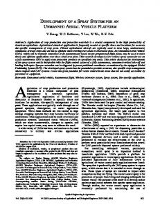
article is promising. Figures 8 show the paths found by the proposed algorithms for a Dubins’ instance.

Length (m)

50 instances were generated and all the targets were chosen randomly from a square area of 5000 × 5000 units. In addition, all the instances of the problem have 5 depots chosen at fixed locations in the square area. All the simulations were run on a Dell Precision T5500 workstation (Intel Xeon E5630 processor @ 2.53GHz, 12GB RAM). The simulations were performed for a fixed wing vehicle with minimum turning radius constraints. A vehicle traveling at a constant speed with a bound on its turning radius is referred to as the Dubins’ vehicle [6]. In the simulations, the minimum turning radius of the vehicle is chosen to be 100 units and the angle of approach for each target is selected uniformly in the interval [0, 2π] radians. Given the approach angles at the targets, the minimum distance required to travel between any two targets subject to the turning radius constraints of the vehicle was solved by Dubins in [6]. For the simulations, the maximum fuel capacity L was 4500 units and we assumed that the fuel spent is directly proportional to the distance traveled by the vehicle. The formulation presented in section V was solved to optimality using IBM ILOG CPLEX optimization software [22]. The average time required to find an optimal solution in CPLEX was nearly 2 hours for problem instances with 25 targets and 5 depots. On the other hand, the average time required to find a feasible solution using the approximation algorithm and the heuristics was less than 2 seconds for each tested instance. The quality of a solution produced by applying an algorithm on

2500 2000 1500 1000 500

0

1000

2000

3000

Length (m)

4000

5000

(d)Solution found by using CPLEX after 10 seconds with the solution in (b) as an initial feasible solution Fig. 8. The paths found by the algorithms for a Dubins’ instance with 25 nodes.

9 50

Deviation from Optimum (%)

45 40 35

Approximation algorithm Construction heuristic Improvement heuristic CPLEX with initial feasible solution in10s

30 25 20 15 10 5 0

10

15

Number of Targets

20

25

Fig. 9. Average quality of solutions produced by the proposed algorithms.

VII. C ONCLUSIONS An approximation algorithm and fast heuristics were developed to solve a generalization of the single vehicle routing problem with fuel constraints. A mixed-integer, linear programming formulation was also proposed to find optimal solutions to the problem. Future work can be directed towards developing branch and cut methods, and can address problems with multiple, heterogeneous vehicles. R EFERENCES [1] [2] [3] [4]

[5] [6]

[7] [8] [9] [10]

[11] [12]

[13]

T. Zajkowski, S. Dunagan, and J. Eilers, “Small UAS communications mission,” in Eleventh Biennial USDA Forest Service Remote Sensing Applications Conference, Salt Lake City, UT, 2006. E. W. Frew and T. X. Brown, “Networking issues for small unmanned aircraft systems,” Unmanned Aircraft Systems, pp. 21–37, 2009. J. A. Curry, J. Maslanik, G. Holland, J. Pinto, G. Tyrrell, and J. Inoue, “Applications of aerosondes in the arctic,” Bull. Am. Meteorol. Soc, vol. 85, no. 12, pp. 1855–1861, 2004. C. E. Corrigan, G. C. Roberts, M. V. Ramana, D. Kim, V. Ramanathan, et al., “Capturing vertical profiles of aerosols and black carbon over the indian ocean using autonomous unmanned aerial vehicles,” Atmospheric Chemistry and Physics, vol. 8, no. 3, pp. 737–747, 2008. “Soldiers train with raven UAV’s, united states army.” [Online]. Available: http://www.army.mil/article/5644/soldiers-train-with-raven-uavs/ L. E. Dubins, “On curves of minimal length with a constraint on average curvature, and with prescribed initial and terminal positions and tangents,” American Journal of Mathematics, vol. 79, no. 3, pp. 497–516, July 1957, ArticleType: research-article / Full publication date: Jul., 1957 / Copyright 1957 The Johns Hopkins University Press. A. M. Frieze, G. Galbiati, and F. Maffioli, “On the worst-case performance of some algorithms for the asymmetric traveling salesman problem,” Networks, vol. 12, no. 1, pp. 23–39, 1982. H. Kaplan, M. Lewenstein, N. Shafrir, and M. Sviridenko, “Approximation algorithms for asymmetric TSP by decomposing directed regular multigraphs,” Journal of the ACM (JACM), vol. 52, no. 4, pp. 602–626, 2005. M. Blaser, “A new approximation algorithm for the asymmetric TSP with triangle inequality,” ACM Transactions on Algorithms (TALG), vol. 4, no. 4, p. 47, 2008. S. Khuller, A. Malekian, and J. Mestre, “To fill or not to fill: The gas station problem,” in Algorithms ESA 2007, L. Arge, M. Hoffmann, and E. Welzl, Eds. Berlin, Heidelberg: Springer Berlin Heidelberg, 2007, vol. 4698, pp. 534–545. P. B. Sujit and D. Ghose, “Two-agent cooperative search using game models with endurance-time constraints,” Engineering Optimization, vol. 42, no. 7, pp. 617–639, 2010. G. Ghiani, F. Guerriero, G. Laporte, and R. Musmanno, “Tabu search heuristics for the arc routing problem with intermediate facilities under capacity and length restrictions,” Journal of Mathematical Modelling and Algorithms, vol. 3, no. 3, pp. 209–223, 2004. M. Polacek, K. F. Doerner, R. F. Hartl, and V. Maniezzo, “A variable neighborhood search for the capacitated arc routing problem with intermediate facilities,” Journal of Heuristics, vol. 14, no. 5, pp. 405–423, 2008.

[14] E. Angelelli and M. Grazia Speranza, “The periodic vehicle routing problem with intermediate facilities,” European Journal of Operational Research, vol. 137, no. 2, pp. 233–247, 2002. [15] B. Crevier, J. F. Cordeau, and G. Laporte, “The multi-depot vehicle routing problem with inter-depot routes,” European Journal of Operational Research, vol. 176, no. 2, pp. 756–773, 2007. [16] E. D. Taillard, G. Laporte, and M. Gendreau, “Vehicle routeing with multiple use of vehicles,” The Journal of the Operational Research Society, vol. 47, no. 8, pp. pp. 1065–1070, 1996. [17] Q. H. Zhao, S. Y. Wang, K. K. Lai, and G. Xia, “A vehicle routing problem with multiple use of vehicles,” Advanced Modeling and Optimization, vol. 4, no. 3, pp. 21–40, 2002. [18] J. O. Royset, W. M. Carlyle, and R. K. Wood, “Routing military aircraft with a constrained shortest-path algorithm,” Military Operations Research, vol. 14, no. 3, pp. 31–52, 2009. [19] E. W. Dijkstra, “A note on two problems in connexion with graphs,” Numerische mathematik, vol. 1, no. 1, pp. 269–271, 1959. [20] S.-H. Lin, “Finding optimal refueling policies in transportation networks,” in Algorithmic Aspects in Information and Management, R. Fleischer and J. Xu, Eds. Berlin, Heidelberg: Springer Berlin Heidelberg, 2008, vol. 5034, pp. 280–291. [21] T. Magnanti and L. Wolsey, “Optimal trees,” Universit catholique de Louvain, Center for Operations Research and Econometrics (CORE), Tech. Rep., Jan. 1994. [22] “IBM - ILOG: CPLEX optimization studio 12.2.” [Online]. Available: http://www.ilog.com/products/cplex [23] “Python programming language (v.2.7.2).” [Online]. Available: http://www.python.org/psf/