faster than Strassen's algorithm, and contains proofs that matrix multiplication, matrix squaring ..... 5.1 A Plot of M4RI's System Solving in Sage vs Magma . . . . . . . . . 104 .... a Java library for converting polynomials into Cnf-Sat problems.
ABSTRACT
Title of dissertation:
ALGORITHMS FOR SOLVING LINEAR AND POLYNOMIAL SYSTEMS OF EQUATIONS OVER FINITE FIELDS WITH APPLICATIONS TO CRYPTANALYSIS Gregory Bard Doctor of Philosophy, 2007
Dissertation directed by:
Professor Lawrence C. Washington Department of Mathematics
This dissertation contains algorithms for solving linear and polynomial systems of equations over GF(2). The objective is to provide fast and exact tools for algebraic cryptanalysis and other applications. Accordingly, it is divided into two parts. The first part deals with polynomial systems. Chapter 2 contains a successful cryptanalysis of Keeloq, the block cipher used in nearly all luxury automobiles. The attack is more than 16,000 times faster than brute force, but queries 0.6 × 232 plaintexts. The polynomial systems of equations arrising from that cryptanalysis were solved via SAT-solvers. Therefore, Chapter 3 introduces a new method of solving polynomial systems of equations by converting them into CNF-SAT problems and using a SAT-solver. Finally, Chapter 4 contains a discussion on how SAT-solvers work internally. The second part deals with linear systems over GF(2), and other small fields (and rings). These occur in cryptanalysis when using the XL algorithm, which con-
verts polynomial systems into larger linear systems. We introduce a new complexity model and data structures for GF(2)-matrix operations. This is discussed in Appendix B but applies to all of Part II. Chapter 5 contains an analysis of “the Method of Four Russians” for multiplication and a variant for matrix inversion, which is log n faster than Gaussian Elimination, and can be combined with Strassen-like algorithms. Chapter 6 contains an algorithm for accelerating matrix multiplication over small finite fields. It is feasible but the memory cost is so high that it is mostly of theoretical interest. Appendix A contains some discussion of GF(2)-linear algebra and how it differs from linear algebra in R and C. Appendix C discusses algorithms faster than Strassen’s algorithm, and contains proofs that matrix multiplication, matrix squaring, triangular matrix inversion, LUP-factorization, general matrix inversion and the taking of determinants, are equicomplex. These proofs are already known, but are here gathered into one place in the same notation.
ALGORITHMS FOR SOLVING LINEAR AND POLYNOMIAL SYSTEMS OF EQUATIONS OVER FINITE FIELDS, WITH APPLICATIONS TO CRYPTANALYSIS
by Gregory V. Bard
Dissertation submitted to the Faculty of the Graduate School of the University of Maryland, College Park in partial fulfillment of the requirements for the degree of Doctor of Philosophy 2007
Advisory Committee: Professor Lawrence C. Washington, Chair/Advisor Professor William Adams, Professor Steven Tretter, Professor William Gasarch, Assistant Professor Jonathan Katz.
© Copyright by
Gregory V. Bard 2007
Preface Pigmaei gigantum humeris impositi plusquam ipsi gigantes vident1 . (Attributed to Bernard of Chartres, ) One of the many reasons the subject of Mathematics is so beautiful is the continuing process of building one theorem, algorithm, or conjecture upon another. This can be compared to the construction of a cathedral, where each stone gets laid upon those that came before it with great care. As each mason lays his stone he can only be sure to put it in its proper place, and see that it rests plumb, level, and square, with its neighbors. From that vantage point, it is impossible to tell what role it will play in the final edifice, or even if it will be visible. Could George Boole have imagined the digital computer? Another interesting point is that the cathedrals of Europe almost universally took longer than one lifetime to build. Therefore those that laid the foundations had absolutely no probability at all of seeing the completed work. This is true in mathematics, also. Fermat’s Last Theorem, the Kepler Conjecture, the Insolubility of the Quintic, the Doubling of the Cube, and other well-known problems were only solved several centuries after they were proposed. And thus scholarly publication is a great bridge, which provides communication of ideas (at least in one direction) across the abyss of death. On example is to contemplate the conic sections of Apollonius of Perga, (circa bc). Can one imagine how few of the ordinary or extraordinary persons of Western Europe in perhaps the seventh century ad, would know of them. Yet, centuries after their introduction, they would be found, by Kepler, to describe the motions of astronomical bodies. In the late twentieth century, conic sections were studied, at least to some degree, by all high school graduates in the United States of America, and certainly other countries as well. Such is the nature of our business. Some papers might be read by only ten persons in a century. All we can do is continue to work, and hope that the knowledge we create is used for good and not for ill. An old man, going a lone highway, Came at the evening, cold and gray, To a chasm, vast and deep and wide, Through which was flowing a sullen tide. The old man crossed in the twilight dim; The sullen stream had no fears for him; But he turned when safe on the other side And built a bridge to span the tide. “Old man,” said a fellow pilgrim near, “You are wasting strength with building here; Your journey will end with the ending day; You never again must pass this way; 1
Dwarves, standing on the shoulders of giants, can further than giants see.
ii
You have crossed the chasm, deep and wide— Why build you the bridge at the eventide?” The builder lifted his old gray head: “Good friend, in the path I have come,” he said, “There followeth after me today A youth whose feet must pass this way. This chasm that has been naught to me To that fair-haired youth may a pitfall be. He, too, must cross in the twilight dim; Good friend, I build this bridge for him.” by William Allen Drumgoole
iii
Foreword The ignoraunte multitude doeth, but as it was euer wonte, enuie that knoweledge, whiche thei can not attaine, and wishe all men ignoraunt, like unto themself. . . Yea, the pointe in Geometrie, and the unitie in Arithmetike, though bothe be undiuisible, doe make greater woorkes, & increase greater multitudes, then the brutishe bande of ignoraunce is hable to withstande. . . But yet one commoditie moare. . . I can not omitte. That is the filying, sharpenyng, and quickenyng of the witte, that by practice of Arithmetike doeth insue. It teacheth menne and accustometh them, so certainly to remember thynges paste: So circumspectly to consider thynges presente: And so prouidently to forsee thynges that followe: that it maie truelie bee called the File of witte. (Robert Recorde, , quoted from [vzGG03, Ch. 17]).
iv
Dedication With pleasure, I dedicate this dissertation to my parents. To my father, who taught me much in mathematics, most especially calculus, years earlier than I would have been permitted to see it. And to my mother, who has encouraged me in every endeavor.
v
Acknowledgments I am deeply indebted to my advisor, Professor Lawrence C. Washington, who has read and re-read many versions of this document, and every other research paper I have written to date, provided me with countless hours of his time, and given me sound advice, on matters technical, professional and personal. He has had many students, and all I have spoken to are in agreement that he is a phenomenal advisor, and it is humbling to know that we can never possibly equal him. We can only try to emulate him. I have been very fortunate to work with Dr. Nicolas T. Courtois, currently Senior Lecturer at the University College of London. It suffices to say that the field of algebraic cryptanalysis has been revolutionized by his work.
He permitted me
to study with him for four months in Paris, and later even to stay at his home in England. Much of my work is joint work with him. My most steadfast supporter has been my best friend and paramour, Patrick Studdard. He has read every paper I have written to date, even this dissertation. He has listened to me drone on about topics like group theory or ring theory and has tolerated my workaholism. My life and my work would be much more empty without him. My first autonomous teaching experience was at American University, a major stepping stone in my life. The Department of Computer Science, Audio Technology and Physics had faith in me and put their students in my hands. I am so very grateful for those opportunities. In particular I would like to thank Professor Michael Gray,
vi
and Professor Angela Wu, who gave me much advice. The departmental secretary, Yana Shabaev was very kind to me on numerous occasions and I am grateful for all her help. I also received valuable teaching advice from my future father-inlaw, Emeritus Professor Albert Studdard, of the Philosophy Department at the University of North Carolina at Pembroke. My admission to the Applied Mathematics and Scientific Computation (AMSC) Program at the University of Maryland was unusual. I had been working as a PhD student in Computer Engineering for several years when I decided to add a Masters in AMSC as a side task. Later, I switched, and made it the focus of my PhD. Several faculty members were important in helping me make that transition, including Professor Virgil D. Gligor, Professor Richard Schwartz, and Professor Jonathan Rosenberg. But without the program chair, Professor David Levermore, and my advisor, Professor Lawrence C. Washington, this would have been impossible. I am grateful that many rules were bent. Several governmental agencies have contributed to my education. In reverse chronological order, The National Science Foundation (NSF) VIGRE grant to the University of
Maryland provided the Mathematics Department with funds for “Dissertation Completion Fellowships.” These are exceedingly generous semester-long gifts and I had the pleasure to receive two of them. I am certain this dissertation would look very different without that valuable support. I furthermore received travel funding and access to super-computing under the
vii
NSF grant for the Sage project [sag], Grant Number 0555776. The European Union established the ECRYPT organization to foster research
among cryptographers. The ECRYPT foundation was kind enough to support me during my research visit in Paris. Much of the work of this dissertation was done while working there. The Department of the Navy, Naval Sea Systems Command, Carderock Sta-
tion, supported me with a fascinating internship during the summer of 2003. They furthermore allowed me to continue some cryptologic research toward my graduate degrees while working there. The National Security Agency was my employer from May of 1998 until
September of 2002. Not only did I have the chance to work alongside and learn from some of the most dedicated and professional engineers, computer scientists and mathematicians who have ever been assembled into one organization, but also I was given five semesters of financial support, plus several summer sessions, which was very generous, especially considering that two of those semesters and one summer were during wartime. Our nation owes an enormous debt to the skill, perseverance, self-discipline, and creativity of the employees of the National Security Agency. Several employees there were supporters of my educational hopes but security regulations and agency traditions would forbid my mentioning them by name. Professor Virgil D. Gligor, Professor Jonathan Katz, and Professor William R. Franklin (of RPI), have all been my academic advisor at one time or another viii
and I thank them for their guidance. Each has taught me from their own view of computer security and it is interesting how many points of view there really are. Our field is enriched by this diversity of scholarly background. Likewise Dr Harold Snider gave me important advice during my time at Oxford. My Oxford days were an enormous influence on my decision to switch into Applied Mathematics from Computer Engineering. My alma mater, the Rensselaer Polytechnic Institute, has furnished me with many skills. I cannot imagine a better training ground. My engineering degree was sufficiently mathematically rigorous that I succeeded in a graduate program in Applied Mathematics, without having a Bachelor’s degree in Mathematics. In fact, only two courses, Math 403, Abstract Algebra, and Math 404 Field Theory, were my transition. Yet I was practical enough to hired into and promoted several times at the NSA, from a Grade 6 to a Grade 11 (out of a maximum of 15), including several commendations and a Director’s Star. I am particularly indebted to the faculty there, and its founder, Stephen Van Rensselaer, former governor of New York and (twice) past Grand Master of Free & Accepted Masons of the State of New York. It was at Rensselaer that I learned of and was initiated into Freemasonry, and the Institute’s mission of educating “the sons of farmers and mechanics” with “knowledge and thoroughness” echoes the teachings of Freemasonry. My two greatest friends, chess partners, and Brother Freemasons, Paul Bello and Abram Claycomb, were initiated there as well, and I learned much in discussions with them. I learned of cryptography at a very young age, perhaps eight years old or so. Dr. Haig Kafafian, also a Freemason and a family friend, took me aside after Church ix
for many years and taught me matrices, classical cryptography, and eventually, allowed me to be an intern at his software development project to make devices to aid the handicapped. There I met Igor Kalatian, who taught me the C language. I am grateful to them both.
x
Table of Contents List of Tables
xv
List of Figures
xvii
List of Abbreviations
xix
1 Summary
1
I Polynomial Systems
5
2 An 2.1 2.2 2.3
Extended Example: The Block-Cipher Keeloq Special Acknowledgment of Joint Work . . . . . . Notational Conventions and Terminology . . . . . The Formulation of Keeloq . . . . . . . . . . . . . 2.3.1 What is Algebraic Cryptanalysis? . . . . . 2.3.2 The CSP Model . . . . . . . . . . . . . . . 2.3.3 The Keeloq Specification . . . . . . . . . . 2.3.4 Modeling the Non-linear Function . . . . . 2.3.5 I/O Relations and the NLF . . . . . . . . 2.3.6 Disposing of the Secret Key Shift-Register 2.3.7 Describing the Plaintext Shift-Register . . 2.3.8 The Polynomial System of Equations . . . 2.3.9 Variable and Equation Count . . . . . . . 2.3.10 Dropping the Degree to Quadratic . . . . 2.3.11 Fixing or Guessing Bits in Advance . . . . 2.3.12 The Failure of a Frontal Assault . . . . . . 2.4 Our Attack . . . . . . . . . . . . . . . . . . . . . 2.4.1 A Particular Two Function Representation (8) 2.4.2 Acquiring an fk -oracle . . . . . . . . . . 2.4.3 The Consequences of Fixed Points . . . . . 2.4.4 How to Find Fixed Points . . . . . . . . . 2.4.5 How far must we search? . . . . . . . . . . 2.4.6 Fraction of Plainspace Required . . . . . . 2.4.7 Comparison to Brute Force . . . . . . . . 2.4.8 Some Lemmas . . . . . . . . . . . . . . . . 2.4.9 Cycle Lengths in a Random Permutation . 2.5 Summary . . . . . . . . . . . . . . . . . . . . . . 2.6 A Note about Keeloq’s Utilization . . . . . . . . .
xi
. . . . . . . . . . . . . . . . . . . . . . . . . . .
. . . . . . . . . . . . . . . . . . . . . . . . . . .
. . . . . . . . . . . . . . . . . . . . . . . . . . .
. . . . . . . . . . . . . . . . . . . . . . . . . . .
. . . . . . . . . . . . . . . . . . . . . . . . . . .
. . . . . . . . . . . . . . . . . . . . . . . . . . .
. . . . . . . . . . . . . . . . . . . . . . . . . . .
. . . . . . . . . . . . . . . . . . . . . . . . . . .
. . . . . . . . . . . . . . . . . . . . . . . . . . .
. . . . . . . . . . . . . . . . . . . . . . . . . . .
. . . . . . . . . . . . . . . . . . . . . . . . . . .
6 7 7 8 8 8 9 10 11 12 12 13 14 14 16 16 18 18 18 19 20 22 23 25 26 29 32 34
3 Converting MQ to CNF-SAT 3.1 Summary . . . . . . . . . . . . . . . . . . . . . 3.2 Introduction . . . . . . . . . . . . . . . . . . . . 3.2.1 Application to Cryptanalysis . . . . . . . 3.3 Notation and Definitions . . . . . . . . . . . . . 3.4 Converting MQ to SAT . . . . . . . . . . . . . . 3.4.1 The Conversion . . . . . . . . . . . . . . 3.4.1.1 Minor Technicality . . . . . . . 3.4.2 Measures of Efficiency . . . . . . . . . . 3.4.3 Preprocessing . . . . . . . . . . . . . . . 3.4.4 Fixing Variables in Advance . . . . . . . 3.4.4.1 Parallelization . . . . . . . . . 3.4.5 SAT-Solver Used . . . . . . . . . . . . . 3.4.5.1 Note About Randomness . . . 3.5 Experimental Results . . . . . . . . . . . . . . . 3.5.1 The Source of the Equations . . . . . . . 3.5.2 The Log-Normal Distribution of Running 3.5.3 The Optimal Cutting Number . . . . . . 3.5.4 Comparison with MAGMA, Singular . . 3.6 Previous Work . . . . . . . . . . . . . . . . . . 3.7 Conclusions . . . . . . . . . . . . . . . . . . . . 3.8 Cubic Systems . . . . . . . . . . . . . . . . . . . 3.9 NP-Completeness of MQ . . . . . . . . . . . . .
. . . . . . . . . . . . . . . . . . . . . . . . . . . . . . . . . . . . . . . . . . . . . . . . . . . . . . . . . . . . Times . . . . . . . . . . . . . . . . . . . . . . . .
. . . . . . . . . . . . . . . . . . . . . .
. . . . . . . . . . . . . . . . . . . . . .
. . . . . . . . . . . . . . . . . . . . . .
. . . . . . . . . . . . . . . . . . . . . .
. . . . . . . . . . . . . . . . . . . . . .
. . . . . . . . . . . . . . . . . . . . . .
. . . . . . . . . . . . . . . . . . . . . .
. . . . . . . . . . . . . . . . . . . . . .
35 35 36 37 39 40 40 40 43 45 46 48 48 48 49 50 50 52 55 55 57 57 60
4 How do SAT-Solvers Operate? 4.1 The Problem Itself . . . . . . . . . . . . . . 4.1.1 Conjunctive Normal Form . . . . . . 4.2 Chaff and its Descendants . . . . . . . . . . 4.2.1 Variable Management . . . . . . . . . 4.2.2 The Method of Watched Literals . . 4.2.3 How to Actually Make This Happen 4.2.4 Back-Tracking . . . . . . . . . . . . . 4.3 Enhancements to Chaff . . . . . . . . . . . . 4.3.1 Learning . . . . . . . . . . . . . . . . 4.3.2 The Alarm Clock . . . . . . . . . . . 4.3.3 The Third Finger . . . . . . . . . . . 4.4 Walk-SAT . . . . . . . . . . . . . . . . . . . 4.5 Economic Motivations . . . . . . . . . . . .
. . . . . . . . . . . . .
. . . . . . . . . . . . .
. . . . . . . . . . . . .
. . . . . . . . . . . . .
. . . . . . . . . . . . .
. . . . . . . . . . . . .
. . . . . . . . . . . . .
. . . . . . . . . . . . .
. . . . . . . . . . . . .
62 62 63 64 64 66 66 68 70 70 71 71 72 72
II Linear Systems
. . . . . . . . . . . . .
. . . . . . . . . . . . .
. . . . . . . . . . . . .
. . . . . . . . . . . . .
. . . . . . . . . . . . .
74
5 The Method of Four Russians 75 5.1 Origins and Previous Work . . . . . . . . . . . . . . . . . . . . . . . . 76 5.1.1 Strassen’s Algorithm . . . . . . . . . . . . . . . . . . . . . . . 77 xii
5.2 5.3
Rapid Subspace Enumeration . . . . . . . . . . . . . . . . . The Four Russians Matrix Multiplication Algorithm . . . . . 5.3.1 Role of the Gray Code . . . . . . . . . . . . . . . . . 5.3.2 Transposing the Matrix Product . . . . . . . . . . . . 5.3.3 Improvements . . . . . . . . . . . . . . . . . . . . . . 5.3.4 A Quick Computation . . . . . . . . . . . . . . . . . 5.3.5 M4RM Experiments Performed by SAGE Staff . . . . 5.4 The Four Russians Matrix Inversion Algorithm . . . . . . . . 5.4.1 Stage 1: . . . . . . . . . . . . . . . . . . . . . . . . . 5.4.2 Stage 2: . . . . . . . . . . . . . . . . . . . . . . . . . 5.4.3 Stage 3: . . . . . . . . . . . . . . . . . . . . . . . . . 5.4.4 A Curious Note on Stage 1 of M4RI . . . . . . . . . . 5.4.5 Triangulation or Inversion? . . . . . . . . . . . . . . . 5.5 Experimental and Numerical Results . . . . . . . . . . . . . 5.6 Exact Analysis of Complexity . . . . . . . . . . . . . . . . . 5.6.1 An Alternative Computation . . . . . . . . . . . . . . 5.6.2 Full Elimination, not Triangular . . . . . . . . . . . . 5.6.3 The Rank of 3k Rows, or Why k + � is not Enough . 5.6.4 Using Bulk Logical Operations . . . . . . . . . . . . . 5.6.5 M4RI Experiments Performed by SAGE Staff . . . . 5.6.5.1 Determination of k . . . . . . . . . . . . . . 5.6.5.2 Comparison to Magma . . . . . . . . . . . . 5.6.5.3 The Transpose Experiment . . . . . . . . . 5.7 Pairing With Strassen’s Algorithm for Matrix Multiplication 5.8 The Unsuitability of Strassen’s Algorithm for Inversion . . . 5.8.1 Bunch and Hopcroft’s Solution . . . . . . . . . . . . 5.8.2 Ibara, Moran, and Hui’s Solution . . . . . . . . . . .
. . . . . . . . . . . . . . . . . . . . . . . . . . .
. . . . . . . . . . . . . . . . . . . . . . . . . . .
. . . . . . . . . . . . . . . . . . . . . . . . . . .
. . . . . . . . . . . . . . . . . . . . . . . . . . .
. . . . . . . . . . . . . . . . . . . . . . . . . . .
78 80 81 82 82 82 83 84 86 86 86 87 90 91 96 97 98 99 101 102 102 102 103 103 105 107 108
6 An Impractical Method of Accelerating Matrix Operations in Rings of Finite Size 113 6.1 Introduction . . . . . . . . . . . . . . . . . . . . . . . . . . . . . . . . 113 6.1.1 Feasibility . . . . . . . . . . . . . . . . . . . . . . . . . . . . . 114 6.2 The Algorithm over a Finite Ring . . . . . . . . . . . . . . . . . . . . 115 6.2.1 Summary . . . . . . . . . . . . . . . . . . . . . . . . . . . . . 116 6.2.2 Complexity . . . . . . . . . . . . . . . . . . . . . . . . . . . . 116 6.2.3 Taking Advantage of z 6= 1 . . . . . . . . . . . . . . . . . . . . 118 6.2.4 The Transpose of Matrix Multiplication . . . . . . . . . . . . 118 6.3 Choosing Values of b . . . . . . . . . . . . . . . . . . . . . . . . . . . 119 6.3.1 The “Conservative” Algorithm . . . . . . . . . . . . . . . . . . 119 6.3.2 The “Liberal” Algorithm . . . . . . . . . . . . . . . . . . . . . 120 6.3.3 Comparison . . . . . . . . . . . . . . . . . . . . . . . . . . . . 122 6.4 Over Finite Fields . . . . . . . . . . . . . . . . . . . . . . . . . . . . . 122 6.4.1 Complexity Penalty . . . . . . . . . . . . . . . . . . . . . . . . 123 6.4.2 Memory Requirements . . . . . . . . . . . . . . . . . . . . . . 123 6.4.3 Time Requirements . . . . . . . . . . . . . . . . . . . . . . . . 124 xiii
6.5 6.6 6.7
6.4.4 The Conservative Algorithm 6.4.5 The Liberal Algorithm . . . Very Small Finite Fields . . . . . . Previous Work . . . . . . . . . . . Notes . . . . . . . . . . . . . . . . . 6.7.1 Ring Additions . . . . . . . 6.7.2 On the Ceiling Symbol . . .
. . . . . . .
. . . . . . .
. . . . . . .
. . . . . . .
. . . . . . .
. . . . . . .
. . . . . . .
. . . . . . .
A Some Basic Facts about Linear Algebra over GF(2) A.1 Sources . . . . . . . . . . . . . . . . . . . . . . . . A.2 Boolean Matrices vs GF(2) Matrices . . . . . . . A.3 Why is GF(2) Different? . . . . . . . . . . . . . . A.3.1 There are Self-Orthogonal Vectors . . . . . A.3.2 Something that Fails . . . . . . . . . . . . A.3.3 The Probability a Random Square Matrix vertible . . . . . . . . . . . . . . . . . . .
. . . . . . .
. . . . . . .
. . . . . . .
. . . . . . .
. . . . . . .
. . . . . . .
. . . . . . .
. . . . . . .
. . . . . . . . . . . . . . . . . . . . . . . . . . . . . . . . . . . . . . . . is Singular or . . . . . . . .
. . . . . . .
. . . . . . .
. . . . . . .
124 125 125 128 128 128 129
. . . . .
131 131 131 131 132 132
. . . . . . . . . . In. .
. 133
B A Model for the Complexity of GF(2)-Operations B.1 The Cost Model . . . . . . . . . . . . . . . . . . . . . B.1.1 Is the Model Trivial? . . . . . . . . . . . . . . B.1.2 Counting Field Operations . . . . . . . . . . . B.1.3 Success and Failure . . . . . . . . . . . . . . . B.2 Notational Conventions . . . . . . . . . . . . . . . . . B.3 To Invert or to Solve? . . . . . . . . . . . . . . . . . B.4 Data Structure Choices . . . . . . . . . . . . . . . . . B.4.1 Dense Form: An Array with Swaps . . . . . . B.4.2 Permutation Matrices . . . . . . . . . . . . . . B.5 Analysis of Classical Techniques with our Model . . . B.5.1 Na¨ıve Matrix Multiplication . . . . . . . . . . B.5.2 Matrix Addition . . . . . . . . . . . . . . . . B.5.3 Dense Gaussian Elimination . . . . . . . . . . B.5.4 Strassen’s Algorithm for Matrix Multiplication
. . . . . . . . . . . . . .
. . . . . . . . . . . . . .
. . . . . . . . . . . . . .
. . . . . . . . . . . . . .
. . . . . . . . . . . . . .
. . . . . . . . . . . . . .
. . . . . . . . . . . . . .
. . . . . . . . . . . . . .
. . . . . . . . . . . . . .
135 135 136 136 137 137 138 138 139 139 140 140 140 140 142
C On the Exponent of Certain Matrix Operations C.1 Very Low Exponents . . . . . . . . . . . . C.2 The Equicomplexity Theorems . . . . . . . C.2.1 Starting Point . . . . . . . . . . . . C.2.2 Proofs . . . . . . . . . . . . . . . . C.2.3 A Common Misunderstanding . . .
. . . . .
. . . . .
. . . . .
. . . . .
. . . . .
. . . . .
. . . . .
. . . . .
. . . . .
145 145 146 147 147 153
Bibliography
. . . . .
. . . . .
. . . . .
. . . . .
. . . . .
. . . . .
154
xiv
List of Tables
2.1
Fixed points of random permutations and their 8th powers . . . . . . 22
3.1
CNF Expression Difficulty Measures for Quadratic Systems, by Cutting Number . . . . . . . . . . . . . . . . . . . . . . . . . . . . . . . . 45
3.2
Running Time Statistics in Seconds . . . . . . . . . . . . . . . . . . . 54
3.3
Speeds of Comparison Trials between Magma, Singular and ANFtoCNFMiniSAT . . . . . . . . . . . . . . . . . . . . . . . . . . . . . . . . . . 56
3.4
CNF Expression Difficulty Measures for Cubic Systems, by Cutting Number . . . . . . . . . . . . . . . . . . . . . . . . . . . . . . . . . . 59
5.1
M4RM Running Times versus Magma . . . . . . . . . . . . . . . . . 84
5.2
Confirmation that k = 0.75 log2 n is not a good idea. . . . . . . . . . 84
5.3
Probabilities of a Fair-Coin Generated n × n matrix over GF(2), having given Nullity . . . . . . . . . . . . . . . . . . . . . . . . . . . . . 91
5.4
Experiment 1— Optimal Choices of k, and running time in seconds. . 94
5.5
Running times, in msec, Optimization Level 0 . . . . . . . . . . . . . 94
5.6
Percentage Error for Offset of K, From Experiment 1 . . . . . . . . . 95
5.7
Results of Experiment 3—Running Times, Fixed k=8 . . . . . . . . . 110
5.8
Experiment 2—Running times in seconds under different Optimizations, k=8 . . . . . . . . . . . . . . . . . . . . . . . . . . . . . . . . . 110
5.9
Trials between M4RI and Gaussian Elimination (msec) . . . . . . . . 111
5.10 The Ineffectiveness of the Transpose Trick . . . . . . . . . . . . . . . 111 5.11 Optimization Level 3, Flexible k . . . . . . . . . . . . . . . . . . . . . 112 6.1
The Speed-Up and Extra Memory Usage given by the four choices . . 126
6.2
Memory Required (in bits) and Speed-Up Factor (w/Strassen) for Various Rings . . . . . . . . . . . . . . . . . . . . . . . . . . . . . . . 127
xv
B.1 Algorithms and Performance, for m × n matrices . . . . . . . . . . . 144
xvi
List of Figures
2.1
The Keeloq Circuit Diagram . . . . . . . . . . . . . . . . . . . . . . .
9
3.1
The Distribution of Running Times, Experiment 1 . . . . . . . . . . . 51
3.2
The Distribution of the Logarithm of Running Times, Experiment 1 . 52
5.1
A Plot of M4RI’s System Solving in Sage vs Magma . . . . . . . . . 104
C.1 The Relationship of the Equicomplexity Proofs . . . . . . . . . . . . . 147
xvii
List of Algorithms 1 2 3 4 5 6 7 8 9 10 11
Method of Four Russians, for Matrix Multiplication . Method of Four Russians, for Inversion . . . . . . . . The Finite-Ring Algorithm . . . . . . . . . . . . . . . Fast Mb (R) multiplications for R a finite field but not Gram-Schmidt, over a field of characteristic zero. . . To compose two row swap arrays r and s, into t . . . To invert a row swap array r, into s . . . . . . . . . . Na¨ıve Matrix Multiplication . . . . . . . . . . . . . . Dense Gaussian Elimination, for Inversion . . . . . . Dense Gaussian Elimination, for Triangularization . . Strassen’s Algorithm for Matrix Multiplication . . . .
xviii
. . . . . . . . . . . . GF(2) . . . . . . . . . . . . . . . . . . . . . . . . . . . .
. . . . . . . . . . .
. . . . . . . . . . .
. . . . . . . . . . .
. . . . . . . . . . .
. . . . . . . . . . .
80 85 116 123 132 139 140 140 141 142 142
List of Abbreviations (x) f (x) = o(g(x)) limx→∞ fg(x) =0 f (x) = O(g(x)) ∃c, n0 ∀n > n0 f (x) = Ω(g(x)) ∃c, n0 ∀n > n0 g(x) f (x) = ω(g(x)) limx→∞ f (x) = 0
f (x) ≤ cg(x) f (x) ≥ cg(x)
f (x) = Θ(g(x))
f (x) = O(g(x)) while simultaneously f (x) = Ω(g(x))
f (x) ∼ g(x)
limx→∞
Cnf-Sat Des GF(q) Hfe M4rm M4ri Mc Mq Owf Quad Rref Sage Sat Uutf
The conjunctive normal form satisfiability problem The Data Encryption Standard The finite field of size q Hidden Field Equations (a potential trap-door OWF) The Method of Four Russians for matrix multiplication The Method of Four Russians for matrix inversion The Multivariate Cubic problem The Multivariate Quadratic problem One-way Function The stream cipher defined in [BGP05] Reduced Row Echelon Form Software for Algebra and Geometry Experimentation The satisfiability problem Unit Upper Triangular Form
f (x) g(x)
=1
xix
Chapter 1 Summary Generally speaking, it has been the author’s objective to generate efficient and reliable computational tools to assist algebraic cryptanalysts. In practice, this is a question of developing tools for systems of equations, which may be dense or sparse, linear or polynomial, over GF(2) or one of its extension fields. In addition, the author has explored the cryptanalysis of block ciphers and stream ciphers, targeting the block ciphers Keeloq and the Data Encryption Standard (Des), and the stream cipher Quad. Only Keeloq is presented here, because the work on the last two are still underway. The work on Des has seen preliminary publication in [CB06]. The dissertation is divided into two parts. The first deals with polynomial systems and actual cryptanalysis. The second deals with linear systems. Linear systems are important to cryptanalysis because of the XL algorithm [CSPK00], a standard method of solving overdefined polynomial systems of equations over finite fields by converting them into linear systems. Chapter 2 is the most practical, and contains a detailed study of the block cipher Keeloq and presents a successful algebraic cryptanalysis attack. The cipher Keeloq is used in the key-less entry systems of nearly all luxury automobiles. Our attack is 214.77 times faster than brute force, but requires 0.6 × 232 plaintexts. Chapter 3 has the largest potential future impact, and deals not with linear
1
systems but with polynomial systems. Also, it deals not only with dense systems (as Part II does), but with sparse systems also. Since it is known that solving a quadratic system of equations is NP-hard, and solving the Cnf-Sat problem is NPhard, and since all NP-Complete problems are polynomially reducible to each other, it makes sense to look for a method to use one in solving the other. This chapter shows how to convert quadratic systems of equations into Cnf-Sat problems, and that using off-the-shelf Sat-solvers is an efficient method of solving this difficult problem. Chapter 4 describes in general terms how Sat-solvers work. This tool is often viewed as a black box, which is unfortunate. There is no novel work in this chapter, except the author does not know of any other exposition on how these tools operate, either for experts or a general audience. The second part begins with Chapter 5, and contains the Method of Four Russians, which is an algorithm published in the 1970s, but mostly forgotten since, for calculating a step of the transitive closure of a digraph, and thus also squaring boolean matrices. Later it was adapted to matrix multiplication. This chapter provides an analysis of that algorithm, but also shows a related algorithm for matrix inversion that was anecdotally known among some French cryptanalysts. However, the algorithm was not frequently used because it was unclear how to eliminate the probability of abortion, how to handle memory management, and how to optimize the algorithm. The changes have made negligible the probability of abortion, and have implemented the algorithm so that it outperforms Magma [mag] in some cases. The software tool Sage [sag], which is an open source competitor to Magma, has 2
adopted the author’s software library (built on the Method of Four Russians) for its dense GF(2)-matrix operations, and this code is now deployed. Chapter 6 has an algorithm of theoretical interest, but which may find some practical application as well. This algorithm is for finite-ring matrix multiplication, with special attention and advantage to the finite-field case. The algorithm takes any “baseline” matrix multiplication algorithm which works over general rings, or a class of rings that includes finite rings, and produces a faster version tailored to a specific finite ring. However, the memory required is enormous. Nonetheless, it is feasible for certain examples. The algorithm is based on the work of Atkinson and Santoro [AS88], but introduces many more details, optimizations, techniques, and detailed analysis. This chapter also modifies Atkinson and Santoro’s complexity calculations. Three appendices are found, which round out Part II. Appendix A contains some discussion of GF(2)-linear algebra and how it differs from linear algebra in R and C. These facts are well-known. We introduce a new complexity model and data structures for GF(2)-matrix operations. This is discussed in Appendix B but applies to all of Part II. Appendix C discusses algorithms faster than Strassen’s algorithm, and contains proofs that matrix multiplication, matrix squaring, triangular matrix inversion, LUP-factorization, general matrix inversion and the taking of determinants, are equicomplex. These proofs are already known, but are here gathered into one place in the same notation. Finally, two software libraries were created during the dissertation work. The 3
first was a very carefully coded GF(2)-matrix operations and linear algebra library, that included the Method of Four Russians. This library was adopted by Sage, and is written in traditional ANSI C. The second relates to Sat-solvers, and is a Java library for converting polynomials into Cnf-Sat problems. I have decided that these two libraries are to be made publicly available, as soon as the formalities of submitting the dissertation are completed. (the first is already available under the GPL—Gnu Public License).
4
Part I
Polynomial Systems
5
Chapter 2 An Extended Example: The Block-Cipher Keeloq The purpose of this chapter is to supply a new, feasible, and economically relevant example of algebraic cryptanalysis. The block cipher “Keeloq”1 is used in the keyless-entry system of most luxury automobiles. It has a secret key consisting of 64 bits, takes a plaintext of 32 bits, and outputs a ciphertext of 32 bits. The cipher consists of 528 rounds. Our attack is faster than brute force by a factor of around 214.77 as shown in Section 2.4.7 on page 26. A summary will be given in Section 2.5 on page 32. This attack requires around 0.6×232 plaintexts, or 60% of the entire dictionary, as calculated in Section 2.4.5 on page 22. This chapter is written in the “chosen plaintext attack” model, in that we assume that we can request the encryption of any plaintext and receive the corresponding ciphertext as encrypted under the secret key that we are to trying guess. This will be mathematically represented by oracle ~ However, it is easy to see that random plaintexts would access to Ek (P~ ) = C. permit the attack to proceed identically. 1
This is to be pronounced “key lock.”
6
2.1 Special Acknowledgment of Joint Work The work described in this chapter was performed during a two-week visit with the Information Security Department of the University College of London’s Ipswich campus. During that time the author worked with Nicolas T. Courtois. The content of this chapter is joint work. Nonetheless, the author has rewritten this text in his own words and notation, distinct from the joint paper [CB07]. Some proofs are found here which are not found in the paper.
2.2 Notational Conventions and Terminology Evaluating the function f eight times will be denoted f (8) . For any `-bit sequence, the least significant bit is numbered 0 and the most significant bit is numbered ` − 1. If h(x) = x for some function h, then x is a fixed point of h. If h(h(x)) = x but h(x) 6= x then x is a “point of order 2” of h. In like manner, if h(i) (x) = x but h(j) (x) 6= x for all j < i, then x is a “point of order i” of h. Obviously if x is a point of order i of h, then h(j) (x) = x if and only if i|j
7
2.3 The Formulation of Keeloq 2.3.1 What is Algebraic Cryptanalysis? Given a particular cipher, algebraic cryptanalysis consists of two steps. First, one must convert the cipher and possibly some supplemental information (e.g. file formats) into a system of polynomial equations, usually over GF(2), but sometimes over other rings. Second, one must solve the system of equations and obtain from the solution the secret key of the cipher. This chapter deals with the first step only. The systems of equations were solved with Singular [sin], Magma [mag], and with the techniques of Chapter 3, as well as ElimLin, software by Nicolas Courtois described in [CB06].
2.3.2 The CSP Model In any constraint satisfaction problem, there are several constraints in several variables, including the key. A solution must satisfy all constraints, so there are possibly zero, one, or more than one solution. The constraints are models of a cipher’s operation, representing known facts as equations. Most commonly, this includes µ plaintext-ciphertext pairs, P1 , . . . , Pµ and C1 , . . . , Cµ , and the µ facts: E(Pi ) = Ci for all i ∈ {1, . . . , µ}. Almost always there are additional constraints and variables besides these. If no false assumptions are made, because these messages were indeed sent, we know there must be a key that was used, and so at least one key satisfies all the constraints. And so it is either the case that there are one, or more than one 8
Figure 2.1: The Keeloq Circuit Diagram solution. Generally, algebraic cryptanalysis consists of writing enough constraints to reduce the number of possible keys to one, and few enough that the system is solvable in a reasonable amount of time. In particular, the entire process should be faster than brute force by some margin.
2.3.3 The Keeloq Specification In Figure 2.1 on page 9, the diagram for Keeloq is given. The top rectangle is a 32-bit shift-register. It initially is filled with the plaintext. At each round, it is shifted one bit to the right, and a new bit is introduced. The computation of this bit is the heart of the cipher. Five particular bits of the top shift-register are and are interpreted as a 5-bit
9
integer, between 0 and 31. Then a non-linear function is applied, which will be described shortly (denoted NLF). Meanwhile the key is placed initially in a 64-bit shift-register, which is also shifted one bit to the right at each iteration. The new bit introduced at the left is the bit formerly at the right, and so the key is merely rotating. The least significant bit of the key, the output of the non-linear function, and two particular bits of the 32 bit shift-register are XORed together (added in GF(2)). The 32-bit shift-register is shifted right and the sum is now the new bit to be inserted into the leftmost spot in the 32-bit shift-register. After 528 rounds, the contents of the 32 bit shift-register form the ciphertext.
2.3.4 Modeling the Non-linear Function The non-linear function N LF (a, b, c, d, e) is denoted N LF3A5C742E . This means that if (a, b, c, d, e) is viewed as an integer i between 0 and 31, i.e. as a 5-bit number, then the value of N LF (a, b, c, d, e) is the ith bit of the 32-bit hexadecimal value 3A5C742E. The following formula is a cubic polynomial and gives equivalent output to the NLF for all input values, and was obtained by a Karnaugh map. In the case, the Karnaugh map is a grid with (for five dimensions) two variables in rows (i.e. 4 rows), and three variables in columns (i.e. 8 columns). The rows and columns are arranged via the Gray Code. This is a simple technique to rapidly arrive at the algebraic normal form (i.e. polynomial), listed below, by first trying to draw boxes
10
around regions of ones of size 32, 16, 8, 4, 2, and finally 1. See a text such as [Bar85, Ch. 3] for details. N LF (a, b, c, d, e) = d ⊕ e ⊕ ac ⊕ ae ⊕ bc ⊕ be ⊕ cd ⊕ de ⊕ ade ⊕ ace ⊕ abd ⊕ abc
2.3.5 I/O Relations and the NLF Also note that while the degree of this function is 3, there is an I/O relation of degree 2, below. An I/O relation is a polynomial in the input variables and output variables of a function, such that no matter what values are given for input to the function, the I/O relation always evaluates to zero. Note y signifies the output of the non-linear function. (e ⊕ b ⊕ a ⊕ y)(c ⊕ d ⊕ y) = 0
This can be thought of as a constraint that the function must always satisfy. If there are enough of these, then the function is uniquely defined. What makes them cryptanalyticly interesting is that the degree of the I/O relations can be much lower than the degree of the function itself. Since degree impacts the difficulty of polynomial system solving dramatically, this is very useful. The I/O degree of a function is the lowest degree of any of its I/O relations, other than the zero polynomial. Generally, low I/O-degree can be used for generating attacks but that is not the case here, because we have only one relation, and this above relation is true 11
with probability 3/4 for a random function GF(2)5 → GF(2), and a random input. Heuristically, relations that are valid with low probability for a random function and random input produce a more rapid narrowing of the keyspace in the sense of a Constraint Satisfaction Problem or CSP. We are unaware of any attack on Keeloq that uses this fact to its advantage. An example of the possibility of using I/O degree to take cryptanalytic advantage is the attack from the author’s joint paper on DES, with Nicolas T. Courtois, where the S-Boxes have I/O degree 2 but their actual closed-form formulas are of higher degree [CB06].
2.3.6 Disposing of the Secret Key Shift-Register The 64-bit shift-register containing the secret key rotates by one bit per round. Only one bit per round (the rightmost) is used during the encryption process. Furthermore, the key is not modified as it rotates. Therefore the key bit being used is the same in round t, t + 64, t + 128, t + 192, . . . Therefore we can dispose of the key shift-register entirely. Denote k63 , . . . , k0 the original secret key. The key bit used during round t is merely kt−1 mod
64
.
2.3.7 Describing the Plaintext Shift-Register Denote as the initial condition of this shift-register as L31 , . . . , L0 . This corresponds to the plaintext P31 , . . . , P0 . Then in round 1, the values will move one place to the right, and a new value will enter in the first bit. Call this new bit L32 . Thus
12
the bit generated in the 528th and thus last round will be L559 . The ciphertext is the final condition of this shift-register, which is L559 , . . . , L528 = C31 , . . . , C0 . A subtle change of index is useful here. The computation of Li , for 32 ≤ i ≤ 559, occurs during the round numbered t = i − 31. Thus the key bit used during the computation of Li is ki−32 mod
64
.
2.3.8 The Polynomial System of Equations This now gives rise to the following system of equations. ∀i ∈ [0, 31]
Li = Pi Li = ki−32 mod
64
⊕ Li−32 ⊕ Li−16 ⊕ N LF (Li−1 , Li−6 , Li−12 , Li−23 , Li−30 ) ∀i ∈ [32, 559] ∀i ∈ [528, 559]
Ci = Li−528
Note, some descriptions of the cipher omit the Li−16 . This should have no impact on the attack at all. The specification given by the company [Daw] includes the Li−16 . Since the NLF is actually a cubic function this is a cubic system of equations. Substituting, we obtain ∀i ∈ [0, 31]
Li = Pi Li = ki−32 mod
64
⊕ Li−32 ⊕ Li−16 ⊕ Li−23 ⊕ Li−30 ⊕ Li−1 Li−12 ⊕ Li−1 Li−30
⊕Li−6 Li−12 ⊕ Li−6 Li−30 ⊕ Li−12 Li−23 ⊕ Li−23 Li−30 ⊕Li−1 Li−23 Li−30 ⊕ Li−1 Li−12 Li−30 ⊕ Li−1 Li−6 Li−23 ⊕ Li−1 Li−6 Li−12
∀i ∈ [32, 559] ∀i ∈ [528, 559]
Ci = Li−528
13
In other words, the above equations were repeated for each i as applicable, and for each of µ total plaintext-ciphertext message pairs.
2.3.9 Variable and Equation Count ~ There are 560 equations, one for Consider a plaintext-ciphertext pair P~ , C. each Li , with i ∈ [0, 559], plus another 32 for the Ci , with i ∈ [0, 32]. However, the first 32 of these are of the form Li = Pi for i ∈ [0, 32], and the last 32 of these are of the form Li−528 = Ci for i ∈ [528, 559]. Thus we can substitute and drop down to 528 equations. This is precisely one equation for each round, which is the new bit introduced into the shift register. The 64 bits of the key are unknown. Also, of the 560 Li , the first and last 32 are known, but the inner 496 are not. This yields 560 variables. If there are µ plaintext-ciphertext message pairs, then there are 528µ equations. However, there are only 496µ + 64 variables, because the key does not change from pair to pair.
2.3.10 Dropping the Degree to Quadratic Instead of the previously derived N LF (a, b, c, d, e) = d ⊕ e ⊕ ac ⊕ ae ⊕ bc ⊕ be ⊕ cd ⊕ de ⊕ ade ⊕ ace ⊕ abd ⊕ abc one can do N LF (a, b, c, d, e) = d ⊕ e ⊕ ac ⊕ β ⊕ bc ⊕ be ⊕ cd ⊕ de ⊕ dβ ⊕ cβ ⊕ αd ⊕ αc α = ab 14
β = ae
Since the non-linear function was the sole source of non-linear terms, this gives rise to a quadratic rather than cubic system of equations. This introduces two new variables per original equation, and two new equations as well. Thus m equations and n variables becomes 3m equations and n + 2m variables. Thus with µ plaintext-ciphertext message pairs, we have 1584µ equations and 1552µ + 64 variables. Thus, it must be the case that µ > 1 for the system to be expected to have at most one solution. As always with algebraic cryptanalysis, unless we make an assumption that is false, we always know the system of equations has at least one solution, because a message was sent. And thus we have a unique solution when µ > 1. ∀i ∈ [0, 31]
Li = Pi Li = ki−32 mod
64
⊕ Li−32 ⊕ Li−16 ⊕ Li−23 ⊕ Li−30 ⊕ Li−1 Li−12 ⊕ βi
⊕Li−6 Li−12 ⊕ Li−6 Li−30 ⊕ Li−12 Li−23 ⊕ Li−23 Li−30 ⊕βi Li−23 ⊕ βi Li−12 ⊕ αi Li−23 ⊕ αi Li−12
∀i ∈ [32, 559]
αi = Li−1 Li−6
∀i ∈ [32, 559]
βi = Li−1 Li−30
∀i ∈ [32, 559]
Ci = Li−528
∀i ∈ [528, 559]
Even with µ = 2 this comes to 3168 equations and 3168 unknowns, well beyond the threshold of size for feasible polynomial system solving at the time this dissertation was written.
15
2.3.11 Fixing or Guessing Bits in Advance Sometimes in Gr¨obner basis algorithms or the XL algorithm, one fixes bits in advance [Cou04b, et al]. For example, in GF(2), there are only two possible values. Thus if one designates g particular variables, there are 2g possible settings for them, but one needs to try 2g /2 on average if exactly one solution exists. For each guess, one rewrites the system of equations either by substituting the guessed values, or if not, then by adding additional equations of the form: k1 = 1, k2 = 0, . . .. If the resulting Gr¨obner or XL running time is more than 2g /2 times faster, this is a profitable move. In cryptanalysis however, one generates a key, encrypts µ messages, and writes equations based off of the plaintext-ciphertext pairs and various other constraints and facts. Therefore one knows the key. Instead of guessing all 2g possible values, we simply guess correctly. However, two additional steps must be required. First, we must adjust the final running time by a factor of 2g . Second, we must ensure that the system identifies a wrong guess as fast, or faster, than solving the system in the event of a correct guess.
2.3.12 The Failure of a Frontal Assault First we tried a simple CSP. With µ plaintext messages under one key, for various values of µ we encrypted and obtained ciphertexts, and wrote equations as described already, in Section 2.3.10 on page 15. We also used fewer rounds than 528, to see the impact of the number of rounds, as is standard. The experiments
16
were an obvious failure, and so we began to look for a more efficient attack. With 64 rounds, and µ = 4, and 10 key bits guessed, Singular required 70
seconds, and ElimLin in 10 seconds. With 64 rounds, and µ = 2 but the two plaintexts differing only in one bit (the
least significant), Singular required 5 seconds, and ElimLin 20 seconds. MiniSat [ES05], using the techniques of Chapter 3, required 0.19 seconds. Note, it is natural that these attacks are faster, because many internal variables during the encryption will be identically-valued for the first and second message. With 96 rounds, µ = 4, and 20 key bits guessed, MiniSat and the techniques
of Chapter 3, required 0.3 seconds. With 128 rounds, and µ = 128, with a random initial plaintext and each other
plaintext being an increment of the previous, and 30 key bits guessed, ElimLin required 3 hours. With 128 rounds, and µ = 2, with the plaintexts differing only in the least
significant bit, and 30 key bits guessed, MiniSat requires 2 hours.
These results on 128 rounds are slower than brute-force. Therefore we did not try any larger number of rounds or finish trying each possible combination of software and trial parameters. Needless to say the 528 round versions did not terminate. Therefore, we need a new attack.
17
2.4 Our Attack 2.4.1 A Particular Two Function Representation Recall that each 64th round uses the same key bit. In other words, the same bit is used in rounds t, t + 64, t + 128, . . .. Note further, 528 = 8 × 64 + 16. Thus the key bits k15 , . . . , k0 are used nine times, and the key bits k63 , . . . , k16 are used eight times. With this in mind, it is clear that the operation of the cipher can be represented as (8) ~ Ek (P~ ) = gk (fk (fk (· · · fk (P~ ) = gk (fk (P~ )) = C | {z } 8 times
where the fk represents 64 rounds, and the gk the final 16 “extra” rounds.
(8)
2.4.2 Acquiring an fk -oracle Suppose we simply guess the 16 bits of the key denoted k15 , . . . , k0 . Of course, we will succeed with probability 2−16 . But at that point, we can evaluate gk or its inverse gk−1 . Then, (8) (8) gk−1 (Ek (P~ )) = gk−1 (gk (fk (P~ ))) = fk (P~ )
(8)
and our oracle for Ek now gives rise to an oracle for fk .
18
2.4.3 The Consequences of Fixed Points For the moment, assume we find x and y such that fk (x) = x and fk (y) = y. At first, this seems strange to discuss at all. Because fk (x) = x and therefore (8)
(8)
fk (x) = x, we know Ek (x) = gk (fk (x)) = gk (x). But, gk (x) is part of the cipher that we can remove by guessing a quarter (16 bits) of the key. Therefore, if we “know something” about x we know something about multiple internal points, the input, and output of Ek (x). Now we will make this idea more precise. Intuitively, we now know 64 bits of input and 64 bits of output of the function f (32 bits each from each message). This forms a very rigid constraint, and it is highly likely that only one key could produce these outputs. This means that if we solve the system of equations for that key, we will get exactly one answer, which is the secret key. The only question is if the system of equations is rapidly solvable or not. The resulting system has equations for the 64 rounds of f . For both of x and y, there are equations for L0 , . . . , L95 and 32 additional output equations, but the first 32 of these and last 32 of these (in both cases) are of the forms Li = xi and Li−64 = xi , and can be eliminated by substituting. Thus there are actually 96 + 32 − 32 − 32 = 64 equations (again one per round) for both x and y, and thus 128 total equations. We emphasize that this is the same system of equations as Section 2.3.8 on page 13 but with only 64 rounds for each message. The xi ’s and yi ’s are known. Thus the unknowns are the 64 bits of the key, and the 32 “intermediate” values of Li for both x and y. This is 128 total unknowns.
19
After translating from cubic into quadratic format, it becomes 384 equations and 384 unknowns. This is much smaller than the 3168 equations and 3168 unknowns we had before. In each case, ElimLin, Magma, Singular, and the methods of Chapter 3 solved the system for k0 , . . . , k63 in time too short to measure accurately (i.e. less than 1 minute). It should be noted that we require two fixed points, not merely one, to make the attack work. One fixed point alone is not enough of a constraint to narrow the keyspace sufficiently. However, two fixed points was sufficient each time it was tried. Therefore, we will assume f has two or more fixed points, and adjust our probabilities of success accordingly. One way to look at this is to say that only those keys which result in two or more fixed points are vulnerable to our attack. However, since the key changes rapidly in most applications (See Section 2.6 on page 34), and since approximately 26.42% of random functions GF(2)32 → GF(2)32 have this property (See Section 2.4.8 on page 29), we do not believe this to be a major drawback.
2.4.4 How to Find Fixed Points (8)
Obviously a fixed point of fk is a fixed point of fk
as well, but the reverse (8)
is not necessarily true. Stated differently, the set of fixed points of fk
will contain
the set of all fixed points of fk . (8)
We will first calculate the set of fixed points of fk , which will be very small. We will try the attack given in the previous subsection, using every pair of fixed
20
points. If it is the case that fk has two or more such fixed points, then one such pair which we try will indeed be a pair of fixed points of fk . This will produce the correct secret key. The other pairs will produce spurious keys or inconsistent systems of equations. But this is not a problem because spurious keys can be easily detected and discarded. The running time required to solve the system of equations is too short to accurately measure, with a valid or invalid pair. Recall, that this is 384 equations and 384 unknowns as compared to 3168, as explained in Section 2.4.3 on page 20. (8)
There are probably very few fixed points of fk , which we will prove below. And thus the running time of the entire attack depends only upon finding the set (8)
of fixed points of fk . One approach would be to iterate through all 232 possible (8)
plaintexts, using the fk oracle. This would clearly uncover all possible fixed points (8)
of fk
and if fk has any fixed points, they would be included. However, this is not
efficient. (8)
Instead, one can simply try plaintexts in sequence using the fk oracle. When the ith fixed point xi is found, one tries the attack with the i−1 pairs (x1 , xi ), . . . , (xi−1 , xi ). If two fixed points of fk are to be found in x1 , . . . , xi , the attack will succeed at this point, and we are done. Otherwise, continue until xi+1 is found and try the pairs (x1 , xi+1 ,. . . , xi , xi+1 ), and so forth.
21
Table 2.1 Fixed points of random permutations and their 8th powers Size 212 212 213 214 215 Experiments Abortions (n1 < 2) Good Examples (n1 ≥ 2)
1000 780 220
10,000 7781 2219
10,000 7628 2372
10,000 7731 2269
Average n1 Average n8
2.445 4.964
2.447 5.684
2.436 5.739
2.422 5.612
Average Location Percentage (η)
2482 2483 60.60% 60.62%
216
10,000 100,000 7727 76,824 2273 23,176 2.425 5.695
2.440 5.746
4918 9752 19,829 60.11% 59.59% 60.51%
39,707 60.59%
2.4.5 How far must we search? One could generate a probability distribution on the possible values of n1 and (8)
n8 , the number of fixed points of fk and fk . However, if all we need to know is how many plaintexts must be tried until two fixed points of f are discovered, then this can be computed by an experiment. We generated 10,000 random permutations of size 212 , 213 , 214 , 215 and 100,000 of 216 . Then we checked to see if they had two or more fixed points, and aborted if this were not the case. If two or more fixed points were indeed present, we tabulated the number of fixed points of the eigth power of that permutation on composition. Finally, we examined at which value the second fixed point of f was found, when iterating through the values of f (8) and searching for its fixed points. The data is given in Table 2.1 on page 22. It shows that we must check around 60% of the possible plaintexts. It also confirms the values of n1 = 2.39 (calculated in Section 2.4.8 on page 29) and n8 = 5.39 (calculated in Section 2.4.9 on page 30).
22
2.4.6 Fraction of Plainspace Required As calculated in Section 2.4.9 on page 29, we expect f to have an expected value of 3 points of orders 2, 4, or 8. This is independent of the number of fixed points, so long as the number of fixed points is small. The probability of p fixed points of f being present is 1/(p!e) as calculated in Lemma 3 on page 28. Upon conditioning that f have at least two fixed points, this becomes 1 (p!e)(1 − 2/e)
Our plan is to check each fixed point of f (8) , and see if it is a fixed point of f (denoted “yes”), or if not, which would mean it is a point of order 2, 4, or 8 (denoted “no”). Upon the second “yes” result, we stop. How many checks must we perform, until we stop? Denote the number of checks required as k. Now recall that we expect 3 points of order 2, 4, and 8, independent of the number of fixed points of f . This is shown in Section 2.4.9 on page 29. If we have p fixed points of f , we will expect to have 3 + p fixed points of f (8) . For example, suppose there are p = 2 fixed points of f . In expectation, we will find 5 fixed points of f (8) The possible arrangements are k
pattern
2
YYNNN
3
YNYNN, NYYNN
4
YNNYN, NYNYN, NNYYN
5
YNNNY, NYNNY, NNYNY, NNNYY 23
The expected value of k in the above example is 4. Since the fixed points of f (8) are expected to be uniformly distributed in the plainspace, we can model them as placed at the 1/6, 2/6, 3/6, 4/6, 5/6 fractions of the plainspace, and so 4/6, or 2/3 of the plaintexts must be checked. Of course if the fixed points were not uniformed distributed, and we knew the distribution, we would find them faster than this. In general, 2 ≤ k ≤ 5, and k/(p + 3 + 1) is the fraction of plaintext that needs to be computed. Call this value η. To find the probability distribution of η, we need only find a probability distribution for k, since we have one for p. This tabulation will be simplified by observing that to the left of k, there is one yes, and all remaining are no’s. To the right of k, one finds p − 2 yes’s and all remaining are no’s. The left of k has k − 1 slots, and the right of k has p + 3 − k slots. This gives us a number of arrangements: �
�� � � � k−1 p+3−k p+3−k = (k − 1) 1 p−2 5−k
Since k ∈ {2, 3, 4, 5} the total number of arrangements is �
� � � � � � � p+3 p p−1 p−2 (1) + (2) + (3) + (4) 3 2 1 0 Thankfully, that totals to
p+3 3
�
, the number of ways of putting three no’s into
p + 3 slots. This fact was verified in Maple [map]. The probability of a k = K is thus given by Pr{k = K|p = P } =
24
P +3−K �5−K P +3 3
(K − 1)
�
Then we can apply the probability distribution of p Pr{k = K|p ≥ 2} =
∞ X (K − 1)
p+3−k �5−K p+3 3
p=2
�
1 p!e(1 − 2/e)
From this, the expected value of k can be found Then we can apply the probability distribution of p k=5 X ∞ X (k − 1) p+3−k �5−k E[k|p ≥ 2] = k p+3
�
3
k=2 p=2
1 p!e(1 − 2/e)
Knowing that η, the fraction of the plainspace that we must search is given by η = k/(p + 4), as shown above, we can substitute to obtain: k=5 X ∞ X (k − 1) p+3−k �5−k E[η|p ≥ 2] = k p+3
�
3
k=2 p=2
1 p!e(1 − 2/e)(p + 4)
It is remarkable that this evaluates (in Maple) to 2e − 5 ≈ 0.6078 e−2 The reader will please note how close the above value is to the value in Table 2.1 on page 22, differing only in the third decimal place.
2.4.7 Comparison to Brute Force Recall, that f has two or more fixed points with probability 1−2/e, and that we require f to have two or more. Our success probability is 2−16 (1 − 2/e) ≈ 2−17.92 . A brute force attack which would itself have probability 2−17.92 of success would consist of guessing 246.08 possible keys and then aborting, because 46.08 + 17.92 = 64, the length of the key. Therefore, our attack must be faster than 246.08 encryptions of guesses, or 528 × 246.08 ≈ 255.124 rounds. 25
We require, for our attack, gk−1 (Ek (P~ )), which will need an additional 16 rounds. Even if we use the whole dictionary of 232 possible plaintexts, this comes to (528 + 16)232 ≈ 241.087 rounds, which is about 214.04 times faster than brute force. If instead we use (528 + 16)(3/5)232 (which is now an expected value based on the last paragraph of the previous section), we require 240.77 rounds.
2.4.8 Some Lemmas This section provides some of the probability calculations needed in the previous sections. The argument in this section is that if (for random k) the function fk : GF(2)n → GF(2)n is computationally indistinguishable from a random permu(8)
tation from S2n , then fk and fk
(8)
have various properties. Our fk and fk
are not
random permutations, but are based off of the Keeloq specification. Since we are discussing the cryptanalysis of a block cipher, we conjecture that modeling fk as a random permutation is a good model (as is common). If not, much easier attacks might exist. This is a standard assumption. However, we only need 3 facts from this analysis. First, the expected number of fixed points, if there are two, is about 2.3922. Second, the probability of having two or more fixed points is about 26.424%. Third, the number of fixed points of f (8) is around 5.39. These particular facts were verified by simulations, given in Table 2.1 on page 22, and found to be reasonable.
Lemma 1 Both f and g are bijections.
Proof: Note Ek is a permutation (bijection) for any specific fixed key, as must 26
be the case for all block ciphers. Then further note (8) Ek (P~ ) = gk (fk (P~ ))
implies that f and g are bijections. Of course, if the domain or range of these functions were not finite, this argument would be incorrect. The only conclusion would be that the outermost function is surjective and that the innermost is injective. [] Lemma 2 If h : GF(2)n → GF(2)n is computationally indistinguishable from a random permutation, then h0 (x) = h(x) ⊕ x is computationally indistinguishable from a random function. Proof: If h0 is computationally distinguishable from a random function that means that there exists an Algorithm A, which in polynomial time compared to n, and probability δ, can distinguish between φ (some oracle) being either h0 or being a random function of appropriate domain and range. Presumably this requires queries to φ, and only polynomially many queries compared to n since Algorithm A runs in polynomial time compared to n. Finally, δ is non-negligible compared to n, or more simply, 1/δ is lower-bounded by a polynomial in n. We create Algorithm B, which will distinguish between ψ being h or being a random permutation with appropriate domain and range. First, run Algorithm A. Whenever it asks for a query φ(x), return ψ(x) ⊕ x. If ψ is h then then ψ(x) ⊕ x = h(x) ⊕ x = h0 (x). Likewise, if ψ is a random permutation, then ψ ⊕ x acts as computationally indistinguishable from a random function, since it is a well-known 27
theorem that random functions and random permutations cannot be distinguished in polynomial time [GGM86]. This is a perfect simulation in either case, and therefore Algorithm A will be correct with probability δ and therefore Algorithm B will be correct with probability δ. Thus h and a random permutation are computationaly distinguishable. We have now proven that h0 being computationaly distinguishable from a random function implies that h is computationaly distinguishable from a random permutation. The inverse proceeds along very similar lines. [] Lemma 3 If h : GF(2)n → GF(2)n is a random permutation, then the limit as n → ∞ of the probability that h has p fixed points is 1/(p!e) Proof: If h0 (x) = h(x) ⊕ x, and if h(y) = y then h0 (y) = 0. Thus the set of fixed points of h is merely the preimage of 0 under h0 . By Lemma 2, h0 behaves as a random function. Thus the value of h0 (y) for any particular y is an independently and identically distributed uniform random variable. The “Bernoulli trials” model therefore applies. If |h0−1 (0)| is the size of the preimage of 0 under h0 then � lim Pr |h0−1 (0)| = p n→∞ � n� �p �2n −p 2 = 2−n 1 − 2−n p � n� �p � 2n �−p 2 = 2−n 1 − 2−n 1 − 2−n p (2n )(2n − 1)(2n − 2)(2n − 3) · · · (2n − p + 1) −n p −1 ≈ (2 ) (e )(1) p! (1)(1 − 1 · 2−n )(1 − 2 · 2−n )(1 − 3 · 2−n ) · · · (1 − (p − 1) · 2−n )e−1 ≈ p! ≈ 1/p!e 28
Thus h has p fixed points with probability 1/(p!e). [] Corollary 1 If h : GF(2)n → GF(2)n is a random permutation, then h has two or more fixed points with probability 1 − 2/e ≈ 0.26424.
Assuming h has 2 or more fixed points, it has exactly 2 with probability 1/2e 1−2/e
≈ 0.69611 and 3 or more 1 −
1/2e 1−2/e
≈ 0.30389. Therefore it is useful to
calculate the expected number of fixed points given that we assume there are 2 or more. This calculation is given by �
1 1 − 2/e
� i=∞ X i=2
i ≈ 2.3922 e(i!)
2.4.9 Cycle Lengths in a Random Permutation It is well-known that in a random permutation, the expected number of cycles of length m is 1/m, which is proven in the lemma at the end of this subsection. Thus the expected numbers of cycles of length 1, 2, 4, and 8 in fk are 1, 1/2, 1/4, (8)
1/8. All of these are fixed points of fk , providing 1, 2, 4, and 8 fixed points each, or a total of 1, 1, 1, and 1 expected fixed points, or 4 expected fixed points total. Thus n8 = 4, in the general case. In the special case of fk having at least 2 fixed points, we claim the number should be largely unchanged. Remove the 2.39 expected fixed points from the domain of fk . This new function has a domain and range of size 2n − 2 and is still a 29
permutation. Since we are assuming n is large, 2n − 2 ≈ 2n . Indeed, if one makes a directed graph with one vertex for each x in the domain, with x having only one exit edge, which points to f (x), then those two fixed points are both individual islands disconnected from the main graph. Clearly, the remainder of the graph of the permutation fk is unchanged by this removal. But, that further implies that fk restricted to the original domain but with the two fixed points removed is unchanged (8)
on its other values. Thus, fk
after the removal would have 4 fixed points. (8)
We can estimate then 4 − 1 + 2.39 = 5.39 fixed points for fk , because 1.0 fixed points are expected from fk in general, and 2.39 when fk has at least two fixed points. (8)
An alternative way to look at this is that the fixed points of fk are precisely the points of orders 1, 2, 4, and 8 of fk . These four sets are mutually exclusive, and their cardinalities (as random variables for a random permutation), are asymptotically independent as the size of the domain goes to infinity. To see why this is true, imagine a directed graph G = (V, E) with one vertex for each domain point and one edge pointing from x to fk (x) for all x in the domain. The fixed points of f are verteces that have only a self-loop as their edges. Therefore, a few can be deleted from the graph without changing its characteristics. Thus the expected number of points of order 2, 4, and 8, of a random permutation, should remain unchanged upon requiring the permutation to have 2 or more fixed points. This comes to 1 1 1 2 +4 +8 =3 2 4 8
30
expected points. Since we require fk to have two or more fixed points, it will have 2.39 in expectation, as calculated in Section 2.4.8 on page 29. Thus the expected (8)
number of fixed points of fk
is 5.39, when f is restricted to having two or more
fixed points. See also the note at the end of this subsection. Lemma 4 The expected number of cycles of length m in a random permutation h : D → D, in the limit as |D| → ∞ is 1/m. Proof: Consider x, f (x), f (f (x)), . . . = y1 , y2 , y3 , . . . Call the first repeated value among the yi to be yr . More precisely, yr = y1 , and yr 6= yi for 1 < i < r. To see why yr must repeat y1 and not some other yi , suppose that yr = yi . And since f is injective, yr−1 = yi−1 , contradiction. Thus y1 is the first value to be repeated. The value of y2 = f (y1 ) is unconstrained and can be anything. If y2 = y1 then y1 is a fixed point and is a member of an orbit of size 1. If y2 6= y1 then we must consider y3 . We know, from the previous paragraph, that y2 6= y3 . If y3 = y1 then y1 is a point of order 3, and if not, then we consider y4 . Thus the probability that the orbit size is s is given by �
|D| − 1 Pr{s} = |D| 1 = |D|
��
|D| − 2 |D| − 1
��
|D| − 3 |D| − 2
�
� ···
|D| − s |D| − s + 1
��
1 |D| − s
�
Since there are |D| initial points, the expected number of points that are members of orbits of length s would be Pr{s}|D| = |D| 31
1 =1 |D|
Each orbit of length s has precisely s elements in it, and thus the expected number of orbits of length s is 1/s. [] Note: The reader can easily verify that requiring f to have two fixed points changes |D| to |D − 2| and thus is invisible in the limit as |D| → ∞.
2.5 Summary The attack in this chapter is a constraint satisfaction problem (CSP), like all algebraic attacks. Normally a CSP has zero, one, or more than one solution. In the case of algebraic cryptanalysis, unless a false assumption is made, there is always a solution because a message was sent. Therefore, we have only to ensure that the constraints are sufficient to narrow down the keyspace to a single key, which is our objective. A secondary, but crucial, objective is that the attack must finish within a reasonable amount of time, namely faster than brute force by a wide margin. If one has µ plaintext-ciphertext pairs encrypted with the same key, then one has a set of constraints. Here, with Keeloq, we have one (cubic) equation for each round that we take under consideration (See the equations at the start of Section 2.3.8 on page 13, where NLF is defined as a cubic polynomial in Section 2.3.4 on page 10). Thus there are 528µ constraints. This becomes 3 equations for each round, when we convert into quadratic degree (See Section 2.3.10 on page 14.) One approach is to therefore generate a key, generate µ plaintexts, encrypt them all, write down the system of equations, and solve it. Because this might take
32
too long, we may elect to “guess” g bits of the key to the system of equations and adjust the final running time by 2g , or equivalently the final probability of success by 2−g , as described in Section 2.3.12 on page 16. Upon doing that, we in fact do solve the systems (See bulleted list in Section 2.3.12 on page 16), but discover that the attack is far worse than brute force. Instead, a fixed point is very attractive, in place of a plaintext-ciphertext pair. The entire description of a fixed point of f is concerned only with the first 64 rounds. Therefore, only 64 equations are needed. However, the first objective, namely narrowing the key down to one possibility, is not accomplished here. Instead, two fixed points are needed. This is still a very limited number of equations, roughly a factor of 3168/384 = 8.25 times smaller than the attack in Section 2.3.12 on page 16, both in terms of number of equations and in terms of number of variables. If the degree were a linear system, this would be faster by a factor of 8.253 ≈ 561.5 or 8.252.807 ≈ 373.7 depending on the algorithm used. Of course, solving a polynomial system of equations is much harder than solving a linear one, so the speed-up is expected to be much larger than that. And so, our second objective, which is speed, is accomplished. This leaves us with the following attack: Find two fixed points of f by trying pairs of fixed points of f (8) . Write down the equations that describe the Constraint Satisfaction Problem
(CSP) of f having those two fixed points. Solve the equations.
Now it remains to calculate the success probability, the work performed, and 33
thus the net benefit over brute force. The success probability is given as 2−16 (1 − 2/e) ≈ 2−17.92 in Section 2.4.7 on page 25. The work performed is entirely in the discovery of the fixed-points, and is calculated as (3/5) × 232 plaintexts or 240.35 in Section 2.4.7 on page 25, and the paragraph immediately before it. A brute-force attack with success probability 2−17.92 would require 264−17.92 = 246.08 plaintexts or 255.12 rounds. Therefore, we are 214.77 times faster than brute force.
2.6 A Note about Keeloq’s Utilization An interesting note is Keeloq’s utilization in at least some automobiles. Specifically, it encrypts the plaintext 0 and then increments the key by arithmetically adding one to the integer represented by the binary string k63 , k62 , . . . , k1 , k0 . This way the same key is never used twice. This is rather odd, of course, but if one defines the dual of a cipher as interchanging the plainspace with the keyspace, then the dual of Keeloq has a 64-bit plaintext, and a 32-bit key. The cipher is operating in precisely counter-mode in that case, with a random initial counter, and fixed key of all zeroes. However, not all automobiles use this method.
34
Chapter 3 Converting MQ to CNF-SAT 3.1 Summary The computational hardness of solving large systems of sparse and low-degree multivariate equations is a necessary condition for the security of most modern symmetric cryptographic schemes. Notably, most cryptosystems can be implemented with inexpensive hardware, and have low gate counts, resulting in a sparse system of equations, which in turn renders such attacks feasible. On one hand, numerous recent papers on the XL algorithm and more sophisticated Gr¨obner-bases techniques [CSPK00, CP02, Fau99, Fau02] demonstrate that systems of equations are efficiently solvable when they are sufficiently overdetermined or have a hidden internal algebraic structure that implies the existence of some useful algebraic relations. On the other hand, most of this work, as well as most successful algebraic attacks, involves dense, not sparse algorithms, at least until linearization by XL or a similar algorithm. The natural sparsity, arising from the low gate-count, is thus wasted during the polynomial stage, even if it is taken advantage of in the linear algebra stage by the Block Wiedemann Algorithm or Lanczos’s Algorithm. No polynomial-system-solving algorithm we are aware of except the very recently published methods of Samayev and Raddum [RS06], demonstrates that a significant benefit is obtained from the extreme sparsity of some systems of equations. 35
In this chapter, we study methods for efficiently converting systems of lowdegree sparse multivariate equations into a conjunctive normal form satisfiability (CNF-SAT) problem, for which excellent heuristic algorithms have been developed in recent years. The sparsity of a system of equations, denoted β, is the ratio of coefficients that are non-zero to the total number of possible coefficients. For example, in a quadratic system of m equations in n unknowns over GF(2), this would be β=
κ m
n 2
�
+
n 1
�
+
n 0
��
where κ is the number of non-zero coefficients in the system, sometimes called the “content” of the system. A direct application of this method gives very efficient results: we show that sparse multivariate quadratic systems (especially if over-defined) can be solved much faster than by exhaustive search if β ≤ 1/100. In particular, our method requires no additional memory beyond that required to store the problem, and so often terminates with an answer for problems that cause Magma [mag] and Singular [sin] to crash. On the other hand, if Magma or Singular does not crash, then they tend to be faster than our method, but this case includes only the smallest sample problems.
3.2 Introduction It is well known that the problem of solving a multivariate simultaneous system of quadratic equations over GF(2) (the MQ problem) is NP-hard (See Section 3.9).
36
Another NP-hard problem is finding a satisfying assignment for a logical expression in several variables (the SAT problem) [Kar72]. Inspired by the possibility that either could be an efficient tool for the solution of the other, since all NP-Complete problems are polynomially equivalent, we began this investigation. There exist several off-the-shelf SAT-solvers, such as MiniSAT [ES05], which can solve even relatively large SAT problems on an ordinary PC. We investigate the use of SAT-solvers as a tool for solving a random MQ problem. In particular, we show that if the system of equations is sparse or over-defined, then the SATsolver technique works faster than brute-force exhaustive search. If the system is both sparse and over-defined, then the system can be solved quite effectively (see Section 3.5 on page 49). In Section 3.2.1 we describe how this work applies to algebraic cryptanalysis. We define some notation and terms in Section 3.3, and describe the method of conversion of MQ problems into CNF-SAT problems in Section 3.4. Our results are in Section 3.5. We review previous work in Section 3.6. Finally, we note possible applications to cubic systems in Appendix 3.8. We discuss the NP-Completeness of these two problems in Section 3.9. A brief overview of SAT solvers is given in Appendix 4.
3.2.1 Application to Cryptanalysis Algebraic Cryptanalysis can be summarized as a two-step process. First, given a cipher system, one converts it into a system of equations. Second, the system of
37
equations is solved to retrieve either a key or a plaintext. Furthermore, note that all systems of equations over finite fields can be written as polynomial systems. As pointed out by Courtois and Pieprzyk [CP02], this system of equations will be sparse, since efficient implementations of real-world systems require low gatecounts. In practice, the systems are very sparse—the system used to break six rounds of DES in [CB06] has 2900 variables, 3056 equations and 4331 monomials appear somewhere in the system. There would be
2900 2
�
+
2900 1
�
= 4, 206, 450
possible monomials, and those authors report less than 15 monomials per equation, or β = 3.57 × 10⁻⁶ . It is also known that any system of any degree can be written as a degree 2 system. This is done by using the following step, repeatedly: {m = wxyz} ⇒ {a = wx; b = yz; m = ab}
Finally, it is usually the case that one can write additional equations by assuming that many plaintext-ciphertext pairs are available. While the number of pairs is not literally unbounded, as many stream ciphers have a limit of 240 bits before a new key is required, generally one has an over-abundance of equations. Therefore, we include in this study only systems where the number of equations is greater than or equal to the number of unknowns.
38
3.3 Notation and Definitions An instance of the MQ problem is a set of equations f1 (x1 , . . . , xn ) = y1 , f2 (x1 , . . . , xn ) = y2 , . . . , fm (x1 , . . . , xn ) = ym
where each fi is a second degree polynomial. By adjusting the constant term of each polynomial, it becomes sufficient to consider only those problems with yj = 0 for all j. Note that n is the number of variables and m is the number equations. If we define γ = m/n or γn = m, then γ = 1 will imply an exactly defined system, γ > 1 an over-defined system and γ < 1 an under-defined system. We will not consider under-defined systems here. The value of γ will be called “the overdefinition” of a system. Let M denote the number of possible monomials, including the constant monomial. Since we consider only quadratic polynomials (except for Section 3.8 on page 57 on cubics), � � � � n n M= + +1 2 1
The system will be generated by flipping a weighted coin for each of the M coefficients for each equation. The value β ∈ (0, 1] will be called the sparsity, and is the probability that a randomly selected coefficient is non-zero (equal to one). If β � 1/2 the system is considered sparse. An instance of the Conjunctive Normal Form SAT or CNF-SAT problem is a set of clauses. Each clause is a large disjunction (OR-gate) of several variables, 39
which can appear negated or not negated. If a set of values for all n variables makes every clause evaluate to true, then it is said to be a satisfying assignment. In this way, the set of clauses can be thought of as one long logical expression, namely a conjunction (AND-gate) of all the clauses.
3.4 Converting MQ to SAT 3.4.1 The Conversion The conversion proceeds by three major steps. First, some preprocessing might be performed to make the system more amenable to this conversion (more detail will follow). Next, the system of polynomials will be converted to a (larger) linear system and a set of CNF clauses that render each monomial equivalent to a variable in that linear system. Lastly, the linear system will be converted to an equivalent set of clauses.
3.4.1.1 Minor Technicality The CNF form does not have any constants. Adding the clause consisting of (T ), or equivalently (T ∨ T ∨ · · · ∨ T ), would require the variable T to be true in any satisfying solution, since all clauses must be true in any satisfying solution. Once this is done, the variable T will serve the place of the constant 1, and if needed, the variable T¯ will serve the place of the constant 0. Otherwise constants are unavailable in CNF.
40
Step One: From a Polynomial System to a Linear System Based on the above technicality, we can consider the constant term 1 to be a variable. After that, every polynomial is now a sum of linear and higher degree terms. Those terms of quadratic and higher degree will be handled as follows. The logical expression (w ∨ a ¯)(x ∨ a ¯)(y ∨ a ¯)(z ∨ a ¯)(a ∨ w¯ ∨ x¯ ∨ y¯ ∨ z¯)
is tautologically equivalent to a
⇐⇒
(w ∧ x ∧ y ∧ z), or the GF(2) equation
a = wxyz. Similar expressions exist for equations of the form a = w1 w2 · · · wr . Therefore, for each monomial of degree d > 1 that appears in the system of equations, we shall introduce one dummy variable. One can see that d + 1 clauses are required, and the total length of those clauses is 3d + 1. Obviously, if a monomial appears more than once, there is no need to encode it twice, but instead, it should be replaced by its previously defined dummy variable. On the other hand, in a large system, particularly an over-defined one, it is likely that every possible monomial appears at least once in some equation in the system. Therefore we will assume this is the case, but in extremely sparse systems that are not very over-defined, this is pessimistic, particularly for high degree systems. At the risk of laboring over a minor point, note that in the production code we have a check-list, and never encode the same monomial twice, and only encode a monomial once it has appeared in the system. But, this algorithm can be encoded into LogSpace by simply enumerating all the possible monomials at the start, 41
exactly once, and then continuing with the next step. For a fixed degree, there are polynomially many monomials. If the degree is allowed to change, there are exponentially many.
Step Two: From a Linear System to a Conjunctive Normal Form Expression Each polynomial is now a sum of variables, or equivalently a logical XOR. Unfortunately, long XORs are known to be hard problems for SAT solvers [CD99]. In particular, the sum (a + b + c + d) = 0 is equivalent to
¯ ∨ ¯b ∨ c ∨ d)(a ¯ ∨ ¯b ∨ c¯ ∨ d) (a ∨ b ∨ c ∨ d)(a ∨ b ∨ c¯ ∨ d)(a
(3.1)
¯ a ∨ b ∨ c¯ ∨ d)(¯ ¯ (¯ a ∨ b ∨ c ∨ d)(¯ a ∨ ¯b ∨ c ∨ d)(¯ a ∨ ¯b ∨ c¯ ∨ d)
which is to say, all arrangements of the four variables, with 0, 2, or 4 negations, or all even numbers less than four. For a sum of length `, where 2 b`/2c = j, this requires � � � � � � � � ` ` ` ` + + + ··· + = 2`−1 0 2 4 j
clauses, which is exponential. To remedy this, cut each sum into subsums of length c. (We will later call c the cutting number). For example, the equation x1 + x2 + · · · + x` = 0 is clearly equivalent to
42
x1 + x2 + x3 + y1 = 0 y1 + x6 + x7 + y2 = 0 .. .
.. .
.. .
yi + x4i+2 + x4i+3 + yi+1 = 0 .. .
.. .
.. .
yh + x`−2 + x`−1 + x` = 0
if ` ≡ 2(mod c). (If ` is not, the final sum is shorter, this is more efficient because a sum or XOR of shorter length requires fewer clauses). Therefore it is safe to be pessimistic and assume all equations are of length ` ≡ 2(mod c). In either case, one can calculate h = d`/ce − 2. Thus there will be h + 1 subsums, and each will require 2c−1 clauses of length c each, via Equation 3.2 on page 42.
3.4.2 Measures of Efficiency Three common measures of the size of a CNF-SAT problem are the number of clauses, the total length of all the clauses, and the number of variables. It is not known which of these is a better model of the difficulty of a CNF expression. Initially we have n variables, and 0 clauses of total length 0. For a quadratic system of polynomials, the cost for each monomial in Step One of the conversion is 1 dummy variable, 3 clauses, of total length 7. This needs to be done for all possible M − n − 1 quadratic monomials. The constant monomial
43
requires 1 dummy variable, and 1 clause of length 1. The cost in Step Two requires an estimate of the expected value of the length of each equation. Since there are M possible coefficients, then this is equal to M β. For the moment, assume the cutting number is c = 4. There will be (in expected value) M β/2 − 1 subsums per equation, requiring M β/2 − 2 dummy variables, 4M β − 8 clauses and total length 16M β − 32. This is a total of Variables: n + 1 + (M − n − 1)(1) + m(M β/2 − 1). Clauses: 0 + 1 + (M − n − 1)(3) + m(4M β − 8). Length: 0 + 1 + (M − n − 1)(7) + m(16M β − 32).
Substituting m = γn and M = n2 /2 + n/2 + 1, one obtains Variables: ∼ n2 /2 + γn3 β/4. Clauses: ∼ (3/2)n2 + 2γn3 β. Length: ∼ (7/2)n2 + 8γn3 β.
Furthermore, so long as β > 1/m then the first term of each of those expressions can be discarded. If that were not the case, at least a few equations would have to be all zeroes. These expressions are summarized, for several values of cutting number, in Table 3.1 on page 45
44
Table 3.1 CNF Expression Difficulty Measures for Quadratic Systems, by Cutting Number Cutting Number Variables Clauses Length Cut Cut Cut Cut Cut Cut
by by by by by by
3 4 5 6 7 8
∼ γn3 β/2 ∼ γn3 β/4 ∼ γn3 β/6 ∼ γn3 β/8 ∼ γn3 β/10 ∼ γn3 β/12
∼ 2γn3 β ∼ 2γn3 β ∼ (8/3)γn3 β ∼ 4γn3 β ∼ (6.4)γn3 β ∼ (32/3)γn3 β
∼ 6γn3 β ∼ 8γn3 β ∼ (40/3)γn3 β ∼ 24γn3 β ∼ 44.8γn3 β ∼ (128/3)γn3 β
3.4.3 Preprocessing It is clear from the above expressions that n is the crucial variable in determining the number of dummy variables, clauses, and total lengths of clauses. With this in mind, we devised the following preprocessing scheme, based on the idea of Gaussian Elimination. It is executed before the conversion begins. For any specific polynomial one can reorder the terms as follows xa0 = xa1 + xa2 + · · · + xan + (quadratic terms) + (+1)
where the +1 term is optional, and ai ∈ {1, . . . , n}. This is, in a sense, a re-definition of xa0 , and so we add this equation to every polynomial in the system where xa0 appears (except the first which is now serving as its definition). Afterword, xa0 will appear nowhere in the system of equations, except in its definition, effectively eliminating it as a variable. Since SAT-solvers tend to choose the most-frequentlyappearing variables when deciding which cases to branch on (except in a constant fraction of cases when they select randomly, e.g. 1% of the time), xa0 will not be calculated until all other variables have been set. 45
If there are t equations of short length in the system, then, after preprocessing, these t variables only appear in their own definitions (not even the definitions of each other), and so far as the main system is concerned, there are now n − t variables. In practice, the effect of this is slightly less than a doubling of performance, see Section 3.5.3 on page 52. We only consider a polynomial for elimination if it is of length 4 or shorter (called “light massage”) or length 10 or shorter (called “deep massage”). The reason for the length limit is to minimize the increase of β that occurs as follows. When Gaussian Elimination is performed on an m × n sparse GF(2) matrix A, in the ith iteration, the β in the region Ai+1,i+1 . . . Am,n will tend to be larger (a higher fraction of ones) than that of Ai,i . . . Am,n in the previous iteration (See [Bar06] or [Dav06, Ch. 7]). Even in “Structured Gaussian Elimination”, when the lowest weight row is selected for pivoting at each step, this tends to occur. By adding two rows, the new row will have as many ones as the sum of the weights of the two original rows, minus any accidental cancellations. Therefore, by only utilizing low weight rows, one can reduce the increase in β. See the experiments in Section 3.5.3 on page 52, and Table 3.2 on page 54, for the effect.
3.4.4 Fixing Variables in Advance Since cryptographic keys are generated uniformly at random, it makes sense to generate the xi ’s as fair coins. But suppose g of these are directly revealed to the SAT solver by including the short equations x1 = 1, x2 = 0, . . . , xg = 1, and
46
that a satisfying solution is found in time tSAT . A real world adversary would not have these g values of course, and would have to guess them, requiring time at most 2g tSAT , or half that value for expected time. As in algebraic cryptanalysis [CSPK00] it turns out that g = 0 is not the optimal solution. In our experiments on actual cryptographic systems, we manually tried all g within the neighborhood of values which produced tSAT between 1 second and 1 hour, to locate the optimum (the value of g which yielded the lowest running time). Since exhaustive search requires checking 2n−1 possible values of x1 , . . . , xn on average, then this method is faster than brute force if and only if tver , the time required to check one potential key, satisfies tver > tSAT 2−(n−g)
This method is useful for the cryptanalysis of a specific system, e.g. DES [CB06]. In addition to having fewer variables, note that m/n < m/(n − g), and so the “over-definition” or γ will increase, yielding further benefit to fixing variables. However, for random systems of quadratic equations, fixing variables g and substitution of their values results in another system, which is an example of a random system with m equations and n − g unknowns, but with slightly different sparsity. Therefore, we did not have to try different values of g in our final performance experiments, but chose g = 0.
47
3.4.4.1 Parallelization Suppose g bits are to be fixed, and 2p processors (for some p) are available, with p < g. Then of the 2g possible values of the g fixed bits, each processor could be assigned 2g−p of them. After that, no communication between processors is required, nor can processors block each other. Therefore parallelization is very efficient. If interprocess communication is possible, then the “learned clauses” (explained in Appendix 4) can be propagated to all running SAT-solvers. In the event that thousands of volunteers could be found, as in the DES challenge of 1997, or DESCHALL Project [Cur05], then the low communications overhead would be very important.
3.4.5 SAT-Solver Used The solver used in this chapter is MiniSAT 2.0 [ES05], a minimalist opensource SAT solver which has won a series of awards including the three industrial categories in the SAT 2005 competition and first place in SAT-Race 2006. Mini-SAT is based on Chaff, but the algorithms involved have been optimized and carefully implemented. Also, Mini-SAT has carefully optimized variants of the variable order heuristics and learned clause removal heuristics.
3.4.5.1 Note About Randomness The program MiniSAT is a randomized algorithm in the sense of occasionally using probabilistic reasoning. However, in order to guarantee reproducibility, the
48
randomness is seeded from a hash of the input file. Therefore, running the same input file several times yields the same running time, to within 1%. Obviously, this “locked” randomness maybe a lucky choice, or an unlucky one. Since the actual performance of MiniSAT on these problems is log-normal (see Section 3.5.2 on page 50), the consequences of an unlucky choice are drastic. Therefore, one (in testing) should generate 20–50 CNF files of the same system, each perhaps different by fixing a different subset of g of the original n variables, or perhaps by reordering the clauses in a random shuffle. The latter is very cheap computationally, but the former is better, as casual experimentation has shown there are definitely “lucky” and “unlucky” choices of variables to fix. More precisely, the running time is not dependent on g alone, but also on the specific g out of n monomials chosen to be fixed. The expected value of the running time in practice can then be calculated as the mean of the running times of the 20–50 samples, each with a distinct random choice of fixed variables.
3.5 Experimental Results In general, the running times are highly variable. We propose that the lognormal distribution, sometimes called Gibrat’s distribution, is a reasonable model of the running time for a given system. This implies merely that the running time t is distributed as ex , where x is some random variable with the normal (Gaussian) distribution. In practice, however, this presents an experimental design challenge. The distributions of the running times vary so wildly that at absolute mini-
49
mum, 50 experiments must be performed to get an estimate of the expectation. Also, minor improvements, such as parameters of massaging, are only statistically significant after hundreds of repeated trials—which makes careful tuning of the massaging process impossible.
3.5.1 The Source of the Equations In cryptanalysis, we always know that a message was indeed sent, and so we know at least one solution exists to our equations. But, in generating a random system of equations, if over-defined, we must take care, because many systems of equations will have no solution. Therefore we used the following technique. We started with a random system of m polynomial equations in n variables. Each coefficient was set by a weighted coin, but independently and identically distributed. By moving all the terms to the same side of the equal sign, one can easily see this as m functions on n variables, or a map F : GF(2)n → GF(2)m . Then we generated a random vector ~x in GF n by flipping fair coins. It is easy to calculate F (~x) = ~y . Finally we gave our tools the job of finding ~x given only ~y , F , and possibly a few bits of ~x if noted.
3.5.2 The Log-Normal Distribution of Running Times Examine Figures 1 and 2, which plot the probability distribution of the running time, and its natural logarithm, respectively. One can observe that the second figure “looks normal”, in the sense of being a bell curve that has had its right end truncated.
50
Figure 3.1: The Distribution of Running Times, Experiment 1 The kurtosis of a random variable is a measure of “how close to normal” it is, and takes values in [−3, ∞). The normal distribution has a kurtosis of zero, and positive kurtosis implies a leptokurtic distribution (one with values near the mean being more common than in the Gaussian) and negative kurtosis implies a platykurtic distribution (one with values near the mean less common than the Gaussian). The plot of running times suggests an exponential of some kind, and so upon taking the natural logarithm of each point, a set of values with very low kurtosis (0.07) was found. The plot is close to a bell curve, and is from 443 data points, 14 of which were longer than the manually set 1800 sec time out, and 427 of which were plotted. Since loge (1800) ≈ 7.496, this explains why the graph seems truncated at loge t > 7.50. These trials were of a system of equations with n = 64, m = 640, γ = 10, β = 1/100, with g = 15 variables fixed in advance. The cutting number was 5, and
51
Figure 3.2: The Distribution of the Logarithm of Running Times, Experiment 1 light massaging was applied. The average running time of those that completed was 326.25 seconds, on one processor. Since brute force would have to make an expectation of 248 guesses to find the 49 bits not guessed, this is faster than brute force if and only if one guess can be verified in less than tver = 0.001159 nanoseconds, on one processor. This is absurd for modern technological means. At the time this dissertation was written, even tver equal to 10, 000 times that value would be most likely infeasible.
3.5.3 The Optimal Cutting Number See Table 3.2 on page 54. The system solved here is identical to that in the previous experiment, except different cutting numbers and massaging numbers were used during the conversion. Also, only 50 experiments were run. The result shows that deep massaging is a worthwhile step, as it cuts the running time by half and 52
takes only a few seconds. Furthermore, it shows cutting by six is optimal, at least for this system. Note, cutting by 8 would produce extremely large files (around 11 Mb)—those for cutting by 7 were already 5.66 Mb. Both in this case, and in casual experiments with other systems of equations, the running time does not depend too much on cutting number (also visible in Table 3.2 on page 54), and that cutting by six remains efficient. The kurtosis is seen to vary considerably in the table. Also, some of the modes have kurtosis near zero, which would imply a normal and not log-normal distribution. This is an artifact of having only 50 experiments per mode. Among statisticians, a common rule is that a kurtosis of ±1 is “reasonably close to Gaussian,” which is the case in all but two of the systems in Table 3.2 on page 54 for the logarithm of the running time. The massage ratio is the quotient of the running time with massaging to that of the running time without. As one can see, the effects of a deep massage were slightly less than doubling the speed of the system. A light massage was even detrimental at times. This is because the requirement that a polynomial only be length 4 is quite severe (very few polynomials are that short). Therefore, there is only a small reduction in the number of variables, which might not be sufficient to offset the increase in β.
53
Table 3.2 Running Time Statistics in Seconds Cut by 3 Cut by 4 Cut by 5
Cut by 6
Cut by 7
No Massaging Na¨ıve Average Na¨ıve StDev Na¨ıve Kurtosis Average(ln) StDev(ln) Kurtosis(ln)
393.94 433.13 0.93
279.71 287.33 5.12
179.66 182.18 0.79
253.15 283.09 1.16
340.66 361.04 2.47
5.11 1.63 0.51
4.96 1.46 0.8
4.55 1.35 0.43
4.72 1.51 -0.5
5.2 1.27 -0.32
Light Massaging Na¨ıve Average Na¨ıve StDev Na¨ıve Kurtosis Massage Ratio Average(ln) StDev(ln) Kurtosis(ln)
413.74 439.71 0.04 1.05
181.86 160.23 0.08 0.65
269.59 301.48 3.68 1.5
217.54 295.88 6.85 0.86
259.73 237.52 0.01 0.76
5.3 1.39 -0.38
4.64 1.29 0.07
4.84 1.5 0.09
4.52 1.47 -0.14
4.87 1.5 0.52
Deep Massaging Na¨ıve Average Na¨ıve StDev Na¨ıve Kurtosis Massage Ratio Average(ln) StDev(ln) Kurtosis(ln)
280.22 363.64 5.67 0.71
198.15 292.21 9.24 0.71
204.48 210.53 3.74 1.14
144.94 150.88 0.62 0.57
185.44 49.53 4.69 0.54
4.82 1.48 1.1
4.34 1.68 2.41
4.54 1.63 0.75
4.07 1.73 -0.06
4.33 1.54 -0.23
54
3.5.4 Comparison with MAGMA, Singular See Table 3.3 on page 56. The following experiments were performed using deep massaging, and cutting number equal to six, on a 2 GHz PC. By Singular, we refer to version 3.0.2 [sin]. By MAGMA, we refer to version 2.11-2, and by MiniSAT, we refer to version 2.0 [ES05]. Various values of n, β and γ were chosen to highlight the role of the number of variables, the sparsity, and the over-definition of the system. In particular, this method is much worse than brute force for dense systems, but far better than brute force for sparse systems (a tver ≈ 10−9 seconds would be the smallest value that could represent present capabilities. Recall tver is the time required to verify a false guess in brute-force). The transition appears somewhere near β = 1/100. The line marked n = 49 represents the experiments done in the previous part of this chapter. Finally, it is interesting to note that if Magma and Singular do not crash, then they out-perform our method. However, they do crash for many of the systems in this study, with an “out of memory” error. In practice, SAT-solvers do not require much more memory than that required to hold the problem. This is not the case for Gr¨obner Bases algorithms.
3.6 Previous Work The exploration of SAT-solver enabled cryptanalysis is often said to have begun with Massacci and Marraro [Mas99, MM99, MM00, HMN00], who attempted
55
Table 3.3 Speeds of Comparison Trials between Magma, Singular and ANFtoCNFMiniSAT n
m
c
β
Magma
Singular
SAT-solver
tver
22 30 52 136 263
220 150 520 1360 2630
10 5 10 10 10
0.5 0.1 0.01 10−3 10−4
1.7 sec 3.5 sec 277.890 sec crashed ??
1.0 sec 560 sec crashed crashed ??
4021.99 sec ≈ 11, 000 sec 789.734 sec ?? 2846.95 sec
1.92 × 10⁻³ sec 2.05 × 10⁻⁵ sec 3.51 × 10⁻¹³ sec ?? 6.54 × 10−38 sec
22 30 52 133
25 33 58 157
1.1 1.1 1.1 1.1
0.5 0.1 0.01 10−3
65.5 sec crashed ?? ??
≈ 7200 sec crashed ?? ??
1451.62 sec 15,021.4 sec ?? ??
6.92 × 10⁻⁴ sec 2.80 × 10⁻⁵ sec ?? ??
128 250
1280 2500
10 10
10−3 10−4
< 1 sec ??
crashed 91.5 sec
0.25 sec 0.26 sec
1.47 × 10−39 sec 1.44 × 10−76 sec
49
640
10.06
0.01
n/a
n/a
326.25 sec
1.159 × 10⁻¹² sec
cryptanalysis of DES with the SAT-solvers Tableau, Sato, and Rel-SAT. This was successful to three rounds. However, this was a head-on approach, encoding cryptographic properties directly as CNF formulæ. A more algebraic approach has recently been published by Courtois and Bard [CB06], which breaks six rounds (of sixteen). Fiorini, Martinelli and Massacci have also explored forging an RSA signature by encoding modular root finding as a SAT problem in [FMM03]. The application of SAT-solvers to the cryptanalysis of hash functions, or more correctly, collision search, began with [JJ05] which showed how to convert hashtheoretic security objectives into logical formulæ. The paper [MZ06], by Mironov and Zhang, continued the exploration of hash functions via SAT-solvers by finding collisions in MD4 and MD5. We believe this is the first successful application of SAT-solvers to solving
56
systems of equations over finite fields. However, the approach was mentioned in [Cou01a], upon the suggestion of Jacques Stern.
3.7 Conclusions The problem of solving a multivariate system of equations over GF(2) is important to cryptography. We demonstrate that it is possible to efficiently covert such a problem into a CNF-SAT problem. We further demonstrate that solving such a CNF-SAT problem on a SAT-solver is faster than brute force for sparse cases. On most problems of even intermediate size, Gr¨obner-Bases-oriented methods, like Magma and Singular, crash due to a lack of sufficient memory. Our method, on the other hand, requires little more memory than that required to store the problem. In examples where Magma and Singular do not crash, these tools are faster than our methods. However, our method is still much faster than brute force approximately when β ≤ 1/100.
3.8 Cubic Systems While no experiments were performed on random cubic systems, the cryptanalysis of the first 6-rounds of the Data Encryption Standard by Courtois and Bard [CB06] was carried out using the method in this chapter. It was much faster than brute force; however, it was necessary to perform a great deal of human-powered preprocessing. See that paper for details. In particular, the conversion for cubics proceeds identically to quadratics. The
57
number of possible monomials is much higher. Intuition implies that the assumption that every monomial is probably present might not be true. However, degree does not, in fact, affect the probability that a given monomial is present somewhere in the system. The probability any particular monomial is present in any particular equation is β. Since there are m equations, the probability that a monomial is present anywhere is 1 − (1 − β)m . Degree has no role to play in that equation. Since this is obviously equal to the expected fraction of monomials missing, it is interesting to compute what β would need to be in order for a fraction r or less of the expected monomials to be present:
(1 − (1 − β)m ) ≤ r Since this would be a small β (for r < 1/2) we can approximate (1 − β)m ≈ 1 − mβ, or mβ ≤ r. It would not be worth the overhead to keep a checklist unless perhaps 3/4 or more of the monomials never actually appear. So it is interesting to discover what β, in a cubic and quadratic example, would result in that level of monomial absences (i.e. r < 1/4). Cubic Example Consider n = 128, m = 128γ, a number of monomials ≈ 1283 /6 ≈ 349525. This would require β ≤ 1/512γ. This means the average length of an equation would be ≤ 683/γ. This could easily occur if the system is not highly overdefined, i.e. γ ≈ 1. It is also easy to imagine systems where this would not occur. 58
Table 3.4 CNF Expression Difficulty Measures for Cubic Systems, by Cutting Number Cutting Number Variables Clauses Length Cut Cut Cut Cut Cut Cut
by by by by by by
∼ cn4 β/6 ∼ cn4 β/12 ∼ cn4 β/18 ∼ cn4 β/24 ∼ cn4 β/30 ∼ cn4 β/36
3 4 5 6 7 8
∼ (2/3)cn4 β ∼ (2/3)cn4 β ∼ (8/9)cn4 β ∼ (4/3)cn4 β ∼ (32/15)cn4 β ∼ (32/9)cn4 β
∼ 2cn4 β ∼ (8/3)cn4 β ∼ (40/9)cn4 β ∼ 8cn4 β ∼ (224/15)cn4 β ∼ (256/9)cn4 β
Quadratic Example n = 128, m = 128γ, number of monomials 1282 /2 ≈ 8192. This would require β ≤ 1/512γ. This means the average length of an equation would be ≤ 16/γ. Therefore, the system would have to be rather sparse with very short equations in order for this to happen.
There are
n 3
�
∼ n3 /6 cubic monomials possible, each requiring 1 dummy
variable, 4 clauses of total length 10. There are as before
n 2
�
∼ n2 /2 quadratic
monomials possible, each requiring 1 dummy variable, 3 clauses of total length 7. The total number of monomials possible is thus � � � � � � � � n n n n M= + + + ∼ n3 /6 3 2 1 0
The expected length of any polynomial is βM ∼ βn3 /6. Taking cutting by four as an example, this would require ∼ βn3 /12 dummy variables, and ∼ (2/3)βn3 clauses of total length ∼ (8/3)βn3 , for each of the m equations. Therefore, the cost of converting the monomials is negligible compared to that of representing the sums, as before.
59
An interesting note is that as explained earlier, any polynomial system of equations in GF(2) can be rewritten as a (larger) quadratic system. It is unclear if it is better to convert a cubic system via this method, and then construct a CNFSAT problem, or construct the CNF-SAT problem directly from the cubic system of equations. Many more experiments are needed.
3.9 NP-Completeness of MQ Given a 3-CNF problem, with m clauses of the form (vi1 ∨ vi2 ∨ vi3 ) for i = 1 . . . m, and n variables x1 , x2 , . . . , xn , with vij being either an xi or its negation, we can write a cubic system of equations as follows. First, recall that each clause must be true in a satisfying assignment, and an assignment which makes each clause true is satisfying. We will write one equation for each clause by noting the following tautology:
(a ∨ b ∨ c) ⇔ ((a ∨ b) ∧ c) ⊕ (a ∨ b) ⊕ c ((a ∧ c) ∨ (b ∧ c)) ⊕ (a ∨ b) ⊕ c ((a ∧ c ∧ b ∧ c) ⊕ (a ∧ c) ⊕ (b ∧ c)) ⊕ ((a ∧ b) ⊕ a ⊕ b) ⊕ c (a ∧ b ∧ c) ⊕ (a ∧ c) ⊕ (b ∧ c) ⊕ (a ∧ b) ⊕ a ⊕ b ⊕ c (abc + ac + bc + ab + a + b + c) = 1
Furthermore, if a were negated, substituting 1 + a for a would not change the degree of that polynomial, likewise for b and c. Thus each clause becomes one cubic
60
polynomial equation. The number of variables is unchanged. And this is clearly a polynomial time conversion. The increase in length is obviously linear. Also recall that every cubic system of equations can be rewritten as a quadratic system with the introduction of a few new variables (one per cubic monomial). Since there is only one cubic monomial per equation, this would be a very modest increase in the number of variables. Therefore, if we had a black box that could solve either cubic or quadratic polynomials over GF(2) in polynomial time, then we could solve CNF-SAT problems using that black box in polynomial time. Therefore, if MQ (the problem of solving a multivariate quadratic polynomial over GF(2)) is in P, then CNF-SAT is in P, and P=NP. Thus MQ is NP-Hard. Likewise for MC, the problem of solving a multivariate cubic polynomial over GF(2). The decision problem related to it is “does this quadratic system of equations over GF(2) have a solution?” Clearly a witness to this decision would be a solution itself, and verifying one would be rapid. Therefore the decision problem is in NP, and is therefore NP-Complete.
61
Chapter 4 How do SAT-Solvers Operate? The purpose of this appendix is to explain how SAT-solvers operate (at least at the time of writing). The family of SAT-solvers described here is based on the Chaff Algorithm [MMZ+ 01]. This gives insight into Chapter 3 on page 35, in particular, by highlighting why the number of variables per clause, number of clauses, and number of variables, are taken as the three general barometers of difficulty for a particular SAT problem. At this time, SAT-solvers different from Chaff are no longer currently in use. However, that could someday change, and in Section 4.4 on page 72, the WalkSAT algorithm is described. Walk-SAT was the last competitor to Chaff. Many SAT algorithms have been proposed in previous years, and also many preprocessing techniques, none of which will be described below.
4.1 The Problem Itself Given a logical sentence over certain variables, does there exist a set of assignments of true and false to each of those variables so that the entire sentence evaluates as true? This question is the “Sat” problem, and is the root of the theory of NP-Completeness. The term “logical sentence” in this document refers to an expression composed
62
of variables, and the operators from predicate calculus (AND, OR, NOT, IMPLIES, and IFF), arranged according to the grammar of predicate calculus. There are no universal quantifiers (i.e. ∀), existential quantifiers (i.e. ∃), or any functions. An example of such a sentence is
(D ∧ B ∧ A) ⇒ (B ∨ C) which is satisfied by (for example) setting all the variables to true. It is a basic fact from circuitry theory that any logical sentence can be written as a product of sums (Conjunctive Normal Form or CNF) or sum of products (Disjunctive Normal Form). These terms refer to the semiring first introduced in Section A.2 on page 131, where addition is logical-OR and multiplication is logicalAND.
4.1.1 Conjunctive Normal Form A logical sentence in CNF is a set of clauses. Each clause is combined into a large conjunction or AND-gate. Thus the sentence is true if and only if each clause is true. The clauses are themselves OR-gates, or disjunctions. Each variable in the clause can appear negated, or not negated. Product of Sums or Conjunctive Normal Form has been selected as the universal notation for SAT-solvers for many reasons. One reason is that all predicate calculus sentences can be written in CNF. Another interesting reason is that some sentences can be written with two or fewer variables per clause, and others require
63
three variables at least for a few clauses. There does not exist a logical sentence which cannot be written with the restriction of at most three variables per clause. Solving the SAT problem on CNF sentences with at most two variables per clause (2CNF) is possible in polynomial time. For CNF sentences with up to three variables per clause (3-CNF), SAT is NP-Complete. While one could write any logical sentence in 3-CNF notation, it is not required for SAT solvers that the author is aware of. The logical sentence need merely be in CNF form.
4.2 Chaff and its Descendants There is a large economic and financial incentive to make good SAT-solvers (see Section 4.5 on page 72). For this reason, a series of competitions has been held each year [BS06]. The Chaff algorithm proposed by [MMZ+ 01] is at the core of all currently competitive SAT-solvers. Like most users of SAT-solvers, we treat the system as a black-box, worrying only on how to present it with our problem in a way that results in the most efficient search for a solution.
4.2.1 Variable Management Every variable in the system will be given one of three values, namely true, false, and not-yet-known. Initially, all variables are set to not-yet-known. As mentioned earlier, variables in a clause can be negated or not-negated. The first step is to replace all the negated variables with new ones (thus doubling the number of
64
variables). However, the original variables are identified by the positive integers. The negation of a variable has as its ID, the additive inverse of the original ID. Thus whenever the variable numbered x is set to true, then it is understood that −x will be set to false, regardless of the original sign of x. There are three consequences to this. First, none of the variables in the system are negated after this step; even though there are twice as many, they are tied together as described; and when one variable is changed to true or false from “notyet-known”, its complement will be set accordingly. Now each clause is a disjunction (OR-gate) of some particular variables. If any of those variables is at any time true, then the clause is satisfied. We will declare the clause “inactive” and it will be hidden from the algorithm. Thus the “active” clauses are those that are not-yet-satisfied. Likewise, if all of the variables are false, then satisfiability has become impossible, and back-tracking must take place. We will cover back-tracking later, in Section 4.2.4 on page 68. Therefore, an active clause (except during backtracking) has no variables set to true—all of its variables are set to false or not-yet-known, with at least one of those being not-yet-known. But suppose, out of n variables, a clause were to have n − 1 false variables and one not-yet-known. Clearly in any satisfying assignment, that not-yet-known variable must be true, and so we can set it to true. This rule is called “unit propagation.”
65
4.2.2 The Method of Watched Literals In practice, each clause has two pointers associated with it, which we will denote “fingers”. Each finger must point to a variable, and since all variables begin the system with the status of not-yet-known, they all point to a (distinct) not-yetknown variable. If the status of a fingered variable changes, then the finger will move. If the variable becomes true, then the clause is now inactive, and out of the algorithm. If the variable becomes false, then the finger will try to move to another variable in the same clause which is not-yet-known. If this is possible, it moves there. If not, then this means there is one not-yet-known variable (pointed to by the other finger) and all the other variables are false (because the clause is still active). As we stated before, this means that the remaining single not-yet-known variable must be set to true. And conveniently, we do not need to search for it, because the other finger is pointing to it. The clause is now satisfied and can be deleted. This is called the “Method of Watched Literals.” One additional rule is used. If a variable v is found somewhere in the entire system, and −v is not, then it is safe to set v to true and −v to false. This sounds like it might require a search. The beauty of the “chaff” algorithm is that it uses pointers in a clever way to ensure that searches are not needed, except at setup.
4.2.3 How to Actually Make This Happen There will be an array from −n to n that contains all system variables. Each variable will have a list of clauses that contain it, and every clause will have a list
66
of variables that it contains. When a variable is set to true, any clause that contains it is deactivated. Then for each of those newly deactivated clauses, the variables contained in them are notified to remove that clause from their list of clauses that contain them. If one of those lists becomes empty, the variable then is not found in the system. This means its complement can be marked true, and it can be marked false, with all the consequences that this paragraph requires from that marking. Once this is done, the complement of the original variable which was set to true can be set to false. When a variable is set to false, all the clauses are notified. If that variable had one of the clause’s fingers then that finger is moved to any variable in that clause which is currently marked not-yet-known. If no such clause is available, then the variable pointed to by the other finger is marked true, with all the consequences we described above. Of course, if an entire clause becomes false, the system has discovered a contradiction and must begin back-tracking (which hasn’t been explained yet, see Section 4.2.4 on page 68). And if not already done so, the complement of the variable already set to false should be now set to true, with all the consequences that entails. Thus, we start with a system with all the variables set to not-yet-known. We build the data-structures previously described. If any of the variables v fails to appear in the system, (i.e. the list of clauses containing v is empty), then we mark v false and mark −v true, which hopefully sets off a flurry of activity. Then either the system will halt with all clauses inactive, which means we have found a satisfying assignment, and print it out; or halt with a contradiction which means the original 67
problem was unsatisfiable; or with overwhelming probability, knock-out only a few things and leave a problem that looks relatively unchanged. At this time we choose a not-yet-known variable to be “assumed.” For example, with 1% probability, it could be a randomly chosen variable. Otherwise, with probability 99%, it is that variable which appears in the largest number of clauses (has the longest list of clauses associated). The variable selection is a heuristic and varies from implementation to implementation. This variable will now be changed to true or false, decided by a fair coin. Then that assumption will be pushed on to an “assumption stack.” Hopefully, this also sets off a flurry of activity and either results in a satisfying assignment or a smaller problem. If a satisfying assignment has resulted, we print the answer and declare victory. If a smaller problem results, we guess another variable.
4.2.4 Back-Tracking The third possibility is that we reach a contradiction. (Some clause is entirely false). If this is the case, then we “pop” the most recent assumption off of the stack. If it were that v is true, then we now assume v is false, and check to see if the contradiction remains. If the contradiction remains, we keep popping assumptions until the contradiction no longer remains. At least one (v), if not several variables, have now changed their state, and so a great deal of rewinding must take place. Due to clever data structure design, akin to a journaling file-system, the rewinding can be made very efficient.
68
If the contradiction stack becomes empty, and a contradiction remains, then the original problem was unsatisfiable. Now assume that the contradiction can be repaired by popping off one, some, or all of the assumptions, and the algorithm then continues as before. Some care is needed to make sure an infinite loop does not result but this is easily taken care of with flag variables. Once a variable setting has resulted in a contradiction (e.g. v5 = T ), and its negation is attempted (e.g. v5 = F ), if that also fails, the system should move further up the assumption stack, and not try the original (e.g. v5 = T ) a second time. Sometimes searches of a boolean space are described as a tree. Each assumption is analogous to taking one branch of the tree over another. Note that because more than one assumption can be popped off of the stack at once, it is possible to “lop off” large portions of the tree in a single move. This also occurs when clauses are learned. For this reason, Chaff is much faster than an ordinary tree search, no matter how cleverly implemented. For this reason, the true running time is conjectured to be c` , where ` is the number of variables, and 1 < c < 2 is a constant. The reason that this “lopping off” occurs is that a Cnf-Sat expression is like a product in a factored polynomial. When one factor of a polynomial is zero, the whole thing is zero. Thus if one clause is false, the conjunction of them all is false. For this reason, one need not investigate all the settings for the other clauses. Once a sub-tree has been identified as having the property of always forcing some particular clause to be false, that sub-tree can be ignored.
69
4.3 Enhancements to Chaff Once the previous description is understood, the following enhancements make the system very efficient.
4.3.1 Learning There is one last element of this algorithm, namely learning new clauses. Suppose the assumption stack has five assumptions on it (without loss of generality: v1 , v2 , . . . , v5 are true), and a contradiction results. We then know that
v1 ∧ v2 ∧ v3 ∧ v4 ∧ v5 is true, which is equivalent to
v1 ∨ v2 ∨ v3 ∨ v4 ∨ v5 which is conveniently a CNF clause! Thus we have “learned” a new clause from this contradiction, which we can safely toss into the system. These learned clauses might be quite long, (if the stack was large when the contradiction occurred) and there might be many of them (if many contradictions were found). They are added to the system but flagged as “learned.” If a learned clause has not served a purpose in a long time (e.g. it hasn’t changed activation status within t ≈ 105 steps) then it can be deleted, but clauses that were part of the original problem are never deleted. This keeps a bound on the number of clauses. Sometimes a set of clauses will simultaneously become all false, each alone 70
enough to produce a contradiction. In this case, many clauses can be added at once.
4.3.2 The Alarm Clock Finally, the algorithm has an alarm clock. If the algorithm hasn’t found an answer after a certain length of time has elapsed, then it will completely reboot the entire system, except that it retains any clauses that it learned. The idea is that by starting over with this new information, a more efficient path might be taken. The initial timer is set quite short, and then increases after each time-out. This is better than a fixed timer of t seconds, because a problem that required t + � seconds would be unsolvable. In any case, this is all heuristic, and it seems to work in practice.
4.3.3 The Third Finger Another variant, universally employed, is to add a third finger to each clause. Like the first two fingers, it can only be attached to a variable which is not-yetknown, and is not currently pointed to by one of the other two fingers. Once this is no longer possible in an active clause, the system is aware that two variables are not-yet-known, and all the others are false in that clause. (Note, if there were a true variable there, then the clause would be inactive). Thus the failure of the third finger to attach gives the system warning that this particular clause is about to trigger a “unit propagation.”
71
4.4 Walk-SAT Walk-SAT simulates a walk through a search space, using the greedy algorithm at each step to determine what step to take. Essentially, the algorithm begins with a random assignment. The number of unsatisfied clauses is tabulated. It then toggles each of the variables once, and sees which one reduces the number of unsatisfied clauses the most. (Actually, to be technical, it performs this calculation analytically, not with brute force, using the structure of the clauses). The toggle which was most effective at reducing the number of unsatisfied clauses is now adopted, and the algorithm repeats. There is a timer which resets after a fixed time elapses, re-initializing the algorithm with a random setting. Improvements that were made allowed for a random choice at each step. For example, if the variable whose toggle resulted in the most number of newly satisfied clauses is called “first place”, then first place might be selected with probability 60%, second place with probability 30%, third with probability 8%, and a random variable with probability 2%.
4.5 Economic Motivations Suppose a certain sub-circuit of a larger circuit is not satisfiable. Then surely one can replace it with a 0, saving many gates. If not, then suppose its negation is not satisfiable. Then one can replace it with a 1. For this reason, the CNF-SAT problem is crucial to the efficient implementation of microelectronics. (Though the problems frequently solved by SAT-solvers are usually much more complex than 72
those two simple examples). Over the years, there have been so many new and efficient SAT-solvers that the common way to solve many NP-Complete problems is to convert the problem into a CNF sentence, and then call a SAT-solver to find a satisfying assignment. In some ways it is amazing that this works, because much information is lost when performing the conversion. Yet it is a common practice, because SAT-solvers have been so carefully tuned by many researchers over several decades. The common applications are planning, AI, circuit-layout, and automated theorem proving (perhaps the last one is not economic).
73
Part II
Linear Systems
74
Chapter 5 The Method of Four Russians Solving a linear system of GF(2) equations lies at the heart of many cryptanalytic techniques. Some examples include stream cipher cryptanalysis via the XL algorithm and its many variants [Arm02, Arm04, AA05, AK03, Cou02, Cou03, Cou04a, CM03, HR04, CSPK00]; the algebraic attacks on the HFE public-key cryptosystem [Cou01b, FJ03, CGP03, Cou04c]; cryptanalysis of QUAD [BGP05]; and solving the matrix square root (provably NP-Hard) with the XL algorithm [Kut03]. Gaussian Elimination is a natural choice of algorithm for these problems. However, for dense systems, its cubic-time complexity makes it far too slow in practice. The algorithm in this chapter achieves a speed-up of 3.36 times for a 32000 × 32000 GF(2)-matrix generated by random fair coins. The theoretical complexity of the algorithm is O(n3 / log n), but it should be remembered that frequently n is the cube or higher power of a parameter of the system being attacked, and so frequently is in the millions. At first it may seem surprising that so much attention is given to an algorithm of complexity O(n3 / log n), since Strassen’s Algorithm for Matrix Multiplication has complexity O(nlog2 7 ). But, in the end, we will combine the two algorithms. The algorithms in this chapter have formed the backbone of a linear algebra suite coded by the author, and are now part of Sage [sag], an open source competitor
75
to Magma [mag]. Some of the experiments cited in this chapter were performed by Sage volunteers and staff, as noted in each case. Performance is formally modeled and experimental running times are provided, including running times for the optimal setting of the algorithm’s parameter. The algorithm is named Method of Four Russians for Inversion (M4RI), in honor of the matrix multiplication algorithm from which it emerged, the Method of Four Russians for Multiplication (M4RM). The “Four” are Arlazarov, Dinic, Kronrod, and Faradzev [ADKF70], but later information showed that not all are Russian.
5.1 Origins and Previous Work A paper published by Arlazarov, Dinic, Kronrod, and Faradzev [ADKF70] in 1970 on graph theory contained an O((log d)(v 3 / log v)) algorithm for finding the transitive closure of a directed graph of v vertexes and diameter d. This problem is of course equivalent to exponentiation of a boolean matrix (the adjacency matrix) and the community quickly realized that it was useful not only as a matrix squaring algorithm, but also a matrix multiplication algorithm, because
2
A B A2 AB = 0 0 0 0 and therefore squaring a matrix and matrix multiplication are equivalent. The running time of the algorithm so produced (given in Section 5.3 on page 80 below), is O(n3 / log n) for an n × n matrix. This equivalence is not as inefficient as it might seem, as one can trivially calculate the upper-right quadrant of the answer 76
matrix without calculating the other three-fourths of it. This algorithm appears in Aho, Hopcroft, and Ullman’s book, which gives the name “the Method of Four Russians. . . after the cardinality and the nationality of its inventors” [AHU74, Ch. 6]. While that text states this algorithm is for boolean matrices, one can easily see how to adapt it to GF(2) or even to GF (q) for very small q. A similarly inspired matrix inversion algorithm was known anecdotally among some cryptanalysts. The author would like to express gratitude to Nicholas Courtois who explained the following algorithm to him after Eurocrypt 2005 in ˚ Arhus, Denmark. It appears that this algorithm has not been published, either in the literature or on the Internet. We call this newer algorithm the “Method of 4 Russians for Inversion” (M4RI) and the original as the “Method of 4 Russians for Multiplication” (M4RM).
5.1.1 Strassen’s Algorithm Strassen’s famous paper [Str69] has three algorithms—one for matrix multiplication, one for inversion, and one for the calculation of determinants. The last two are for use with any matrix multiplication algorithm taken as a black box, and run in time big-Theta of matrix multiplication. However, substantial modification is needed to make these work over GF(2). Details can be found in Section B.5.4 on page 142 but for now, recall the running time,
� ∼
n n0
�log2 7 M (n0 )
77
where M (n0 ) is the time required to multiply an n0 × n0 matrix in the “fall-back” algorithm. Strassen’s algorithm will repeatedly cut a matrix in half until the pieces are smaller than n0 . After this point, the tiny pieces are resolved with the fall-back algorithm, and the answer is constructed. For this reason, if M (n0 ) is smaller with M4RM rather than the na¨ıve algorithm, or likewise M4RI versus Gaussian Elimination, then Strassen’s Algorithm will be proportionally improved for all sufficiently large matrices. Since n0 might be large, a speed-up of log n0 is not trivial.
5.2 Rapid Subspace Enumeration The following step is crucial in the Method of Four Russians family of algorithms. An n-dimensional subspace of a vector-space over GF(2) has 2n vectors in it, including the all-zero vector. Given n basis vectors for that subspace, how can we rapidly enumerate these 2n vectors? Obviously, any vector in the subspace can be written as a linear combination of the basis vectors. In GF(2), a linear combination is just a sum of a subset. There will be 1 vector with 0 basis vectors in that subset, n vectors will be written as a sum of one basis vector, n n
�
n 2
�
will be written as a sum of two basis vectors, . . . ,
= 1 will be written as a sum of all the basis vectors. Thus the expected number
of basis vectors in the sum for any particular subspace vector is given by i=n � � X n n i = 2n 2 i i=0
Instead, [ADKF70] contains an indirect description of a faster way. A kbit Gray Code is all 2k binary strings of length k, ordered so that each differs by 78
exactly one bit in one position from each of its neighbors. For example, one 3-bit Gray Code is {000, 001, 011, 010, 110, 111, 101, 100} [Gra53]. Now consider the ith bit of this code to represent the ith basis vector. This means that the all-zero string represents the all-zero vector, and the all-ones string represents the sum of all the basis vectors. The Gray Code will cycle through all 2n vectors in the subspace. Furthermore, each sum can be obtained from the previous sum by only one vector addition. The reason for this is that each codeword differs in exactly one bit from its predecessor. Thus, given a codeword, suppose bit i is flipped to produce the next codeword. If it was a 0 → 1 transition, adding the ith basis vector to the sum will produce the correct new sum. But, if it was a 1 → 0 transition, adding the ith basis vector to the sum will also produce the correct sum because ~x + ~x = 0 in any vector space whose base field is of characteristic two. Thus, starting with the all-zero string, and cycling through all 2n codewords, we can start with the all-zero vector, and cycle through all 2n basis vectors, using only one vector-addition at each step. This requires 2n − 1 vector additions instead of (n/2)2n , and is a speed-up of Θ(n). Since a vector addition is a Θ(n) operation, this rapid subspace enumeration method requires Θ(n2n ) instead of Θ(n2 2n ) bit-operations. Since there are n2n bits in the output of the algorithm, we can see that this method is optimal in the sense of Big-Θ. For exact matrix memory operation counts, observing that ∼ 3n matrix-memory operations are needed for a vector addition, a total of ∼ 3n(2n − 1) operations are required to enumerate an n-dimensional subspace. 79
5.3 The Four Russians Matrix Multiplication Algorithm This matrix multiplication algorithm is derivable from the original algorithm published by Arlazarov, Dinic, Kronrod, and Faradzev [ADKF70], but does not appear there. It has appeared in books including [AHU74, Ch. 6]. Consider a product of two matrices AB = C where A is an a × b matrix and B is a b × c matrix, yielding an a × c for C. In this case, one could divide A into b/k vertical “stripes” A1 . . . Ab/k of k columns each, and B into b/k horizontal stripes B1 . . . Bb/k of k rows each. (For simplicity assume k divides b). The product of two stripes, Ai Bi is an a × b/k by b/k × c matrix multiplication, and yields an a × c matrix Ci . The sum of all k of these Ci equals C.
C = AB =
i=k X
Ai Bi
i=0
The algorithm itself proceeds as given in Algorithm 1 on page 80. 1: for i = 1, 2, . . . , b/k do 1: Make a Gray Code table of all the 2k linear combinations of the k rows of Bi . Denote the xth row Tx . (Costs (3 · 2k − 4)c reads/writes, see Stage 2, in Section 5.6 on page 96). 2: for j = 1, 2, . . . , a do 1: Read the entries aj,(i−1)k+1 , aj,(i−1)k+2 , . . . , aj,(i−1)k+k . 2: Let x be the k bit binary number formed by the concatenation of aj,(i−1)k+1 , . . . , aj,ik . 3: Add (the vectors) Cj∗ = Cj∗ + Tx . (Costs 3c reads/writes). Algorithm 1: Method of Four Russians, for Matrix Multiplication
80
5.3.1 Role of the Gray Code The Gray Code step is useful for two reasons. First, if any particular linear combination of the rows is required more than once, it is only computed once. Second, even if each linear combination of rows is required exactly once, the Gray Code works ∼ n/2 times faster than the na¨ıve way of calculating those linear combinations. But, for matrices of various sizes and various values of k, the expected number of times any particular linear combination is required will vary. Thus it is better to calculate the running time directly to see the effects of the algorithm. The innermost loop out requires k + 3c steps, and then the next requires (3 · 2k − 4)c + a(k + 3c) steps. If the (3 · 2k − 4)c is puzzling, note that (2k − 1) vector additions are required. This would normally require (3 · 2k − 3)c matrix-memory read/writes. In the first iteration, we save an additional c by noting the previous row is always all zeroes and so we do not have to actually read it. Finally the entire algorithm requires
b((3 · 2k − 4)c + a(k + 3c)) 3b2k c − 4cb + abk + 3abc = k k matrix memory operations. Substitute k = log b, so that 2k = b, and observe
3b2 c − 4cb + ab log b + 3abc 3b2 c + 3abc ∼ + ab log b log b For square matrices this becomes ∼ (6n3 )/(log n).
81
5.3.2 Transposing the Matrix Product Since AB = C implies that B T AT = C T , one can transpose A and B, and transpose the product afterward. The transpose is a quadratic, and therefore cheap, operation. This has running time (3b2 a + 3abc)/(log b) + cb (obtained by swapping a and c in the earlier expression) and some manipulations show that this more efficient when c < a, for any b > 1. Therefore the final complexity is ∼ (3b2 min(a, c) + 3abc)/(log b) + b max(a, c). To see that the last term is not optional, substitute c = 1, in which case the last term becomes the dominant term.
5.3.3 Improvements In the years since initial publication, several improvements have been made, in particular, in reducing the memory requirements [AS88, SU86], and the base fields upon which the algorithm can work [San79].
5.3.4 A Quick Computation Suppose we start again with the complexity expression, b((3 · 2k − 4)c + a(k + 3c)) k but substitute a = b = c = n (i.e. a square matrix times a square matrix of the same size). One obtains, after some algebraic manipulations, ∼
3n2 2k + 3n3 k
82
Then substitute k = γ log n and observe, 3n(2+γ) + 3n3 γ log n
Immediately, we see that γ > 1 would cause the numerator to have a higherthan-cubic term. That would make it inferior to even the na¨ıve algorithm. Further observation shows that γ < 1 is inferior to γ = 1 because of the coefficient γ in the denominator. Thus this quick analysis predicts k = log n is optimal.
5.3.5 M4RM Experiments Performed by SAGE Staff Martin Albrecht, a member of the Sage Project, evaluated my library for inclusion in Sage. The library is a Level 1, 2, and 3, BLAS (Basic Linear Algebra System), and includes matrix multiplication and inversion via the algorithms in this chapter, as well as LUP-factorization, and any matrix-vector and vector-vector operations to support them. The tests were primarily was for M4RI, but also included tests for M4RM. The crossover appears to be slightly larger than 6000 × 6000. The results are in Section 5.1 on page 84. A log-log plot shows that Magma is using Strassen’s Algorithm. It should be noted that Magma is hand optimized in assembly language, for several processors, including the Opteron. The supercomputer used in the tests is sage.math.washington.edu. The following quotation can be found on the machine’s website. This is computer [sic] for very open collaboration among SAGE developers and testing of intense SAGE calculations. It is a special-purpose 64-bit computer built by Western Scientific that has 64GB of RAM and 16 AMD
83
Table 5.1 M4RM Running Times versus Magma Matrix Size M4RM (SAGE) Strassen (Magma) 1000 × 1000 0.01 sec 0.02 sec 2000 × 2000 0.03 sec 0.16 sec 3000 × 3000 0.11 sec 0.24 sec 4000 × 4000 0.26 sec 0.48 sec 5000 × 5000 0.70 sec 1.03 sec 6000 × 6000 1.64 sec 1.67 sec 7000 × 7000 3.32 sec 2.61 sec 8000 × 8000 5.39 sec 3.34 sec 9000 × 9000 8.09 sec 5.45 sec 10000 × 10000 11.29 sec 7.28 sec Table 5.2 Confirmation that k = 0.75 log2 n is not a good idea. k = log n k = 0.75 log n Matrix Size k time k time 8000 10 5.404 13 8.742 16000 10 46.310 14 64.846 32000 11 362.066 15 472.384 Opteron cores. You can browse everybody’s home directories. It was purchased for SAGE development using my NSF Grant (No. 0555776).
Also, due to the remarks in Section 5.6.1 on page 98, an experiment was performed to try k = 0.75 log2 n instead of k = log2 n. The results show that this change is not for the better.
5.4 The Four Russians Matrix Inversion Algorithm While the title of this section contains the words “matrix inversion”, the algorithm which follows can be used either for matrix inversion or for triangulation and back-substitution, by the same mechanism that this is also true for Gaussian Elimination. As stated earlier, even if one has several b~1 , b~2 , b~3 , . . . , b~n , it is far more efficient to solve A~ xi = b~i by appending the bi as columns to the end of matrix A, 84
and putting matrix A in unit upper triangular form (UUTF). Then, one can solve for each xi by back substitution to obtain the xi . (This is a quadratic, thus cheap, step). The alternative is to invert A, and Section 5.4.5 on page 90 contains changes for that approach, by adjoining A with an identity matrix and processing it into row reduced echelon form (RREF). In Gaussian Elimination to UUTF of an m×n matrix, each iteration i operates on the submatrix aii . . . amn , with the objective of placing a one at aii and a zero at every other entry of the column i below row i, and leaving all above untouched. In the Method of Four-Russians Inversion (M4RI) algorithm, k columns are processed at once, producing a k × k identity matrix in the correct spot (aii . . . a(i+k−1),(i+k−1) ), with all zeros below it, and leaving the region above the submatrix untouched. 1: For i = 1, k + 1, 2k + 1, 3k + 1, . . . min(m, n) do 1: Perform Gaussian Elimination on rows i, i + 1, . . . , i + 3k − 1, to establish a k × k identity matrix in cells aii . . . ai+k−1,i+k−1 . 2: Construct a gray-code table to enumerate the 2k − 1 non-zero vectors in the subspace generated by rows i . . . i + k − 1. 3: For each row j = i + 3k . . . m do 1: Read the entries in the k columns i, i + 1, . . . , i + k − 1 of row j, and treat them as a k-bit binary number x. 2: Add the entry in the Gray Code table that has x as a prefix, to row j. Algorithm 2: Method of Four Russians, for Inversion
Each stage will now be described in detail.
85
5.4.1 Stage 1: Denote the first column to be processed in a given iteration as ai . Then, perform Gaussian elimination on the first 3k rows after and including the ith row to produce an identity matrix in ai,i . . . a(i+k−1),(i+k−1) , and zeroes in a(i+k),i . . . a(i+3k−1),(i+k−1) (To know why it is reasonable to expect this to succeed, see Lemma 1 in Section 5.6.3 on page 99).
5.4.2 Stage 2: Construct a table consisting of the 2k binary strings of length k in a Gray Code. Thus with only 2k vector additions, all possible linear combinations of these k rows have been precomputed. (See “Gray Code Step” in Section 5.2 on page 79).
5.4.3 Stage 3: One can rapidly process the remaining rows from i + 3k until row m (the last row) by using the table. For example, suppose the jth row has entries aji . . . aj,(i+k−1) in the columns being processed. Selecting the row of the table associated with this k-bit string, and adding it to row j, will force the k columns to zero, and adjust the remaining columns from i+k to n in the appropriate way, as if Gaussian Elimination had been performed. The process is then repeated min(m, n)/k times. As each iteration resolves k columns, instead of one column, one could expect that this algorithm is k times faster. The trade-off for large k is that Stage 2 can be very expensive. It turns out
86
(see Section 5.5 on page 92) that selecting the right value of k is critical.
5.4.4 A Curious Note on Stage 1 of M4RI We have shown (See Section 5.6.3 on page 99) that a 3k × k submatrix, beginning at ai,i and extending to ai+3k−1,i+k−1 is very unlikely to be singular. Therefore, the Gaussian Elimination (which is done on the rows i, . . . , i + 3k − 1) will be successful and will produce a k × k identity matrix. But, this is not the whole story. With probability around 28.8%, the 3k × 3k matrix will be full-rank, and so actually an identity matrix of size 3k × 3k will be available. (Recall this is the probability that a sufficiently large random GF(2)-matrix will be invertible). With probability 57.6%, the matrix will have nullity one (proof given as Theorem 1 on page 87 below) and so a (3k − 1) × (3k − 1) identity matrix (with one row of zeroes under it) will be present. This means that the next two iterations of the algorithm will have essentially no work to do at all in Stage 1, with probability around 86.6% or so. The cases nullity 2, nullity 3, and nullity 4 absorb nearly all remaining probability (proved in Theorem 2 on page 89 and shown in Table 5.3 on page 91), and the probability that “only” 3k × 2k will be in the form of an identity matrix (with k rows of zeroes underneath) is already approaching zero as ` gets large, with a reliability that can be calculated using the aforementioned theorem. Therefore, Stage 1’s cost is actually near to one-third its listed value. Since Stage 1 is not significant in the final complexity, we do not carry this analysis further.
Theorem 1 The probability that an n × n GF(2)-matrix, filled with the output of
87
independent fair coins, is nullity 1 equals (1 − 2−n )(1 − 2−n+1 ) · · · (1 − 2−n+n−2 )(1 − 2−n ). Also for large n, the ratio of the number of nullity one n × n matrices to the number of nullity zero matrices is ∼ 2.
Proof: Let A be a matrix that is n×n and nullity one. The null space contains 21 = 2 vectors. Since the null space always contains the zero vector, it therefore contains one other vector ~v . There is a change-of-basis matrix B such that B~v = e~1 = {1, 0, . . . , 0}, or ~v = B −1 e~1 . Since A~v = ~0 then AB −1 e~1 = ~0 also and therefore BAB −1 e~1 = ~0. Note that B, by virtue of being an n × n change-of-basis matrix, is non-singular, and so B −1 exists and is of the right size. The fact that BAB −1 e~1 = 0 means that the first column of BAB −1 is all zeroes. Note that BAB −1 and A have the same characteristic polynomial, nullity, rank, determinant, etc. . . . The first column is all zeroes, but the rest of the matrix has to be full-rank for the nullity to be exactly one, and so the second column can be anything but all zeroes, the third column cannot be the second column nor all-zeroes, the fourth column cannot be the third, the second, nor their sum, and so on. For the ith column, we have ruled out the span of the i − 2 dimensional subspace generated by the previous i − 1 columns. The original ~v in the null-space could be any non-zero vector, or 2n −1 choices. We have therefore,
P r[nullity = 1] =
(1)(2n − 1)(2n − 2) · · · (2n − 2n−2 ) n (2 − 1) 2n2 88
= (1 − 2−n )(1 − 2−n+1 ) · · · (1 − 2−2 )(1 − 2−n ) As one can see, compared to the nullity zero case, we have removed a (1 − 2−1 ) term and replaced it with an extra 1 − 2−n term, which asymptotically doubles the whole product. []
Theorem 2 If A is an n × n matrix filled with fair coins, the probability that it has nullity k is given by (1 − 2−n )(1 − 2−n+1 ) · · · (1 − 2−n+k−1 )(1 − 2−n )(1 − 2−n+1 ) · · · (1 − 2−k−1 ) (2k − 1)(2k − 2) · · · (2k − 2k−1 ) Proof: Suppose the nullity of A is k and thus the nullspace of A has 2k − 1 non-zero vectors in it. Choose k of them, v~1 , . . . , v~k such that they are linearly independent. There is a change-of-basis matrix B that maps the vectors so that B v~i = e~i , or v~i = B −1 e~i , for i ∈ {1, . . . , k}. This further implies that ~0 = A~ vi = AB −1 e~i for i ∈ {1, . . . , k} and thus BAB −1 e~i = ~0. This means that the first k columns of BAB −1 are all zero. The remaining n − k columns have the following properties, because the remainder of the matrix must be full rank. The first remaining column cannot be all zeroes, the next cannot be the first nor all zeroes, and so forth. For i > k + 1, the ith column cannot be in the (i − k − 1)-dimensional subspace generated by the previous i − 1 columns, of which k are all-zero and i − k − 1 are non-zero. Obviously for the non-zero columns we have (2n − 1)(2n − 2) · · · (2n − 2n−k−1 ) choices. For the vectors in the null space, we have (2n − 1)(2n − 2) · · · (2n − 2k−1 ) 89
choices, but a permutation of those vectors produces the same final matrix for a different value of B, so a correction factor is needed. Basically, the v~1 , . . . , v~k was a basis for the nullspace, and nothing more. So, the correction factor to prevent overcounting of the same A generated by different B is just the number of bases of an n-dimensional space. The first vector could be any one of the 2k − 1 non-zero vectors in the space. The second vector can be anything but the first or zero, and the third can be anything except zero, the first, the second, or their sum. The ith can be anything not in the i − 1 dimensional subspace of the previous i − 1 vectors, which is 2k − 2i−1 . Essentially, there are |GLk (GF(2))| ways to choose a basis. Finally, we have: P r[A ∈ Mn (GF(2)); nullity(A) = k] = (1 − 2−n )(1 − 2−n+1 ) · · · (1 − 2−n+k−1 )(1 − 2−n )(1 − 2−n+1 ) · · · (1 − 2−k−1 ) = (2k − 1)(2k − 2) · · · (2k − 2k−1 ) � � �Q �Q i=n−k i=k −n+i−1 −n+i−1 1−2 i=1 i=1 1 − 2 � �Q = i=k k i−1 i=1 2 − 2 []
5.4.5 Triangulation or Inversion? While the above form of the algorithm will reduce a system of linear equations over GF(2) to unit upper triangular form, and thus permit a system to be solved with back substitution, the M4RI algorithm can also be used to invert a matrix, or put the system into reduced row echelon form (RREF). Simply run Stage 3 on rows 0 · · · i − 1 as well as on rows i + 3k · · · m. This only affects the complexity slightly, 90
Table 5.3 Probabilities of a Fair-Coin Generated n × n matrix over GF(2), having given Nullity nullity n = 1000 n=8 n=3 n=2 0 1 2
0.28879 0.57758 0.12835
0.28992 0.57757 0.12735
3 4 5
5.2388×10⁻³ 4.6567×10⁻⁵ 9.6914×10⁻⁸
5.1167×10⁻³ 4.4060×10⁻⁵ 8.5965×10⁻⁸
6 7 8
4.8835×10⁻¹¹ 6.0556×10⁻¹⁵ 1.8625×10⁻¹⁹
3.7903×10⁻¹¹ 3.5250×10⁻¹⁵ 5.4210×10⁻¹⁹
168/512 294/512 49/512
6/16 9/16 1/16
1/512 0 0
0 0 0
0 0 0
0 0 0
changing the 2.5 coefficient to 3 (calculation done in Section 5.6.2 on page 99). To use RREF to invert a matrix, simply concatenate an identity matrix (of size n × n) to the right of the original matrix (of size n × n), producing a n × 2n matrix. Using M4RI to reduce the matrix to RREF will result in an n×n identity matrix appearing on the left, and the inverse matrix on the right.
5.5 Experimental and Numerical Results Five experiments were performed. The first was to determine the correct value of k for M4RI. The second was to determine the running time of both M4RI and Gaussian Elimination. In doing these experiments, we noted that the optimization level of the compiler heavily influenced the output. Therefore, the third experiment attempted to calculate the magnitude of this influence. The fourth was to determine if a fixed k or flexible k was superior for performance. The fifth was a spreadsheet calculation to find an optimal k = c1 + c2 log n. 91
The specifications of the computer on which the experiments were run is given at the end of Section B.1 on page 135. Except as noted, all were compiled under gcc with the highest optimization setting (level three). The experiments consisted of generating a matrix filled with fair coins, and then checking the matrix for invertibility by attempting to calculate the inverse using M4RI to RREF. If the matrix was singular, a new matrix was generated. If the matrix was invertible, the inverse was calculated again using Gaussian Elimination to RREF. These two inverses were then checked for equality, and finally one was multiplied by the original to obtain a product matrix which was compared with the identity matrix. The times were calculated using clock() from time.h built into the basic C language. The functions were all timed independently, so extraneous operations like verifying the correctness of the inverse would not affect running time (except possibly via cache coherency but this is both unlikely and hard to detect). No other major tasks were being run on the machine during the experiments, but clock() measures user-time and not time in the sense of a wall clock. In the first experiment (to determine the best value of k), the range of k was permitted to change. The specific k which resulted in the lowest running time was reported for 30 matrices. Except when two values of k were tied for fastest (recall that clock() on Linux has a granularity of 0.01 sec), the thirty matrices were unanimous in their preferred value of k in all cases. A linear regression on this data shows that k = c1 (log n) + c2 has minimum error in the mean-squared sense at k = (3/4)(log n) + 0. For the next two experiments, k was fixed at eight to simplify addressing. Another observed feature of the first experiment was that the running 92
time was trivially perturbed if the value of k was off by one, and by a few percent if off by two. The results are in Table 5.6 on page 95.
93
94
5/6 6 0.09571 0.650 0.1871 1.547
16384 – – – – 1,703,290 1,595,340 1,528,900 1,557,020 1,716,990 – – –
12,288
5 870 2,750 6,290 20,510 47,590 —* —* —* 6 760 2,340 5,420 17,540 40,630 132,950 —* 1,033,420 7 710 2,130 4,850 15,480 35,540 116,300 —* 903,200 8 680 2,040 4,550 14,320 32,620 104,960 242,990 798,470 9 740 2,100 4,550 13,860 30,990 97,830 223,270 737,990 10 880 2,360 4,980 14,330 31,130 95,850 215,080 690,580 11 1,170 2,970 5,940 16,260 34,020 99,980 218,320 680,310 12 1,740 4,170 7,970 20,470 41,020 113,270 238,160 708,640 13 2,750 6,410 11,890 29,210 55,970 147,190 295,120 817,950 14 4,780 10,790 19,390 45,610 84,580 208,300 399,810 1,045,430 15 8,390 18,760 33,690 77,460 140,640 335,710 623,450 1,529,740 16 15,290 34,340 60,570 137,360 246,010 569,740 1,034,690 2,440,410 *Indicates that too many abortions occurred due to singular submatrices. See Section 5.6.3 on page 99.
8,192
7 7/8 8 8/9 9 9 1.68 4.276 11.37 29.12 77.58 204.1 4.405 12.34 35.41 97.99 279.7 811.0
Table 5.5 Running times, in msec, Optimization Level 0 k 1,024 1,536 2,048 3,072 4,096 6,144
Best k M4RI Gauss
Table 5.4 Experiment 1— Optimal Choices of k, and running time in seconds. Size 128 256 362 512 724 1020 1448 2048
Table 5.6 Percentage Error for Offset of K, From Experiment 1 error of k 1,024 1,536 2,048 4,096 6,144 8,192
12,288
16384
-4 -3
— 27.9%
— 34.8%
48.0% 26.6%
53.6% 31.1%
38.7% 21.3%
– –
32.8% 17.4%
— —
-2 -1
11.8% 4.4%
14.7% 4.4%
11.7% 3.3%
14.7% 5.3%
9.5% 2.1%
13.0% 3.8%
8.5% 1.5%
11.4% 4.3%
Exact
0.0%
0.0%
0.0%
0.0%
0.0%
0.0%
0.0%
0.0%
+1 +2
8.8% 29.4%
2.9% 15.7%
3.4% 17.3%
0.5% 9.8%
4.3% 18.2%
1.5% 10.7%
4.2% 20.2%
1.8% 12.3%
+3 +4
72.1% 45.6% 155.9% 104.4%
47.7% 110.8%
32.4% 80.6%
53.6% 117.3%
37.2% 85.9%
53.7% 124.9%
— —
+5 +6
304.4% 602.9%
229.1% 458.9%
172.9% 353.8%
250.2% 494.4%
189.9% 381.1%
258.7% —
— —
214.2% 428.9%
Each trial of the second experiment consisted of the same code compiled under all four optimization settings. Since k was fixed at eight, addressing was vastly simplified and so the program was rewritten to take advantage of this. The third experiment simply used the code from the second experiment, with the compilation set to optimization level 3. The results are in Table 5.8 on page 110 and Table 5.7 on page 110. In the fourth experiment, k was permitted to vary. This resulted in the best running times, which was a surprise, because the addressing difficulties were nontrivial, and varying k slightly has a small effect on running time. Yet in practice, letting k vary did vastly improve the running time of the algorithm. See Table 5.5 on page 95 for the affect of relatively adjusting k upward or downward. A fifth mini-experiment was to take the computational cost expression for
95
M4RI, and place it into a spreadsheet, to seek optimal values of k for very large values of n, for which experimentation would not be feasible. The expression 1 + log n − log log n was a better fit than any c1 + c2 log n. On the other hand, it would be very hard to determine the coefficient of the log log n term in that expression, since a double logarithm differs only slightly from a constant.
5.6 Exact Analysis of Complexity Assume for simplicity that log n divides n and m. To calculate the cost of the algorithm one need only tabulate the cost of each of the three stages, which will be repeated min(m, n)/k times. Let these stages be numbered i = 1 . . . min(m, n)/k. The first stage is a 3k × (n − ik) underdefined Gaussian Elimination (RREF), which requires ∼ 1.5(3k)(n − ik)2 − 0.75(3k)3 matrix memory operations (See Section B.5.3 on page 141). This will be negligible. The second stage, constructing the table, requires 3(n − ik − k) steps per row. The first row is all zeroes and can be hard-coded, and the second row is a copy of the appropriate row of the matrix, and requires (n−ik −k) reads followed by writes. Thus one obtains 2(n − ik − k) + (2k − 2)(3)(n − ik − k) = (3 · 2k − 4)(n − ik − k) steps. The third stage, executed upon (m − ik − 3k) rows (if positive) requires 2k + 3(n − ik − k) reads/writes per row. This becomes (m − ik − 3k)(3n − 3ik − k) matrix memory operations in total, when that total is positive. For example, in a square matrix the last 2 iterations of stage 1 will take care of all of these rows and
96
so there may be no work to perform in Stage 3 of those iterations. To denote this, let pos(x) = x if x > 0 and pos(x) = 0 otherwise. Adding steps one, two, and three yields
i=`/k−1
X
1.5(3k)2 (n − ik) − 0.75((3k)3 ) + (3 · 2k − 4)(n − ik − k) +
i=0
(pos(m − ik − 3k))(3n − 3ik − k) i=`/k−3 X 1.5(3k)2 (n − ik) − 0.75((3k)3 )(3 · 2k − 4)(n − ik − k)+ = i=0
(m − ik − 3k)(3n − 3ik − k)] +1.5(3k)2 (n − ` + 2k) − 0.75((3k)3 )(3 · 2k − 4)(n − ` + k) +1.5(3k)2 (n − ` + k) − 0.75((3k)3 )(3 · 2k − 4)(n − `) ≤ ∼
� 1 � k 2 (−6k` + 12n` − 6`2 ) − 6m`2 − 6n`2 + 4`3 + 12mn` 4k
Recalling ` = min(m, n) and substituting k = log ` and thus 2k = `, we obtain,
∼
� 1 6n`2 − 2`3 − 6m`2 + 12mn` 4 log `
Thus for the over-defined case (` = n) this is (4n3 + 6n2 m)/(4 log n), and for the under-defined case (` = m) this is (18nm2 − 8m3 )/(4 log m), and for square (5n3 )/(2 log n).
5.6.1 An Alternative Computation If we let n = 2m, which would be the case for inverting a square matrix, we obtain: 97
∼
� � 1 � k 2 −6km + 18m2 + 10m3 4k
Now substitute k = γ log m + δ and observe,
∼
� � 10m3 2δ 18m2+γ + γ log m + δ γ log m + δ
from which it is clear that γ > 1 would result in a higher-than-cubic complexity. Also, γ < 1 is suboptimal because of the gamma in the denominator of the first term. As for δ, the picture is less clear. But what is interesting is that experimentation shows γ ≈ 0.75 is around best in practice. The net result is that the computational cost model which I propose is approximate at best, due, perhaps, to the cache consequences which the model cannot consider.
5.6.2 Full Elimination, not Triangular Like Gaussian Elimination, the M4RI algorithm can be used not only to reduce a matrix to Row-Echelon Form (making it upper triangular if it were full-rank), but to Reduced Row-Echelon Form (making the left-hand part of the matrix the m × m identity matrix if it were full-rank). The only change is that in Step 3, we process all rows other than the 3k rows processed by Gaussian Elimination. Before, we only processed the rows that were below the 3k rows, not those above. Thus instead of m − 3k − ik row additions in stage 3, we will require m − 3k. Otherwise the 98
calculation proceeds exactly as in Section 5.6 on page 97.
i=`/k−1
X
1.5(3k)2 (n − ik) − 0.75((3k)3 ) + (3 · 2k − 4)(n − ik − k) +
i=0
(pos(m − 3k))(3n − 3ik − k) =
` −14n + 24mn + 4mk − 72kn − 12k 2 − 162k 3 + 2k (24n − 12k − 12`) 8k +25k + 7` − 12m` + 36`k)
∼
� ` 24mn − 12m` + 2k (24n − 12`) 8k
As before, if k = log2 `, then ∼
� 1 � 6mn` − 3m`2 + 6n`2 − 3`3 2 log2 `
and thus if ` = n (the over-defined case), we have defined case), we have
6m2 n−3m3 . log2 m
3mn2 +3n3 2 log2 n
and if ` = m (the under-
In the case that m = n (the square case), we have
3n3 / log2 n. As specified in Section 5.4.5 on page 91, this is just the same formula with 3 taking the place of 5/2.
5.6.3 The Rank of 3k Rows, or Why k + � is not Enough The reader may be curious why 3k rows are selected instead of k rows at the small Gaussian Elimination step (Stage 1 of each iteration). Normally to guarantee non-singularity, a system with k variables is solved with k + � equations, where � ≈ 2 . . . 100. However, this does not work in the M4RI algorithm, because `/ log ` submatrices must be reduced by Gaussian Elimination, and the algorithm fails if 99
any of these submatrices is singular. The answer is that the probability of k vectors of length 3k having rank k is very high, as proved below. The small Gaussian Elimination will fail to produce the identity matrix followed by rows of zeroes if and only if this submatrix is not of full rank.
Lemma 5 A random GF(2) matrix of dimension 3k × k, filled by fair coins, has full rank with probability ≈ 1 − 2−2k .
Proof: Consider the columns of the matrix as vectors. One can attempt to count the number of possible full rank matrices. The first vector can be any one of 23k − 1 non-zero length 3k vectors. The second one can be any non-zero vector distinct from the first, or 23k − 2 choices. The third one can be any non-zero vector not equal to the first, the second, or their sum, or 23k − 4. The ith vector can be any vector not in the space spanned by the previous i − 1 vectors (which are linearly independent by construction). Thus 23k − 2i−1 choices are available. Therefore, the probability of any k vectors of length 3k being linearly independent is
Qi=k i=1
i=k i=k Y X (23k − 2i−1 ) i−1 −3k = (1 − 2 2 ) ≈ 1− 2i−1 2−3k ≈ 1−2−3k (2k −1) ≈ 1−2−2k (23k )k i=1 i=1
and this is the desired result. [] Even in the case k = 5, the actual probability of less than full rank is 9.46 × 10⁻⁴ , and the above formula has a relative error of 3.08 × 10⁻⁶ , and is even more accurate for higher k. Also, note when k = c log ` then the probability of full 100
rank is 1 − `−2c . Since there will be (`)/(log `) − 1 iterations, the probability of even one failure during all passes is approximately 1/(`2c−1 log `), which is very low, considering that ` may approach the millions. Note that even if 2k × k were chosen, then the probability of failure over the whole algorithm would be 1/ log `, which is non-trivial.
In practice, when k was
significantly lower than log `, the algorithm would abort very frequently, whereas it never aborted in any of the experiments when k was set near log `. (Abortions marked with a star in Table 5.5 on page 94).
5.6.4 Using Bulk Logical Operations The above algorithm can be improved upon if the microprocessor has instructions for 32-bit (or even 64-bit) logical operations. Stages 2 and 3 essentially consist of repeated row additions. The matrix can be stored in an 8-bits per byte format instead of the 1-bit per byte format, and long XOR operations can perform these vector additions.
Stage 1 is unaffected. However, stages 2 and 3 can proceed 32
or 64 times as fast as normal if single-instruction logical operators are available in those sizes, as they are on all modern PCs.
Since only stages 2 and 3 were non-
negligible, it is safe to say that the algorithm would proceed 32 or 64 times faster, for sufficiently large matrices. Experimentally the author found that the speed-up varied between 80% to 95% of this figure, depending on the optimization settings of the compiler chosen. However, there is absolutely no reason not to do this all the time, so the vector
101
additions were performed 64 entries at one time.
5.6.5 M4RI Experiments Performed by SAGE Staff Martin Albrecht also performed some experiments for M4RI, just as he did for M4RM. See also, Section 5.3.5 on page 83.
5.6.5.1 Determination of k In order to independently determine if fixed or flexible k is better, some Sage experiments were performed on matrices of size 1000, 2000,. . . , 14000, 15000. The k attempted were 6, 8, 10 for the flexible method, and k = 8 for fixed addressing (see Section 5.5 on page 92). The results are summarized in Table 5.9 on page 111. The lowest of the three options for k in the flexible column is listed in the column “least”. The column “Gaussian” is the author’s implementation of Gaussian Elimination, and one ratio is the ratio of the least costly flexible k and Gaussian Elimination. The other ratio is that of the fixed to the flexible M4RI. This shows that while the fixed addressing has an advantage if k ≤ 8, when k “should” be far from 8, there is a penalty for picking the “wrong” k that overrules the advantage of more simplified addressing.
5.6.5.2 Comparison to Magma Computing the echelon-form of a matrix was tried for three sizes versus Magma. First, 1000 × 40, 000 where M4RI ran in 1.26 sec, and Magma in 1.63 sec. Sec-
102
ond, 10, 000 × 10, 000, where M4RI ran in 15.84 sec and Magma in 5 sec. Third, 40, 000 × 1000 where M4RI ran in 1.21 sec and Magma in 0.88 sec.
5.6.5.3 The Transpose Experiment One experiment was to multiply a 200 × 1000 matrix with a 1000 × 100, 000 matrix. Clearly, it would be faster to do 100, 000 × 2000 times 2000 × 2000 using the “transpose trick” described in Section 5.3.2 on page 82. The effects are given in Table 5.10 on page 111. In particular, 180 msecs without a transpose and 190 msecs with one. However, this is likely because we are using a na¨ıve approach for calculating the transpose, rather than butterfly shuffles or some other fast technique. This is an area for improvement. Figure 5.1 on page 104 shows a plot of the running time of M4RI compared with Magma.
5.7 Pairing With Strassen’s Algorithm for Matrix Multiplication As stated earlier, MAGMA uses Strassen’s Algorithm for matrix multiplication for large GF(2)-matrices, not the na¨ıve approach. This is for two reasons. First, in finite fields, there is no rounding error. Second, the exponent is lower (log2 7 ≈ 2.807 vs 3). Since Strassen’s Algorithm multiplies an n×n matrix in 7 calls to an n/2×n/2 algorithm, versus 8 for the na¨ıve method, one can estimate the cross-over easily. The “break-even” point occurs when the time spent on the extra overhead of Strassen’s
103
Figure 5.1: A Plot of M4RI’s System Solving in Sage vs Magma
104
algorithm (the 18 matrix additions, for example) equals the time saved by the one fewer matrix multiplication. Table 5.1 on page 84 shows that this occurs at about slightly below 4000 × 4000. This is because a 2000 × 2000 requires 0.03 sec, and a 4000 × 4000 requires 0.26 sec, slightly more than eight times as much. On the other hand, at 6000 × 6000 the M4RM algorithm is roughly equal to the Strassen-na¨ıve combo that Magma is using (despite the fact that Magma is famously hand-optimized). Considering that 0.03 sec are required for M4RM and 0.16 for Magma in the 2000 × 2000 case, we can expect a roughly 16/3 speed-up by combining M4RM with Strassen over Magma.
5.8 The Unsuitability of Strassen’s Algorithm for Inversion It is important to note that Strassen’s famous paper [Str69] has three algorithms. The first is a matrix multiplication algorithm, which we call “Strassen’s Algorithm for Matrix Multiplication.” The second is a method for using any matrix multiplication technique for matrix inversion, in asymptotically equal time (in the big-Θ sense). We call this Strassen’s Formula for Matrix Inversion. The third is a method for the calculation of the determinant of a matrix, which is of no concern to us. Below, Strassen’s Formula for Matrix Inversion is analyzed, by which a system of equations over a field can be solved. Given a square matrix A, by dividing it into equal quadrants one obtains the following inverse (A more detailed exposition is found in [CLRS01, Ch. 28], using the same notation):
105
B C B −1 + B −1 CS −1 DB −1 −B −1 CS −1 −1 A= ⇒ A = D E −S −1 DB −1 S −1 where S = E − DB −1 C, which is the Schur Complement of A with respect to B. One can easily check that the product of A and the matrix formula for A−1 yields the identity matrix, either multiplying on the left or on the right. If an inverse for a matrix exists, it is unique, and so therefore this formula gives the unique inverse of A, provided that A is in fact invertible. However, it is a clear requirement of this formula that B and S be invertible. Over the real numbers, or other subfields of the complex numbers, one can show that if A and B are non-singular, then S is non-singular also [CLRS01, Ch. 28]. The problem is to guarantee that the upper-left submatrix, B, is invertible. Strassen did not address this in the original paper, but the usual solution is as follows (more details found in [CLRS01, Ch. 28]). First, if A is positive symmetric definite, then all of its principal submatrices are positive symmetric definite, including B. All positive symmetric definite matrices are non-singular, so B is invertible. Now, if A is not positive symmetric definite, but is non-singular, then note that AT A is positive symmetric definite and that (AT A)−1 AT = A−1 . This also can be used to make a pseudoinverse for non-square matrices, called the Moore-Penrose Pseudoinverse [Moo20, Pen55, Ber95]. However, the concept of positive symmetric definite does not work over a finite field, because these fields cannot be ordered (in the sense of an ordering that respects the addition and multiplication operations). Observe the following counterexample, 106
1 0 0 1 0 1 A= 0 1 0 0 1 0
0 0 0 1
0 0 1 0 0 0 T A A= 1 0 1 0 1 0
0 1 0 1
Both A and AT A have det = 1, thus are invertible. Yet in both cases the upper-left hand 2x2 submatrices have det = 0, and therefore are not invertible. Thus Strassen’s formula for inversion is unusable without modification. The modification below is from Aho, Hopcroft and Ullman’s book [AHU74, Ch. 6] though it first appeared in [BH74].
5.8.1 Bunch and Hopcroft’s Solution Consider a matrix L that is unit lower triangular, and a matrix U that is unit upper triangular. Then Strassen’s Matrix Inversion Formula indicates
−1
B 0 B 0 ⇒ L−1 = L= D E −E −1 DB −1 E −1
B C B −1 −B −1 CE −1 −1 U = ⇒ U = 0 E 0 E −1 Note S = E − DB −1 C becomes S = E in both cases, since either C or D is the zero matrix. Since L (or U ) is unit lower (or upper) triangular, then its submatrices B and E are also unit lower (or upper triangular), and therefore invertible. Therefore 107
Strassen’s Matrix Inversion Formula over GF(2) will always work for unit lower or upper triangular matrices. It is well known that any matrix over any field has a factorization A = LU P where P is a permutation matrix, L is unit lower triangular and U is unit upper triangular [Hig02]. Once A is thus factored, the matrix inversion formula is sufficient to calculate A−1 . Aho, Hopcroft and Ullman [AHU74, Ch. 6] give an algorithm for computing the LU P factorization over an arbitrary field, in time equal to big-Θ of matrix multiplication, by use of a black-box matrix multiplication algorithm. We call this algorithm AHU-LUP. The algorithm is found in Section C.2.2 on page 149. Once the factorization of A is complete, Strassen’s Matrix Inversion Formula can be applied to L and U . Note A−1 = P −1 U −1 L−1 .
5.8.2 Ibara, Moran, and Hui’s Solution In [IMR82], Ibara, Moran, and Hui show how to perform an LQUP-factorization with black-box matrix multiplication. The LQUP-factorization is similar to the LUP-factorization, but can operate on rank-deficient matrices. Therefore, if intermediate submatrices are singular, there is no difficulty. A factorization A = LQU P has L as lower-triangular, m × m, and U as uppertriangular, m×n. The permutation matrix P is n×n as before. The added flexibility comes from the matrix m × m matrix Q which is zero everywhere off of the main diagonal, and contains r ones followed by m − r zeroes. Here r is the rank of A. This is how singular and rank-deficient A can be represented, while L, U ,
108
and P can be kept invertible. The determinant of Q is zero if and only if r < m. The algorithm is simpler than Bunch and Hopcroft, but is less amenable to parallelization, as it requires copying rows between submatrices after cutting.
109
Table 5.7 Results of Experiment 3—Running Times, Fixed k=8 Size M4RI Gaussian Ratio 4,000 rows 18.97 s 6.77 s 2.802 6,000 rows 59.40 s 22.21 s 2.674 8,000 rows 135.20 s 51.30 s 2.635 12,000 rows 167.28 s 450.24 s 2.692 16,000 rows 398.12 s 1023.99 s 2.572 20,000 rows 763.92 s 1999.34 s 2.617
Table 5.8 Experiment 2—Running times in seconds under different Optimizations, k=8 Opt 0 Opt 1 Opt 2 Opt 3 4000 x 4000 Gauss Russian Ratio
91.41 29.85 3.062
48.35 17.83 2.712
48.37 17.72 2.730
18.97 6.77 2.802
6000 x 6000 Gauss 300.27 159.83 159.74 Russian 97.02 58.43 58.38 Ratio 3.095 2.735 2.736
59.40 22.21 2.674
8000 x 8000 Gauss 697.20 371.34 371.86 135.20 Russian 225.19 136.76 135.21 51.30 Ratio 3.096 2.715 2.750 2.635
110
Table 5.9 Trials between M4RI and Gaussian Elimination (msec) Matrix Fixed Flexible Ratio Ratio Size K=8 K=6 K=8 K=10 Least Gaussian G/Least fixed/flex 1,000 0 10 10 10 10 20 2.0000 0.0000 2,000 20 40 40 40 40 133 3.3125 0.5000 3,000 70 110 100 110 100 383 3.8250 0.7000 4,000 150 230 210 210 210 873 4.1548 0.7143 5,000 350 790 430 470 430 1,875 4.3605 0.8140 6,000 940 1,180 990 1,060 990 4,178 4.2197 0.9495 7,000 1,970 5,320 2,120 1,980 1,980 8,730 4.4091 0.9949 8,000 3,360 4,450 3,480 3,280 3,280 14,525 4.4284 1.0244 9,000 4,940 6,830 5,240 4,970 4,970 22,233 4.4733 0.9940 10,000 7,110 9,820 7,240 6,890 6,890 31,180 4.5254 1.0319 11,000 9,340 13,010 9,510 9,090 9,090 41,355 4.5495 1.0275 12,000 12,330 46,470 12,640 12,010 12,010 54,055 4.5008 1.0266 13,000 15,830 20,630 16,040 15,260 15,260 67,920 4.4509 1.0374 14,000 19,280 62,180 19,640 18,690 18,690 83,898 4.4889 1.0316 15,000 23,600 45,840 24,080 22,690 22,690 101,795 4.4863 1.0401 *The second k = 8 includes the “fixed k” with streamlined addressing as described in Section 5.5 on page 92.
Table 5.10 The Ineffectiveness of the Transpose Trick k C = AB C = (B T AT )T 1 0.79 s 0.37 s 2 0.35 s 0.25 s 3 0.23 s 0.22 s 4 0.20 s 0.20 s 5 0.18 s 0.21 s 6 0.25 s 0.20 s 7 0.33 s 0.19 s 8 0.54 s 0.19 s 9 0.82 s 0.19 s 10 1.31 s 0.19 s 11 2.10 s 0.19 s (200 × 1000 by 1000 × 100, 000)
111
Table 5.11 Optimization Level 3, Flexible k Dimension 4,000 8,000 12,000 16,000 Gaussian
20,000
1033.50 2022.29
24,000
28,000
32,000
3459.77 5366.62
8061.90
19.00
138.34
444.53
7 8 9 10 11 12 13 14
7.64 7.09 6.90 7.05 7.67 – – –
– 51.78 48.83 47.31 48.08 52.55 – –
– – 159.69 151.65 149.46 155.51 175.47 –
– – 364.74 342.75 332.37 336.11 364.22 –
– – 698.67 651.63 622.86 620.35 655.40 –
– – 1195.78 1107.17 1051.25 1032.38 1073.45 –
– – – 1740.58 1640.63 1597.98 1640.45 1822.93
– – – 2635.64 2476.58 2397.45 2432.18 2657.26
Min
6.90
47.31
149.46
332.37
620.35
1032.38 1597.98
2397.45
Gauss/M4RI
2.75
2.92
2.97
3.11
3.26
112
3.35
3.36
3.36
Chapter 6 An Impractical Method of Accelerating Matrix Operations in Rings of Finite Size 6.1 Introduction It is well known that an n × n matrix with entries from the ring R can be thought of as an n/b×n/b matrix composed of entries from the ring Mb (R), provided of course that b|n. Usually this is not done, because Mb (R) may lack properties that R might have. For example, if R is a field then Mb (R) is not a field for b > 1. Nonetheless in this chapter we will derive a speed-up from this representation when performing an n × n matrix multiplication, or z such multiplications of distinct matrices. We assume an algorithm exists which can perform n × n matrix multiplication in ∼ cnω ring operations, for some c and some ω, over all rings, or perhaps a class of rings that includes all finite rings (Noetherian, Artinian, etc. . . ). Examples include na¨ıve matrix multiplication for c = 2 and ω = 3, and Strassen’s Algorithm for ω = log2 7 ≈ 2.807, and c varying by implementation, both of which will work on any ring (or semiring, see Section A.2 on page 131). The algorithm used will be denoted “the baseline algorithm.” We will show that one can derive an algorithm, parameterized by some b, that
113
runs faster by a factor of (logq n)
ω−2 2
, when b is optimally chosen and where |R| = q.
After briefly summarizing the practical and theoretical impact of this chapter, we present the algorithm itself in Section 6.2. Next, we demonstrate how to choose the algorithm’s parameter in Section 6.3. There are two ways to make the choice, which we call liberal and conservative. Next, we show how the algorithm can be improved in the special case of a finite field, in Section 6.4. The feasibility of the algorithm is shown in Section 6.5, for finite rings up to order 8. The algorithm is compared to the work of Atkinson and Santoro [AS88], on which it is based, in Section 6.6. Finally some miscellaneous comments are found in Section 6.7.
6.1.1 Feasibility While the algorithm presented in this chapter is not actually infeasible, it does require a surprising amount of memory for a modest gain in performance. Currently, the cost of memory versus the cost of processors would make this tradeoff a strange choice. On the other hand, processor speed seems to have stagnated, while memory capacity seems to be growing. Therefore, there may come a time when the methods of this chapter are more attractive. Unlike, for example, Sch¨onhage’s Algorithm for matrix multiplication [Sch81], which is infeasible for all examples, there are particular specific rings (e.g. GF(3) or GF(5)) and problem sizes for which this algorithm can be implemented feasibly today on an ordinary PC and with a noticeable acceleration over Strassen’s algorithm (See Table 6.2 on page 127).
114
6.2 The Algorithm over a Finite Ring Consider the set of all b × b matrices over a finite ring R of size q. Each 2
matrix has b2 entries, and so there are q b such possible matrices. Furthermore, each requires b2 dlog2 qe bits of storage. One could construct a multiplication table 2
for the ring Mb (R), with q b rows and columns. Each entry in the multiplication 2
2
table is a b × b matrix and so (q b )2 b2 dlog2 qe = b2 q 2b dlog2 qe bits of storage would be required. Obviously, b must be extremely small in order for this to be feasible. The na¨ıve matrix multiplication method requires precisely 2n3 operations to multiply two n × n matrices. Since b will be very small, it is safe to assume that the na¨ıve matrix multiplication algorithm is a good choice, if not the best choice, for generating the multiplication table’s entries. Thus the work required to build the 2
table will be precisely 2b3 ring operations per entry, or a total of precisely 2b3 q 2b
ring multiplies in R. (See Notes, Section 6.7 on page 128, for a discussion on why we do not count ring additions.) Since the baseline algorithm works for all finite rings, it works over the ring Mb (R). Rewriting our n × n matrix over R into an n/b × n/b matrix over Mb (R), we can use the baseline algorithm to perform the matrix multiplication in time equal to ∼ c(n/b)ω ring multiplication operations. For this reason, replacing the ring multiplication of Mb (R) with a look-up table is a source of potential improvement. However, there are two pitfalls. First, generating the look-up tables will take time, and this time must be included in our algorithm’s complexity. Second, the memory required to store the look-up tables
115
must exist. To see why it is important that we take care to identify in which ring a multiply is done, note that if b = 32000 and R = GF(2) then one ring operation takes about an hour on a modern laptop at the time that this dissertation was written.
6.2.1 Summary We are given the task of multiplying z distinct pairs of n × n matrices. We have an algorithm that requires ∼ cnω ring operations to perform n × n matrix multiplication, for any ring (or a class of rings including finite rings). Our matrices have entries from a ring R of size q. We will follow the four steps in Algorithm 3 on page 116. 1: Select a positive integer b (details to follow). 2: Generate a look-up table for multiplication in the ring Mb (R), in other words b × b R-matrix multiplication. 3: For each of our z matrix pairs: (a) Divide our n × n matrix over R into b × b submatrices thus making an n/b × n/b matrix over Mb (R). (b) Execute the “baseline” algorithm over Mb (R). Algorithm 3: The Finite-Ring Algorithm
6.2.2 Complexity The first step will be trivial once we determine good formulas for b. Step Two 2
2
will require 2b3 R-multiplications for each of q 2b matrices, or 2b3 q 2b R-multiplications total. Step 3a runs in quadratic time, and thus is negligible. Step 3b will require 116
c(n/b)ω multiplies in the ring Mb (R), repeated z times or a total of cznω /bω multipli2
cations in Mb (R). The extra storage for the big look-up table is b2 q 2b dlog2 qe bits. (Recall there is a small look-up table for the field multiplications). See Section 6.2.4 on page 118 for a note on the storage requirements. For the sake of simplicity, it will be productive to convert these into matrixmemory operations. Assuming R-multiplications are implemented by a look-up table, they will require 4 ring element memory operations (two to read the multiplicands, one to read the product, and one to write the product). Each ring element memory operation is dlog2 qe bit read/writes, for a total of 4 dlog2 qe matrix-memory bit operations. Using the big look-up table for Mb (R), one can see 2b2 dlog2 qe matrix-memory operations are required, because one is copying b2 elements of R instead of just a single element. Finally we have, 2
∼ (2b3 q 2b )(4 dlog2 qe) +
cznω 2 4b dlog2 qe bω
or, more simply, � � 4cznω 3 2b2 ∼ 8b q + ω−2 dlog2 qe b
which is to be compared with 4zcnω dlog2 qe. Note that if R = GF(2) then dlog2 qe = 1, which conforms to the Θ(znω ) matrix memory operations one would intuitively expect. The objective, therefore, is to make the first term o() of the second, and thus 117
achieve a speed up of bω−2 .
6.2.3 Taking Advantage of z 6= 1 In the special case when we know we will execute several iterations of multiplying n × n matrices over the same ring, then building a larger table might make sense. If one substitutes n n0 = √ ω z then c(n0 )ω = cznω . Thus working on z multiplications of n×n matrices is equivalent to working on one multiplication of n0 × n0 matrices. For this reason, we can proceed by assuming z = 1, and programmers can use the above formula for n0 to adjust in the case that z > 1.
6.2.4 The Transpose of Matrix Multiplication 2
Since it is the case that AT B T = (BA)T , we need not compute all q 2b products in the large look-up table. Instead, we could generate the table for the set of all symmetric possibilities for A, and half of the set of the non-symmetric possibilities for A, each with all possibilities for B. Then we could copy the answers for the other half of the possibilities for non-symmetric A. Since the fraction of matrices which are symmetric is vanishingly small as b gets large, this means that we do half as much work in generating the tables, but still need the full amount of memory. The total complexity is now � � cnω 3 2b2 ∼ b q + ω−2 4 dlog2 qe b 118
which is to be compared with ∼ 4cnω dlog2 qe
6.3 Choosing Values of b There are two choices of b that will prove productive. The first, which we denote “conservative”, requires only logarithmically more memory than storing the original matrices. The second, which we denote “liberal”, is optimal but uses a great deal of memory.
6.3.1 The “Conservative” Algorithm Let b =
p
logq n. One then obtains the time requirement "
# ω n ∼ (logq n)3/2 q 2 logq n + c p 4 dlog2 qe ( logq n)ω−2
which simplifies to " ∼ (logq n)3/2 n2 + c
#
nω (logq n)
ω−2 2
4 dlog2 qe
Clearly, the left-hand term is absorbed into the right-hand term. We have now established a speed-up of (logq n) 119
ω−2 2
The memory requirement is ∼ (logq n)n2 dlog2 qe � � o(1) 2 ∼ (log2 n)n 1 + log2 q which is only slightly worse than the 2n2 dlog2 qe bits required to store the original two matrices themselves. The ratio of the extra storage to the original storage is (logq n)/2, or (logq n)/2z if z 6= 1. Note, while we disposed of z in terms of running time in Section 6.2.3 on page 118, the storage requirements of the original problem also grow linearly with z. Therefore the ratio of the extra memory that we require in order to build our tables to the memory required to store the original problem will have a z term.
6.3.2 The “Liberal” Algorithm The strategy of finding the optimal b is as follows. So long as the left-hand term is absorbed into the right-hand term, increasing b is beneficial, because it is in the denominator of the right-hand term. Therefore, we wish to find the largest b where the left-hand term is still negligible. For example, r b=
ω−� logq n 2
which implies 2
q 2b = nω−�
120
yielding a time requirement of "�
ω−� logq n 2
�3/2
nω−� + c
#
nω logq n) ( ω−� 2
ω−2 2
4 dlog2 qe
So long as � > 0, the table-building time can be neglected, and if � = 0, it cannot be neglected. Therefore, up to minor factors like adding a constant to b, this is close to optimal. Of course, one could solve for the ideal b by setting the derivative of the complexity expression to zero, and solving for b explicitly or numerically. In practice, however, since b < 8 in any conceivable case even in the distant future, is it simply better to run a trial for values of b = 2, . . . , b = 7, and find the optimum suited to a particular machine or architecture experimentally. Unfortunately, the memory requirement is ω−� (logq n) dlog2 qe nω−� 2 which is significantly more than our previous substitution. In fact, the ratio of the memory required for the tables to the memory required for the original two matrices is ω−� (logq n)nω−�−2 4 Finally, note the speed-up factor is therefore �
ω−� logq n 2
121
� ω−2 2
6.3.3 Comparison The liberal approach accomplishes more in theory but is too expensive (in memory) to be feasible at all. The conservative approach is less expensive but still accomplishes an improvement.
6.4 Over Finite Fields The following idea in this section is inspired by projective geometry, and works over any finite field other than GF(2). Consider that all matrices in M2 (GF(q)) can be written as scalar multiples of one of the following five matrices: 1 q1 0 1 0 0 0 0 0 0 , , , , q 2 q3 0 0 0 1 1 q1 q1 q2
Discarding the rightmost, we can represent every matrix in M2 (GF(q)) in the form (k, m) with k ∈ GF(q) and m a matrix of the type listed above. To calculate the product of (k1 , m1 ) and (k2 , m2 ) one would look up the table entry for m1 m2 , which must be recorded in the form (k3 , m3 ). Then one must calculate k 0 = k1 k2 k3 , and store (k 0 , m3 ). We claim the added complexity is negligible (see Section 6.4.1 on page 123). The point of this change, however, is that the table is drastically smaller in terms of the number of entries. This reduces the memory and time requirements accordingly, and allows for a bigger b. In particular, let m = b2 for notational simplicity, and observe that there are q m−1 matrices of the first kind, q m−2 of the second, and down to 1 matrix of the last 122
kind. (The all zero matrix has been discarded). This is a total of qm − 1 q−1 matrices, or roughly 1/qth as many as previously required. This means the table will be smaller by a factor of about 1/q 2 .
6.4.1 Complexity Penalty Algorithm 4 on page 123 shows the algorithm for multiplying that is now replacing our table look-up for Mb (R). 1: Read (k1 , m1 ). (b2 + 1 field element reads). 2: Read (k2 , m2 ). (b2 + 1 field element reads). 3: Look-up m1 m2 = (k3 , m1 m2 ) (b2 + 1 field element reads). 4: Calculate k 0 = k1 k2 k3 . (2 field operations). 5: Write (k 0 , m3 ). (b2 + 1 field element reads). Algorithm 4: Fast Mb (R) multiplications for R a finite field but not GF(2) The calculation of k1 k2 k3 requires only two field operations, or an additional 8 field element reads/writes at the rate of 4 reads/writes per multiply (as discussed earlier). This is 8 + 4b2 + 4 field element reads, whereas we had 4b2 before. The difference is negligible in ∼ notation, and so will not be discussed further.
6.4.2 Memory Requirements 2
2
Before, q 2b entries in the look-up table were needed, but now we require q 2b /q 2 2 −2
or q 2b
entries. Before, each was b2 ring elements, and now each one is b2 + 1 field 123
elements. The total memory required is thus 2 −2
q 2b
(b2 + 1) dlog2 qe
6.4.3 Time Requirements The “transpose trick” would be difficult to use in this context and so the time to compute the contents of the look-up table is simply 2b3 field multiplications, or 8b3 dlog2 qe matrix-memory operations each. This results in a total complexity of � � nω 3 2b2 −2 8b q + 4c ω−2 dlog2 qe b
6.4.4 The Conservative Algorithm If we substitute b0 =
p
1 + logq n, then 2(b0 )2 − 2 = 2 logq n, which was the ex-
ponent of q in the conservative derivation for the finite ring version of the algorithm. The speed up then becomes (1 + logq n)
ω−2 2
which is a mild improvement. The memory requirement is ∼ (1 + logq n)n2 dlog2 qe 124
∼ (1 + log2 n)n
2
�
o(1) 1+ log2 q
�
which is only slightly worse than the 2n2 dlog2 qe bits required to store the original two matrices themselves. The ratio of the extra storage to the original storage is (1 + logq n)/2, or (1 + logq n)/2z if z 6= 1.
6.4.5 The Liberal Algorithm If we substitute r b0 =
1+
ω−� logq n 2
then 2(b0 )2 − 2 = (ω − �) logq n, which was the exponent of q in the liberal derivation for the finite ring algorithm. The speed up then becomes (1 +
ω−2 ω−� logq n) 2 2
which is a mild improvement. The memory requirement is (1 +
ω−� logq n)nω−� dlog2 qe 2
which is the most expensive requirement thus far.
6.5 Very Small Finite Fields The memory required for this algorithm, for typical small rings and fields, is given in Table 6.2 on page 127. Note, there is no question of “liberal” or “conser125
Table 6.1 The Speed-Up and Extra Memory Usage given by the four choices Memory Used Liberal Conservative Finite Ring GF(q), q 6= 2
ω−� (logq 2
(1 +
ω−� 2
n) dlog2 qe nω−�
(logq n)n2 dlog2 qe
logq n)nω−� dlog2 qe
(1 + logq n)n2 dlog2 qe
Speed-Up Liberal ω−� 2
Finite Ring GF(q), q 6= 2
(1 +
logq n
ω−� 2
Conservative
� ω−2 2
logq n)
ω−2 2
(logq n)
ω−2 2
(1 + logq n)
ω−2 2
vative” memory allocation because b is fixed, and those adjectives referred to the calculation of a good b as n increases. A few things are obvious. First, that non-fields pay a heavy penalty for being unable to use the “projective trick”. Second, this algorithm is not completely infeasible. For example, GF(4) and b = 3 requires 9.16 × 109 bits of memory, or 1.07 gigabytes, about half the memory of a typical newly purchased PC at the time this dissertation was written. While this is enormous for one table, a speed-up of 2.427 over Strassen’s algorithm without the look-up tables is achieved. Third, for fields much larger than GF(8), this algorithm is completely infeasible. It should be noted, however, that these speed-ups would probably be vastly offset by the fact that this algorithm would have essentially no cache efficiency via spatial or temporal locality.
126
127
Table 6.2 Memory Required (in bits) and GF(2) GF(3) GF(4) b=2 256 1,640 8,738 b=3 262,144 9.69×10⁷ 9.16×10⁹ b=4 4.29×10⁹ 4.63×10¹⁴ 2.46×10¹⁸ b=5 1.13×10¹⁵ 1.79×10²³ 1.69×1029
Speed-Up Factor (w/Strassen) for Various Rings Z4 GF(5) Z6 GF(7) GF(8) Z8 131,072 48,828 5,038,848 360,300 798,91 5.50×10⁸ 1.37×10¹¹ 4.77×10¹¹ 3.05×10¹⁴ 1.02×10¹⁴ 8.58×10¹⁴ 5.40×10¹⁶ 3.69×10¹⁹ 2.91×10²¹ 2.39×1025 6.90×1025 3.77×1027 2.38×1029 2.54×1030 1.11×1034 2.42×1039 1.12×1041 6.80×1043 4.28×1045
Speed-Up 1.750 2.427 3.061 3.665
6.6 Previous Work Atkinson and Santoro’s algorithm appeared in [AS88]. Unlike the method presented in this chapter, it is given only for boolean matrices, requires both addition and multiplication tables (versus only multiplication), and uses the na¨ıve cubic-time algorithm for the baseline operation. Furthermore, the “transpose” and “projective” tricks were not used. That paper does not consider z 6= 1. Unfortunately, Atkinson and Santoro appear to have neglected the time required to copy table-lookups into the final matrix in their calculations. Therefore, their speed-up of (log2 n)3/2 actually should be
p log2 n. However, this work is clearly an extension of their
idea, and therefore this algorithm should be called “the Extended Atkinson-Santoro Algorithm.”
6.7 Notes 6.7.1 Ring Additions Normally in linear algebra one counts multiplications and inversions but not additions and subtractions, because the former two operations are near-cubic time and the latter two operations are quadratic time. In finite field computations, GF(q = pn ) will be represented as a n-dimensional GF(p)-vector space. Addition of vectors is trivial, especially if the model used is an n-dimensional Z-module with occasional modulus operations to prevent overflow. Likewise, ZN additions can be modeled the same way.
128
While the cases of matrix rings, finite fields, and ZN are very common finite rings, they are other finite rings. For example, take the Boolean Ring over the set of three letters. The set of three letters is an alphabet, and the ring is composed of the power set of the alphabet. (i.e. all subsets of the alphabet are members of the ring). The multiplication operation is an intersection of sets, and the addition operation is the set symmetric difference. That is to say that x ∈ (A + B) ⇔ x ∈ (A ∪ B) ∧ x 6∈ (A ∩ B)
It is easy to see that this algebraic object is a commutative ring with eight elements, and therefore a candidate for this algorithm. Clearly a look-up table for both addition and multiplication is the best option for computing in this ring, and so addition and multiplication require equal time. However, such rings other than GF(2) are uncommon and have few applications that the author is aware of (only certain combinatorial computations). Interestingly, Atkinson and Santoro used look-up tables in the original paper for both addition and multiplication. The ring involved was actually not a ring, but the boolean semiring discussed in Section A.2 on page 131. But additions in Mb (S), where S is that semiring, are trivial.
6.7.2 On the Ceiling Symbol The ceiling operation in the memory requirement is not strictly optimal. One can write db2 log2 qe instead of b2 dlog2 qe. The former represents enumerating all 129
possible matrices in Mb (R), and assigning them “ID numbers.” The latter represents storing them as a two-dimensional array of field elements. The array option has many advantages, like simpler addressing, and enabling the faster additions mentioned in the previous subsection. On the other hand, for M3 (GF(5)), note that b2 dlog2 qe = 27, while db2 log2 qe = 21. Thus memory usage could be cut by 22% in this case. However, this would require doubling the size of the extra storage (i.e. one table for multiplication and one for addition), and this completely overshadows the 22% advantage.
130
Appendix A Some Basic Facts about Linear Algebra over GF(2) The purpose of this chapter is to identify some facts about GF(2)-vector spaces and about matrices over GF(2). To emphasize the differences between matrices over R or C and matrices over GF(2), we note several interesting phenomena. We assume the contents of this chapter are already known. They are stated here so that they can be used elsewhere, and for background.
A.1 Sources Normally, we would cite a series of useful textbooks with background information but amazingly there is no text for finite field linear algebra. We do not know why this is the case. The algorithms book [AHU74, Ch. 6] mentions algorithms for finite field linear algebra. There are a few pages in [LN94, Ch. 7] that deal with this topic, there named “Linear Modular Systems.” Also, Krishnamurthy’s work [Kri85, Ch. 2] discusses linear algebra over the integers, a related topic. The studies [HW98, FMR+ 95] appear highly cited and relevant but we have been unable to obtain a copy of either.
A.2 Boolean Matrices vs GF(2) Matrices In graph theory, a particular ring-like object is often used whose elements are “true” and “false”; multiplication is logical-AND and addition is logical-OR. The identity element for addition is “false”. But then clearly, this algebraic object has no additive inverse for “true”. Thus it is a semigroup on both operations (as well as a monoid on both operations) and the name for this bizarre arrangement is a semiring. It turns out that linear algebra can be done in this world, in the sense of matrix multiplication and matrix exponentiation for calculating transitive closures of digraphs. Matrices filled with elements from this semiring are called boolean matrices. Therefore, to distinguish between those matrices and matrices from GF(2), we will use the term “boolean matrix” for the former and “GF(2) matrices” for the latter. For example, the Method of Four Russians for Multiplication was designed for boolean matrices, but as will be shown in Section 5.3 on page 80, we have adapted it for GF(2) matrices.
A.3 Why is GF(2) Different? This section contains three very basic observations that are intended to remind the reader that GF(2)-vector spaces are different from R-vector spaces, such as R3 . The author assumes these examples have been known for quite some time, but they 131
serve to remind the reader of some crucial differences, and will be touched on later in the dissertation as facts in their own right.
A.3.1 There are Self-Orthogonal Vectors Consider the ordinary dot product, < ~x, ~y >=
i=n X
xi yi
i=1
Surely in GF(2), one can see that < (0, 1, 1), (0, 1, 1) >= 0 + 1 + 1 = 0 and thus there exist non-zero vectors which are orthogonal to themselves. In R, Q and in C, or any field of characteristic zero, only the zero-vector is self-orthogonal. Note that in C, the value of < ~x, ~y >= ~xT ~y .
A.3.2 Something that Fails Consider the Gram-Schmidt algorithm, a very well understood linear algebraic technique. Given a set S of vectors, the algorithm computes B, an orthonormal basis for the space spanned by S. The algorithm is given in Algorithm 5 on page 132. 1: B ← { }. 2: for each si ∈ S do 1: for each bj ∈ B do 1: si ← si − < si , bj > bj 2: if si 6= 0 then 1: si ← ||s1i || si 2: Insert si into B. Algorithm 5: Gram-Schmidt, over a field of characteristic zero. The first problem is that the normalization step (second-to-last step) requires √ a norm. If the usual norm based on the inner product ||x|| = < x, x > is used, then self-orthogonal vectors will result in division by zero. If the Hamming norm is used, then perhaps one would have to compute 1/3 or 1/4 times a GF(2)-vector, which is meaningless. However, we can drop the second to last step, and simply hope to create an orthogonal basis instead of an orthonormal basis (i.e. it will not necessarily be the case that the output vectors will all have norm one, but there will still be a basis and all vectors will be orthogonal to each other). Now consider the vectors S = {(1, 0, 1, 0); (1, 1, 1, 0); (0, 0, 1, 1)}. The output is B = {(1, 0, 1, 0); (1, 1, 1, 0); (0, 1, 1, 1)}. Clearly the first and last vector of B are 132
not orthogonal. Thus the algorithm fails. Note that the first input vector was a self-orthogonal vector. To see why this isnimportant,o consider this basic use of an orthonormal basis. Given such a basis B = b~1 , . . . , b~n , one can write a vector ~v as a linear combination P of the basis vectors. Let ci =< ~v , b~i >, and then ~v = ci b~i . In the example above, consider (0, 1, 0, 0). In this case c1 = 0, c2 = 1, c3 = 0, by the above method. But 0b~1 + 1b~2 + 0b~3 = (1, 1, 1, 0) 6= (0, 1, 0, 0). Instead, a better choice would have been c1 = 1, c2 = 1, c3 = 0, which produces the correct answer. Note the only coefficient that is wrong is the one computed for the only self-orthogonal vector. Since Gram-Schmidt is crucial in the QR-factorization algorithm, this problem rules out doing QR in GF(2)-vector spaces.
A.3.3 The Probability a Random Square Matrix is Singular or Invertible Consider the set of n×n matrices over GF(2). Suppose we wish to calculate the probability that a random matrix (one filled with the output of random fair coins), is singular or invertible. The ratio of invertible n × n matrices (i.e. |GLn (GF(2))|), to all n × n matrices (i.e. |Mn (GF(2))|), will give us that probability. The latter calculation is trivial. Each matrix has n2 entries and so there are n2 2 such matrices. Now for the former, consider the first column. It can be anything except the column of all zeroes, or 2n − 1 choices. The second column can be anything except the first column, or all zeroes, thus 2n − 2 choices. The third column cannot be all zeroes, the first column, the second column, or their sum, or 2n − 4 choices. It is clear that the ith column cannot contain a vector in the subspace generated by the previous i − 1 columns, which are linearly independent by construction. This subspace has 2i−1 elements. Thus the ith column has 2n − 2i−1 choices. This results in the following expression for the probability Qi=n n i=n i−1 Y i=1 2 − 2 = 1 − 2i−1−n 2n2 i=1 . The latter is obviously just a rational number. For any particular value of n, it can be calculated. But as n → ∞, the product converges toward 0.28879 . . ., a positive real number. p (This is also a good approximation for n > 10.) This value is also very close to 1/12. While this result is well known [Rys57] or [vLW01, Ch. 16], this is still a surprise, because for any real random variable with a continuous probability distribution function, filling a matrix with independent and identically distributed values will produce a singular matrix with probability zero. To see why this is true, recall 2 that the determinant is a polynomial function of the entries (det : Rn → R), and a matrix is singular if and only if its determinant is zero. Since zero is a single point, 133
the pre-image of zero under this map is a hyper-surface of co-dimension 1. Therefore 2 this pre-image is a set of measure zero in Rn .
134
Appendix B A Model for the Complexity of GF(2)-Operations Here, we propose a new model, counting matrix-memory operations instead of field operations, for reasons to be discussed in Section B.1 on page 135. It turns out this model describes reality only partially—but we will explicitly discuss the circumstances in which the model is descriptive and in which it fails, see Section B.1.3 on page 137. The complexity expressions are summarized in Table B.1 on page 144. Also of interest are certain data structure choices that we made in arranging our linear algebra library, see Section 1 on page 4. This library was used by Nicolas Courtois in his cryptographic research, and now forms part of the GF(2) linear algebra suite of SAGE [sag], an open source competitor to Magma [mag], Matlab [matb], Maple [map], and Mathematica [mata]. These are described in Section B.4 on page 138.
B.1 The Cost Model In papers on matrix operations over the real or complex numbers, the number of floating point operations is used as a measure of running time. This removes the need to account for assembly language instructions needed to manipulate index pointers, iteration counters, discussions of instruction set, and measurements of how cache coherency or branch prediction will impact running time. In this dissertation, floating point operation counts are meaningless, for matrices over GF(2) do not use floating point operations. Therefore, we propose that matrix entry reads and writes be tabulated, because addition (XOR) and multiplication (AND) are single instructions, while reads and writes on rectangular arrays are much more expensive. Clearly these data structures are non-trivial in size, so memory transactions will be the bulk of the time spent. From a computer architecture viewpoint in particular, the matrices required for cryptanalysis cannot fit in the cache of the microprocessor, so the fetches to main memory are a bottleneck. Even if exceptionally careful use of temporal and spatial locality guarantees effective caching (and it is not clear that this is possible), the data must still travel from memory to the processor and back. The bandwidth of buses has not increased proportionally to the rapid increase in the speeds of microprocessors. Given the relatively simple calculations done once the data is in the microprocessor’s registers (i.e. single instructions), it is extremely likely that the memory transactions are the rate-determining step. Due to the variations of computer architectures, the coefficients given here may vary slightly. On the other hand, by deriving them mathematically rather than experimentally, one need not worry about artifacts of particular architectures or benchmarks skewing the results. When attempting to convert these memory operation counts into CPU cycles, one must remember that other instructions are needed to maintain loops, execute
135
field operations, and so forth. Also, memory transactions are not one cycle each, but can be pipelined. Thus we estimate that about 4–10 CPU cycles are needed per matrix-memory operation.
B.1.1 Is the Model Trivial? A minor technicality is defining what regions of memory the reads and writes should count. Clearly registers do not count and the original matrix should. The standard we set is that a read or write counts unless it is to a “scratch” data structure. We define a data structure to be “scratch” if and only if it size is bounded by a constant. For example, consider the following three step algorithm of inverting a nonsingular n × n matrix, in ∼ 2n2 time. 1. Read in a matrix. (n2 reads). 2. Invert the matrix. (No reads or writes). 3. Write the output matrix. (n2 writes). This is not allowed (or rather, we would not tabulate Step 2 as zero cost) because the temporary storage of the matrix requires n2 field elements, and this is not upper-bounded by a constant.
B.1.2 Counting Field Operations It is easy to see that counting field multiplications only versus counting field multiplications and additions produces two distinct tabulations in almost all cases. It is also easy to imagine that counting field multiplies and reads/writes will result in distinct tabulations. An interesting question is if counting reads/writes is distinct from counting field multiplications and additions. In Gaussian Elimination, the answer is yes, because of “if” operations. If a row contains a zero in the pivot column, it is read but never operated upon. The follow-up question is if counting reads/writes is distinct from counting field multiplications, additions, and conditionals (if’s). After all, the latter three operations are all single logic gates. In this case consider a one by one matrix multiplication, or one-dimensional dot-product. It requires one arithmetic operation, and three reads/writes. A twodimensional dot product requires four reads and one write, versus two multiplications and one addition. An n-dimensional dot-product requires 2n + 1 reads/writes but 2n+1 . While this is ∼ 1, the ratio is changing. 2n − 1 field operations, for a ratio of 2n−1 Note it is important to have very close estimates of the coefficient when performing cross-over analysis.
136
B.1.3 Success and Failure The model described above has had some success. When actually implementing the algorithms in code, and performing timing experiments, the observed exponents have always been correct. When comparing different variants of the same algorithm (e.g. triangular versus complete Gaussian Elimination), the coefficients have been correct to about 2%. However, when comparing different algorithms (e.g. Magma’s Strassen-na¨ıve matrix multiplication vs M4RM, or M4RM vs na¨ıve matrix multiplication) the coefficients sometimes give ratios that are off by up to 50%. This inaccuracy above is probably due to the role of caching. Some algorithms are more friendly toward cached memory than others. It is notoriously hard to model this. Another reason is that Magma has been hand-optimized for certain processors at the assembly language level, and the author’s library has been written in C (though compiled with optimization settings turned on). In calculating the number of times a subroutine will be called (i.e. How many times do you use the black-box n0 ×n0 matrix multiply when inverting a much larger matrix?), the model is exact. Presumably because nearly all the time is spent in the black box, and it is the same single black box routine in all cases, the number of calls to the black box is all that matters. Since this is an integer, it is easy to measure if one is correct.
B.2 Notational Conventions Precise performance estimates are useful, so rather than the usual five symbols O(n), o(n), Ω(n), ω(n), Θ(n), we will use f (n) ∼ g(n) to indicate that lim
n→∞
f (n) =1 g(n)
in the case that an exact number of operations is difficult to state. While O(n) statements are perfectly adequate for many applications, coefficients must be known to determine if algorithms can be run in a reasonable amount of time on particular target ciphers. Let f (n) ≤∼ g(n) signify that there exists an h(n) and n0 such that f (n) ≤ h(n) for all n > n0 , and h(n) ∼ g(n). Equivalently, this means lim sup f (n)/g(n) ≤ 1 as n → ∞. Matrices in this dissertation are over GF(2) unless otherwise stated, and are of size m rows and n columns. Denote ` as the lesser of n and m. If n > m or ` = m the matrix is said to be underdefined, and if m > n or ` = n then the matrix is said to be overdefined. Also, β is the fraction of elements of the matrix not equal to zero.
137
B.3 To Invert or to Solve? Generally, four basic options exist when presented with solving systems of equations over the reals as defined by a square matrix. First, the matrix can be inverted, but this is the most computationally intensive option. Second, the system can be adjoined by the vector of constants, and the matrix reduced into a triangular form so that the unknowns can be found via back-substitution. Third, the matrix can be factored into LU-triangular form, or other forms. Fourth, the matrix can be operated upon by iterative methods, to converge to a matrix near to its inverse. Unfortunately, in finite fields concepts like convergence toward an inverse do not have meaning. This rules out option four. The second option is unattractive, because solving the same system for two sets of constants requires twice as much work, whereas in the first and third case, if the quantity of additional sets of constants is small compared to the dimensions of the matrices, trivial increase in workload is required. Among these two remaining strategies, inversion is almost strictly dominated by LUP-factorization. The LUP-factorization is A = LU P , where L is lower unit triangular, U is upper unit triangular, and P is a permutation matrix. There are other factorizations, like the QR [TB97, Lec. 7], which are not discussed here because no one (to the author’s knowledge) has proposed how to do them over GF(2). (For example, the QR depends on the complexity of Gram-Schmidt, but GramSchmidt fails over GF(2)). While the LUP-factorization results in three matrices, and the inverse in only one, the storage requirements are about the same. This is because, other than the main diagonal, the triangular matrices have half of their entries forced at zero by definition. Also, since the main diagonal can have only units, and the only unit in this field is 1, the main diagonal of the triangular matrices need not be stored. The permutation matrix can be stored with n entries, rather than n2 , as is explained in Section B.4 on page 138. Calculating the inverse is always (for all methods listed in this dissertation) more work than the LUP-factorization but by a factor that varies depending on which algorithm is used. Also the LUP-factorization allows the determinant to be calculated, but for all non-singular GF(2) matrices the determinant is 1. (And for singular matrices it is zero). Also, multiplying a matrix by a vector requires 3n2 matrix-memory operations (a read-read-write for each field operation, with n2 field operations). For back-substitution in the LU P -case, one must do it twice, for L and for U . The back-substitution requires n2 /2 field operations, or (3/2)n2 matrixmemory operations, so this ends up being equal also.
B.4 Data Structure Choices The most elementary way to store a matrix is as an array of scalars. Twodimensional arrays are often stored as a series of one-dimensional arrays in sequence, or as an array of pointers to arrays (one for each row, called a “ragged array”). In either case, it is not obvious if the linear arrays should be rows or columns. For
138
example, in a matrix multiplication AB with the na¨ıve algorithm, spatial locality will be enhanced if A’s rows and B’s columns are the linear data structure. Two data structures are proposed and described below.
B.4.1 Dense Form: An Array with Swaps For dense matrices, we present a method of storing the matrix as an array but with very fast swaps. The cells of the matrix are a two-dimensional array, with the rows being the linear data structure, since more of the work in the algorithms of this dissertation is performed upon rows than upon columns. Additionally, two onedimensional arrays called row-swap and column-swap are used. Initially these are filled with the numbers 1, 2, . . . m and 1, 2, . . . n. When a swap of rows or columns is called for, the numbers in the cells of the row-swap or column-swap corresponding to those rows are swapped. When a cell aij is called for, the result returned is ari ,cj , with ri representing the ith entry of the row-swap array, and cj likewise. In this manner, row and column swaps can be executed in constant time, namely two writes each. For example, a 5 × 5 matrix with rows 1 and 2 being swapped, and then rows 4 and 2 being swapped, would cause the matrix to have {2, 4, 3, 1, 5} as its row-swap array.
B.4.2 Permutation Matrices An identity matrix which has had rows or columns swapped is called a permutation matrix. We propose an efficient scheme for storing and performing operations on permutation matrices. It is only necessary to store a row-swap and column-swap array as before, not the body of the matrix. The row-swap and column-swap arrays allow a quick lookup, by calculating aij = 1 if and only if ri = cj (i.e. the cell is on the main diagonal after swapping), and returning aij = 0 if ri 6= cj . In linear time one can compose two permutations (multiply the matrices) or invert the permutation (invert the matrix). The algorithms for this are given in Algorithm 6 on page 139 and Algorithm 7 on page 140. Note that the algorithms should be called twice, once for row permutations and once for columns. 1: For i = 1 to n do 1: temp ← ri 2: ti ← stemp Algorithm 6: To compose two row swap arrays r and s, into t It is trivial to see that a permutation can be applied to a vector in linear time, by simply moving the values around in accordance with the row-swap array. To multiply a matrix by a permutation is also a linear time operation, because one 139
1: For i = 1 to n do 1: temp ← ri 2: stemp ← i Algorithm 7: To invert a row swap array r, into s only need apply the permutation’s row swap array to the matrix’s row swap array (as in composing two permutations, in Aglorithm 6 on page 139).
B.5 Analysis of Classical Techniques with our Model B.5.1 Na¨ıve Matrix Multiplication For comparison, we calculate the complexity of the na¨ıve matrix multiplication algorithm, for a product AB = C with dimensions a×b, b×c and a×c, respectively. 1: for i = 1, 2, . . . , a 1: for j = 1, 2, . . . , c 1: Calculate Cij = Ai1 B1j + Ai2 B2j + · · · Aib Bbj . (Costs 2b + 1 reads/writes). Algorithm 8: Na¨ıve Matrix Multiplication From the algorithm given in Algorithm 8 on page 140, this clearly requires 2abc + ac operations, or for square matrices 2n3 + n2 operations. This reduces to ∼ 2abc or ∼ 2n3 .
B.5.2 Matrix Addition If adding A + B = C, obviously cij = aij + bij requires two reads and one write per matrix entry. This yields ∼ 3mn matrix memory operations overall, if the original matrices are m × n.
B.5.3 Dense Gaussian Elimination The algorithm known as Gaussian Elimination is very familiar. It has many variants, but three are useful to us. As a subroutine for calculating the inverse of a matrix, we refer to adjoining an n × n matrix with the n × n identity matrix to form an n × 2n matrix. This will be processed to output the n × n identity on the left, and A−1 on the right. The second is to solve a system directly, in which case one column is adjoined with the constant values. This is “full Gaussian Elimination” and is found in Algorithm 9 on page 141. Another useful variant, which finishes with a triangular rather than identity submatrix in the upper-left, is 140
listed in Algorithm 10 on page 142, and is called “Triangular Gaussian Elimination.” (That variant requires 2/3 as much time for solving a system of equations, but is not useful for finding matrix inverses). Since Gaussian Elimination is probably known to the reader, it is not described here, but it has the following cost analysis. 1: For each column i = 1, 2, . . . , ` 1: Search for a non-zero entry in region aii . . . amn (Expected cost is 2 reads). Call this entry axy . 2: Swap rows i and x, swap columns i and y. (Costs 4 writes). 3: For each row j = 1, 2, . . . , m, but not row i 1: If aji = 1 (Costs 1 read) then for each column k = i, i + 1, . . . , n 1: Calculate ajk = ajk + aik . (Costs 2 reads, 1 write). Algorithm 9: Dense Gaussian Elimination, for Inversion The total number of reads and writes is given by =
i=` X
6 + (m − 1)(1 + 0.5(3)(n − i + 1))
i=1
= 1.5nm` − 0.75m`2 + 1.75m` − 1.5n` + 0.75`2 + 4.25` ∼ 1.5nm` − 0.75m`2 Thus for the overdefined case (` = n) one obtains 1.5n2 m − 0.75mn2 , and for underdefined (` = m) the total is 1.5nm2 − 0.75m3 . For a square matrix this is 0.75n3 . The alternative form of the Gaussian Elimination algorithm, which outputs an upper-triangular matrix rather than the identity matrix in the upper-left ` × ` submatrix, is found in Algorithm 10 on page 142. This is not useful for finding the inverse of a matrix, but is useful for LU-factorization or solving a system of m equations in n unknowns. Here it is assumed that one column is adjoined that contains the constants for a system of linear equations. The total number of reads and writes is given by i=` X
6 + (m − i)(1 + 0.5(3)(n − i + 1))
i=1
=
i=` X
6 + (m − i)(2.5 + 1.5 ∗ n − 1.5 ∗ i)
i=1
= 1.5nm` − 0.75m`2 − 0.75n`2 + 0.5`3 + 2.5m` − 1.25`2 − 0.75m` − 0.75n` + 0.75`2 + 5` ∼ 1.5nm` − 0.75m`2 − 0.75n`2 + 0.5`3 Thus for the overdefined case (` = n) one obtains 1.5n2 m − 0.75mn2 − 0.25n3 , and for underdefined (` = m) the total is 0.75nm2 − 0.25m3 . For a square matrix this is 0.5n3 . 141
1: For each column i = 1, 2, . . . , ` 1: Search for a non-zero entry in region aii . . . amn (Expected cost is 2 reads). Call this entry axy . 2: Swap rows i and x, swap columns i and y. (Costs 4 writes). 3: For each row j = i + 1, i + 2, . . . , m 1: If aji = 1 then for each column k = i, i + 1, . . . , n 1: Calculate ajk = ajk + aik (Costs 2 reads, and 1 write). Algorithm 10: Dense Gaussian Elimination, for Triangularization
B.5.4 Strassen’s Algorithm for Matrix Multiplication To find: �
a11 a12 a21 a22
��
b11 b12 b21 b22
�
� =
c11 c12 c21 c22
�
Use the algorithm found in Algorithm 11 on page 142. One can see that this consists of 18 matrix additions and 7 matrix multiplications. 1: Calculate 10 sums, namely: s1 = a12 − a22 , s2 = a11 + a22 , s3 = a11 − a21 , s4 = a11 + a12 , s5 = a21 + a22 , s6 = b21 + b22 , s7 = b11 + b22 , s8 = b11 + b12 , s9 = b12 − b22 , and s10 = b21 − b11 . 2: Calculate 7 products, namely: m1 = s1 s6 , m2 = s2 s7 , m3 = s3 s8 , m4 = s4 b22 , m5 = a11 s9 , m6 = a22 s10 , and m7 = s5 b11 . 3: Calculate 8 sums, namely: s11 = m1 + m2 , s12 = −m4 + m6 , s13 = −m3 + m2 , s14 = −m7 +m5 , c11 = s11 +s12 , c12 = m4 +m5 , c21 = m6 +m7 , and c22 = s13 +s14 . Algorithm 11: Strassen’s Algorithm for Matrix Multiplication Note that the matrices c11 and c22 must be square, but need not equal each other in size. For simplicity assume that A and B are both 2n × 2n matrices. The seven multiplications are to be performed by repeated calls to Strassen’s algorithm. In theory one could repeatedly call the algorithm until 1 × 1 matrices are the inputs, and multiply them with a logical AND operand. However, its unlikely that this is optimal. Instead, the program should switch from Strassen’s algorithm to some other algorithm below some size n0 . As stated in Section B.5.2 on page 140, the n × n matrix additions require 2 ∼ 3n matrix memory operations each, giving the following equation: M (2n) = 7M (n) + 54n2
142
allowing one to calculate, for a large matrix, M (4n0 ) M (8n0 ) M (16n0 ) M (2i n0 ) M (2i n0 ) M (2i n0 )
= = = = ≈ ≈
72 M (n0 ) + (4 + 7) · 54n20 73 M (n0 ) + (16 + 7 · 4 + 72 ) · 54n20 74 M (n0 ) + (64 + 16 · 7 + 72 · 4 + 73 ) · 54n20 7i M (n0 ) + (4i−1 + 4i−2 7 + 4i−3 72 + · · · + 4 · 7i−2 + 7i−1 )54n20 7i M (n0 ) + 7i−1 (1 + 4/7 + 16/49 + 64/343 + · · ·)54n20 7i M (n0 ) + 7i 18n20
Now substitute i = log2 (n/n0 ) and observe, log2
7
n n0
log2
M (n0 ) + 7
n n0
72n20
and since blog2 a = alog2 b , then we have � M (n) ≈
n n0
�log2 7 [M (n0 ) + 72n0 ]
or finally M (n) ∼ (n/n0 )log2 7 M (n0 ).
143
144
∼ 1.5n2 m − 0.75mn2 − 0.25n3 ∼ (4.5n3 + 1.5n2 m)/(log2 n) Rectangular a × b by b × c
System Upper-Triangularization Dense Gaussian Elimination Method of 4 Russians
Algorithm
Multiplication Method of 4 Russians—Multiplication ∼ (3b2 c + 3abc)/(log2 b) ∼ (6n3 )/(log2 n) Na¨ıve Multiplication ∼ 2abc ∼ 2n3 � �√ log2 7 3 ∼ M (n0 )(n/n0 )log2 7 Strassen’s Algorithm ∼ M (n0 ) nabc 0 required to multiply an n0 × n0 matrix in some “base-line” algorithm.
Square n × n * Here M (n0 ) signifies the time
∼ 0.5n3 ∼ 0.75nm2 − 0.25m3 ∼ (6n3 )/(log2 n) ∼ (4.5nm2 + 1.5m3 )/(log2 m)
∼ (3n3 )/(log2 n) ∼ (6nm2 − 3m3 )/(log2 m) ∼ 0.75n3 ∼ 1.5nm2 − 0.75m3
∼ (1.5n3 + 1.5n2 m)/(log2 n) ∼ 1.5n2 m − 0.75mn2
Matrix Inversion Method of 4 Russians—Inversion Dense Gaussian Elimination
Underdefined
Square
Table B.1 Algorithms and Performance, for m × n matrices Algorithm Overdefined
Appendix C On the Exponent of Certain Matrix Operations A great deal of research was done in the period 1969–1987 on fast matrix operations [Pan84, Str69, Sch81, Str87, CW90]. Various proofs showed that many important matrix operations, such as QR-decomposition, LU-factorization, inversion, finding determinants, and finding the characteristic polynomial are no more complex than matrix multiplication, in the big-Oh sense see [AHU74, Ch. 6] or [CLRS01, Ch. 28]. For this reason, many fast matrix multiplication algorithms were developed. Almost all were intended to work over a general ring. However, one in particular was intended for boolean matrices, and by extension GF(2)-matrices, which was named the Method of Four Russians, “after the cardinality and the nationality of its inventors.”1 While the Method of Four Russians was conceived as a boolean matrix multiplication tool, we show how to use it for GF(2) matrices and for inversion, in Section 5.3 on page 80 and Section 5.4 on page 84. Of the general purpose algorithms, the most famous and frequently implemented of these is Volker Strassen’s 1969 algorithm for matrix multiplication exponent. However, many algorithms have a lower exponent in their complexity expression.
C.1 Very Low Exponents The algorithms with exponents below O(n2.81 ) all derive from the following argument (so far as the author is aware). Matrix multiplication of any particular fixed dimensions is a bilinear map from one vector space to another. The input space is of matrices ⊕ matrices as a direct sum, and the output space is another matrix space. Therefore, the map can be written as a tensor. By finding a shortcut for a particular matrix multiplication operation of fixed dimensions, one lower-bounds the complexity2 of this tensor for those fixed dimensions. Specifically, Strassen performs 2×2 by 2×2 in seven steps instead of eight [Str69]. Likewise, Victor Pan’s algorithm performs 70 × 70 by 70 × 70 in 143,640 steps rather than 343,000, for an exponent of 2.795 [Pan84, Ch. 1]. One can now lower-bound the complexity of matrix multiplication in general by extending the shortcut. The method of extension varies by paper, but usually the cross-over3 can be calculated explicitly. While the actual crossover in practice 1
Quoted from Aho, Hopcroft & Ullman textbook [AHU74, Ch. 6]. Later information demonstrated that not all of the authors were Russians. 2 An element of a tensor space is a sum of simple tensors. Here, the complexity of a tensor is the smallest number of simple tensors required. This is often called the rank of the tensor, but other authors use the word “rank” differently. The rank of the tensor is directly proportional to the complexity of the operation [Str87]. 3 The cross-over point is the size where the new tensor has rank (complexity) equal to the na¨ıve
145
might vary slightly, these matrices have millions of rows and are totally infeasible. For example, for Sch¨onhage’s algorithm at O(n2.70 ), the crossover is given by [Sch81] at n = 314 ≈ 4.78 × 10⁶ rows, or 328 ≈ 22.88 × 10¹² entries (this is compared to na¨ıve dense Gaussian Elimination. The crossover would be much higher versus Strassen’s Algorithm or the Method of Four Russians). Therefore, we have essentially three choices: algorithms of complexity equal to Strassen’s exponent, of complexity equal to the Method of Four Russians, and algorithms of cubic complexity. The purpose of the linear algebra part of this dissertation is to combine these effectively.
C.2 The Equicomplexity Theorems The following is a series of theorems which prove that matrix multiplication, inversion, LUP-factorization, and squaring, are equally complex in the sense of big-Θ. This implies that there is an exponent, ironically called the exponent of matrix multiplication considering how many operations it describes, denoted ω. Several papers have been written trying to find new upper bounds for this value [Pan84, Str69, Sch81, Str87, CW90]. Other work has tried to lower-bound this value but lower bounds are not discussed here. In theory, Coppersmith and Winograd still hold the record at ω ≤ 2.36, while in practice ω = 2.807 (Strassen’s algorithm) is the fastest algorithm used [CW90, Str69]. The theorems in this section have been known for a long time. In fact, all of them are found in or can be derived from the papers [Str69, BH74], except the theorems on squaring. For now, we will exclude rings that are not fields. Suppose R is a ring that is not a division ring. Then there exists an element z which has no inverse. What would the inverse of the matrix zI be? Normally, diagonal matrices with nonzero entries on the main diagonal have inverses. Therefore, while these questions can be answered (by excluding matrices with non-invertible determinant and other methods) we will exclude them in this dissertation. “Skew fields” are rings that are division rings but not commutative, and thus not fields. An example is the quaternion field. These cases also are beyond the scope of this dissertation. A brief notational comment is needed. One can sometimes show that a particular algorithm is Θ(f (n)) or if not, then O(f (n)). But, the complexity of a problem is defined as the complexity of the best algorithm for it, in terms of asymptotic running time. Therefore showing an algorithm for solving a problem is Θ(f (n)) or O(f (n)) only proves that the problem is O(f (n)). The definitions of Θ(f (n)), O(f (n)), and Ω(f (n)) can be found on page xix, but remember that any algorithm which is Θ(n3 ) is also Ω(n2 ) and O(n4 ). A summary of the theorems is shown graphically in Figure C.1 on page 147. algorithm’s tensor.
146
Figure C.1: The Relationship of the Equicomplexity Proofs
C.2.1 Starting Point Recall the inverse or square of an n × n matrix, as well as the product of two n × n matrices, will be an n × n matrix with n2 entries. Therefore, just outputting the answer requires Ω(n2 ) time and these operations are Ω(n2 ). Likewise the LUPfactorization of a non-singular n × n matrix requires 3 matrices, each n × n, to write down, so that problem also is Ω(n2 ). Because na¨ıve matrix multiplication is Θ(n3 ) (see Section B.5.1 on page 140) we know that matrix multiplication and squaring is O(n3 ). Likewise, because Gaussian Elimination is Θ(n3 ) (see Section B.5.3 on page 140), we know that matrix inversion or LUP-factorization is O(n3 ) (since that algorithm can be used for both).
C.2.2 Proofs Theorem 3 If there exists an algorithm for matrix inversion of unit upper (or lower) triangular n × n matrices over the field F, in time Θ(nω ), with n ≤ 3, then there is an algorithm for n × n matrix multiplication over the field F in time Θ(nω ). Proof: Let A, B be n × n matrices over the field F. Consider the matrix on the left in the formula below: −1 I A 0 I −A AB 0 I B = 0 I −B 0 0 I 0 0 I
147
This matrix is 3n×3n upper-triangular and has only ones on the main diagonal, and is also composed of entries only from R. Therefore its determinant is one and it is non-singular. Its inverse can be calculated in time Θ(nω ), and then the product AB can be read in the “north east” corner. [] The requirement of ω ≤ 3 was not quite superfluous.Any real r with ω ≤ r would have done. If the matrix inversion requires f (n) time for an n × n matrix, we need to know that f (n) is upper-bounded by a polynomial. Call the degree of that polynomial d. This means that f (3n) ≤ 3d f (n) for sufficiently large n. Thus f (3n) = Θ(f (n)). For example, if ω = log n, or more precisely if f (n) = nlog n then this would be problematic. In that case, f (3n) = n3 f (n) and therefore f (3n) 6= Θ(f (n)). Theorem 4 If there exists an algorithm for squaring an n × n matrix over the field F in time Θ(nω ) with ω ≤ 3, then there is an algorithm for n × n matrix multiplication over the field F in time Θ(nω ). Proof: Let A, B be n × n matrices over the field F. Consider the matrix on the left in the formula below: � � �2 � 2 A AB A B = 0 0 0 0 This matrix is 2n × 2n and is also composed of entries only from R. Its square can be calculated in time Θ(nω ), and then the product AB can be read in the “north east” corner. [] Again, the ω ≤ 3 was useful so that (if f (n) is upper-bounded by a polynomial of degree d) we can say that f (2n) ≤ 2d f (n) for sufficiently large n and therefore f (2n) = Θ(f (n)). Theorem 5 If there exists an algorithm for multiplying two n × n matrices over the field F in time Θ(nω ) then there is an algorithm for n × n matrix squaring over the field F in time Θ(nω ). Proof: A × A = A2 [] Theorem 6 If there exists an algorithm for multiplying two n × n matrices over the field F, in time Θ(nω ) then there is an algorithm for inverting an n × n unit upper (or lower) triangular matrix over the field F, in time Θ(nω ). Proof: We will do the proof for lower triangular. It is almost unchanged for upper. Just take the transpose of every matrix. Observe, � �−1 � � A 0 A−1 0 = B C −C −1 BA−1 C −1
148
If the original matrix is unit lower triangular, so are A and C. Thus an n × n unit lower triangular inverse requires two n/2 × n/2 matrix multiplies and two n/2 × n/2 unit lower triangular matrix inverses. Let the time required for an n × n lower triangular inverse be I(n) and for an n × n matrix product M (n). We have I(n) = 2I(n/2) + 2M (n) = 4I(n/4) + 4M (n/2) + 2M (n) = 8I(n/8) + 8M (n/4) + 4M (n/2) + 2M (n) n n = 2i I( i ) + 2i M ( i−1 ) + · · · + 2M (n) 2 2 n n i i ≈ 2 I( i ) + 2 k( i−1 )ω + · · · + 2knω 2 2� � n 2i 2 i ω ≈ 2 I( i ) + kn + ··· + ω 2 (2i−1 )ω 1 n 2 ≈ 2i I( i ) + knω 2 1 − 21−ω Now we substitute i = log n, and observe that a 1 × 1 unit lower triangular matrix is just the reciprocal of its only entry, and calculating that requires constant time. Also, observe the final fraction is at most 4 since ω ≥ 2. Finally, we have I(n) = nΘ(1) + knω
2 = O(nω ) 1−ω 1−2
[] Lemma 6 Let m = 2t where t is a positive integer, and m < n. Finding the LUP factorization of a full-row-rank m×n matrix can be done with two LUP factorizations of size m/2 × n and m/2 × n − m/2, two matrix products of size m/2 × m/2 by m/2 × m/2 and m/2 × m/2 by m/2 × n − m/2, the inversion of an m/2 × m/2 triangular matrix, and some quadratic operations. Furthermore, L, U , P will be each full-row-rank. Proof: Step One:� Divide � A horizontally into two m/2 × n pieces. B This yields A = . C Step Two: Factor B into L1 U1 P1 . (Note that L1 will be m/2 × m/2, U1 will be m/2 × n, and P1 will be n × n. Step Three: Let D = CP −1 . Thus D is m/2 × n. This yields � � L1 U1 A= P1 D Step Four: Let E be the first m/2 columns of U1 , and E 0 the remainder. Let F be the first m/2 columns of D, and F 0 the remainder. Now compute E −1 . Since 149
U1 is unit upper triangular and E is therefore also unit upper triangular, and thus invertible. This yields � � L1 E L1 E 0 A= P1 F F0 which implies � A=
L1 0 0 Im/2
��
E E0 F F0
� P1
(C.1)
Step Five: Consider T = D − F E −1 U1 . This can be thought of as G = F − F E −1 E = 0 and G0 = F 0 − F E −1 E 0 , with T = G|G0 since D = F |F 0 and U1 = E|E 0 , where the | denotes concatenation. The matrices E 0 , F 0 , G0 are all n − m/2 columns wide. In the algorithm, we need only compute G0 = F 0 − F E −1 E 0 . Along the way we should store F E −1 which we will have need of later. We have now � �� � � � Im/2 0 E E0 E E0 = −F E −1 Im/2 F F0 0 G0 Step Six: Factor G0 = L2 U2 P2 , and observe � � � � �� Im/2 0 E E0 E E0 = 0 L 2 U2 P 2 −F E −1 Im/2 F F0
(C.2)
Note that since G0 was m/2 × n − m/2 wide, then L2 will be m/2 × m/2 and U2 will be m/2 × n − m/2 and P2 will be n − m/2 × n − m/2. Step Seven: Let � � Im/2 0 P3 = 0 P2 so that P3 is a n × n matrix. Step Eight: Calculate E 0 P2−1 . This enables us to write � � �� � � E E0 E E 0 P2−1 Im/2 0 = 0 L2 U2 0 P2 0 L2 U2 P2 | {z } =P3
which can be manipulated into � �� � � � Im/2 0 E E 0 P2−1 E E0 P3 = 0 L2 0 U2 0 L2 U2 P2 Substituting Equation C.2 into this last equation we obtain � �� � � �� � Im/2 0 E E0 Im/2 0 E E 0 P2−1 P3 = 0 U2 −F E −1 Im/2 F F0 0 L2 Since �
Im/2 0 −F E −1 Im/2
�−1
� =
150
Im/2 0 F E −1 Im/2
�
we can write �
Im/2 0 −1 FE Im/2
��
Im/2 0 0 L2
��
E E 0 P2−1 0 U2
�
� P3 =
E E0 F F0
�
and substitute this into Equation C.1 to obtain � �� �� �� � L1 0 Im/2 0 Im/2 0 E E 0 P2−1 A= P3 P1 0 Im/2 F E −1 Im/2 0 L2 0 U2 This now is sufficient for the factorization: � �� � L1 0 E E 0 P2−1 A= P3 P 1 | {z } F E −1 L2 0 U2 | {z }| {z } =P =L
=U
Since L1 and L2 are outputs of the factor algorithm they are unit lower triangular, as is L. Likewise E and U2 are unit upper triangular, and thus is U . The product of two permutation matrices is a permutation matrix, as is P . Thus all three are full-row-rank. Note also the matrix products and inverses involving permutation matrices are quadratic or faster, as discussed in Section B.4.2 on page 139, and thus negligible. [] Lemma 7 Let A be a non-zero 1 × n matrix, with a non-zero entry at i. Then L = [1], U = [xi , x2 , x3 , . . . , xi−1 , x1 , xi+1 , xi+2 , . . . , xn ] and P being the permutation matrix which swaps columns i and 1, is a factorization A = LU P . Proof: Obvious. [] Theorem 7 If matrix multiplication of two n × n matrices is O(nc1 ) over the field F and matrix inversion of an n × n triangular matrix is O(nc2 ) over the field F then the LUP-factorization of an m × n matrix, with m being a power of two and m ≤ n, is O(nmax(c1 ,c2 ) ), over the field F. (We require c1 ≤ 3 and c2 ≤ 3). Proof: Suppose matrix multiplication can be done in time O(nc1 ) and triangular matrix inversion in time O(nc2 ). Let c = max(c1 , c2 ). For sufficiently large n, the time of either of these operations is ≤ knc for some real number k. Also, since the time required to do an m/2 × n LUP-factorization is greater than or equal to the time required to do an m/2×n−m/2 LUP-factorization (because that is smaller), we will represent both as L(m/2, n), being slightly pessimistic. Since m < n in Lemma 6 the two matrix products and one triangular inversion require at most 3knc time. From Lemma 6, we have that L(m, n) = 2L(m/2, n) + 3knc = 4L(m/4, n) + 6k(n/2)c + 3knc 151
= 8L(m/8, n) + 12k(n/4)c + 6k(n/2)c + 3knc = 16L(m/16, n) + 24k(n/8)c + 12k(n/4)c + 6k(n/2)c + 3knc � i � 2 i i c c c c = 2 L(m/2 , n) + 3kn + · · · + 4/4 + 2/2 + 1/1 (2i )c 2c = 2i L(m/2i , n) + 3knc c 2 −2 Now let i = log2 m. L(m, n) = mL(1, n) +
3knc 2c 2c − 2
Since L(1, n) is Θ(n) by Lemma 7, and that last term is O(nc ) for any constant c and constant k, we obtain that L(m, n) = O(nc ). [] Theorem 8 If matrix multiplication of two n × n matrices is O(nc1 ), over the field F, and triangular matrix inversion is O(nc2 ), over the field F, then the LUPfactorization of an m × n matrix, with m ≤ n, is O(nmax(c1 ,c2 ) ), over the field F. (We require c1 ≤ 3 and c2 ≤ 3). Proof: This is an identical claim to Lemma 7 except that the requirement that m be a power of two has been dropped. If m is a power of two and m = n, factor as before. If not, let m0 be the next power of two greater than or equal to both m and n. � � � �� �� � A 0 L1 0 U1 0 P1 0 A = L1 U1 P1 ⇔ = 0 Im0 −m 0 Im0 −m 0 Im0 −m 0 Im0 −m And by extending A diagonally as shown, we at most double the size of m. We therefore, at worse, increase the running time eightfold, since even using Gaussian Elimination for LUP-factorization is Θ(n3 ). [] Theorem 9 If multiplying two n × n matrices is O(nc ) over the field F, then inverting an n × n matrix is O(nc ) over the field F. Proof: Because multiplying two n×n matrices is O(nc ), we know by Theorem 6, that inverting a unit lower triangular matrix is O(nc ). Then via Theorem 8, an LUP-factorization can be computed in O(nc ) time. If the original n × n matrix is A, then A = LU P with L and U being unit lower/upper triangular. Thus we can invert them, and inverting P is a quadratic operation (See Section B.4.2 on page 139). Surely then A−1 = P −1 U −1 L−1 , and we required a constant number of O(nc ) operations. Thus we have inverted A in O(nc ) time. [] Theorem 10 If finding the LUP-factorization of a non-singular n × n matrix is O(nc ) over a field F, then finding the determinant of a non-singular n × n matrix over a field F is also O(nc ). 152
Proof: If A = LU P then det(A) = det(L) × det(U ) × det(P ). Note that det(L) is the product of the entries of the main diagonal, just as is det(U ), because both matrices are triangular. The determinant of a permutation matrix is the sign of that permutation, thus +1 or −1. This can be calculated in linear time by “undoing” the permutation as a series of swaps, and counting the number required x, and returning the determinant as (−1)x . [] Theorem 11 If any of matrix inversion, matrix multiplication, triangular matrix inversion, or matrix squaring over the field F is Θ(nc ), then all of these operations are Θ(nc ) over the field F. In addition, LU P -factorization is O(nc ) and taking the determinant is O(nc ) (both over the field F). Proof: The diagram in Figure C.1 on page 147 shows the relationships among the proofs, and is sufficient to show the four operations of matrix multiplication, triangular matrix inversion, general matrix inversion, and squaring are Θ of each other. That diagram further shows the determinant and LUP-factorization would be O(nc ). []
C.2.3 A Common Misunderstanding Strassen’s matrix inversion formula � A=
B C D E
� ⇒ A
−1
� =
B −1 + B −1 CS −1 DB −1 −B −1 CS −1 −S −1 DB −1 S −1
�
where S = D−1 −E −1 CB −1 , the Schur complement of A with respect to B, provides a fast way of calculating matrix inverses. However, this does not work for fields in which a singular B can be encountered. See Section 5.8 on page 105 for details.
153
Bibliography
[AA05]
Frederik Armknecht and G. Ars. Introducing a new variant of fast algebraic attacks and minimizing their successive data complexity. In Proc. of Mycrypt, Lecture Notes in Computer Science. Springer-Verlag, 2005.
[ADKF70] V. Arlazarov, E. Dinic, M. Kronrod, and I. Faradzev. On economical construction of the transitive closure of a directed graph. Dokl. Akad. Nauk. SSSR, 194(11), 1970. (in Russian), English Translation in Soviet Math Dokl. [AHU74]
A. Aho, J. Hopcroft, and J. Ullman. The Design and Analysis of Computer Algorithms. Addison-Wesley, second edition, 1974.
[AK03]
Frederik Armknecht and M. Krause. Algebraic attacks on combiners with memory. In Advances in Cryptology—Proc. of CRYPTO, Lecture Notes in Computer Science. Springer-Verlag, 2003.
[Arm02]
Frederik Armknecht. A linearization attack on the bluetooth key stream generator. Cryptology ePrint Archive, Report 2002/191, 2002. http: //eprint.iacr.org/2002/191.
[Arm04]
Frederik Armknecht. Improving fast algebraic attacks. In Proc. of Fast Software Encryption, Lecture Notes in Computer Science. SpringerVerlag, 2004.
[AS88]
M. Atkinson and N. Santoro. A practical algorithm for boolean matrix multiplication. Information Processing Letters, September 1988.
[Bar85]
Thomas C. Bartee. Digital Computer Fundamentals. McGraw Hill, sixth edition, 1985.
[Bar06]
Gregory Bard. Achieving a log(n) speed up for boolean matrix operations and calculating the complexity of the dense linear algebra step of algebraic stream cipher attacks and of integer factorization methods. Cryptology ePrint Archive, Report 2006/163, 2006. http: //eprint.iacr.org/2006/163.
[Ber95]
Dan Bernstein. Matrix inversion made difficult. Unpublished Manuscript, 1995. available on http://cr.yp.to/papers/mimd.ps.
[BGP05]
Cˆome Berbain, Henri Gilbert, and Jacques Patarin. Quad: A practical stream cipher with provable security. In Advances in Cryptology—Proc. of EUROCRYPT, Lecture Notes in Computer Science. Springer-Verlag, 2005.
154
[BH74]
J. Bunch and J. Hopcroft. Triangular factorization and inversion by fast matrix multiplication. Math Comp., 28(125), 1974.
[BS06]
Daniel Le Berre and Laurent Simon. Special volume on the sat 2005 competitions and evaluations. Journal of Satisfiability (JSAT), March 2006.
[CB06]
Nicolas Courtois and Gregory Bard. Algebraic cryptanalysis of the data encryption standard. Cryptology ePrint Archive, Report 2006/402, 2006. http://eprint.iacr.org/2006/402.
[CB07]
Nicolas Courtois and Gregory Bard. Algebraic and slide attacks on keeloq. Cryptology ePrint Archive, Report 2007/062, 2007. http:// eprint.iacr.org/2007/062.
[CD99]
Nadia Creignou and Herv´e Daude. Satisfiability threshold for random xor-cnf formulas. Discrete Applied Mathematics, 1999.
[CGP03]
Nicolas Courtois, Louis Goubin, and Jacques Patarin. Sflashv3, a fast asymmetric signature scheme. Cryptology ePrint Archive, Report 2003/211, 2003. http://eprint.iacr.org/2003/211.
[CLRS01] T. Cormen, C. Leiserson, R. Rivest, and C. Stein. Introduction to Algorithms. MIT Press, McGraw-Hill Book Company, second edition, 2001. [CM03]
Nicolas Courtois and W. Meier. Algebraic attacks on stream ciphers with linear feedback. In Advances in Cryptology—Proc. of EUROCRYPT, Lecture Notes in Computer Science. Springer-Verlag, 2003.
[Cou01a]
Nicolas Courtois. The security of cryptographic primitives based on multivariate algebraic problems: MQ, MinRank, IP, HFE. PhD thesis, Paris VI, September 2001. http://www.nicolascourtois.net/phd.pdf.
[Cou01b]
Nicolas Courtois. The security of hidden field equations (hfe). In Cryptographers’ Track, RSA Conference, 2001.
[Cou02]
Nicolas Courtois. Higher order correlation attacks, xl algorithm and cryptanalysis of toyocrypt. In Proc. of ICISC, Lecture Notes in Computer Science. Springer-Verlag, 2002.
[Cou03]
Nicolas Courtois. Fast algebraic attacks on stream ciphers with linear feedback. In Advances in Cryptology—Proc. of CRYPTO, Lecture Notes in Computer Science. Springer-Verlag, 2003.
[Cou04a]
Nicolas Courtois. Algebraic attacks on combiners with memory and several outputs. In Proc. of ICISC, Lecture Notes in Computer Science. Springer-Verlag, 2004.
155
[Cou04b]
Nicolas Courtois. General principles of algebraic attacks and new design criteria for components of symmetric ciphers. In Proc. AES 4 Conference, volume 3373 of Lecture Notes in Computer Science, pages 67–83, Bonn, May 2004. Springer-Verlag.
[Cou04c]
Nicolas Courtois. Short signatures, provable security, generic attacks, and computational security of multivariate polynomial schemes such as hfe, quartz and sflash. Cryptology ePrint Archive, Report 2004/143, 2004. http://eprint.iacr.org/2004/143.
[CP02]
Nicolas Courtois and Josef Pieprzyk. Cryptanalysis of block ciphers with overdefined systems of equations. In Advances in Cryptology—Proc. of ASIACRYPT, volume 2501 of Lecture Notes in Computer Science, pages 267–287. Springer-Verlag, 2002. http://eprint.iacr.org/2002/044/.
[CSPK00] Nicolas Courtois, Adi Shamir, Jacques Patarin, and Alexander Klimov. Efficient algorithms for solving overdefined systems of multivariate polynomial equations. In Advances in Cryptology—Proc. of EUROCRYPT, volume 1807 of Lecture Notes in Computer Science, pages 392–407. Springer-Verlag, 2000. [Cur05]
Matt Curtin. Brute Force: Cracking the Data Encryption Standard. Springer-Verlag, 2005.
[CW90]
Don Coppersmith and S. Winograd. Matrix multiplication via arithmetic progressions. J. of Symbolic Computation, 9, 1990.
[Dav06]
Timothy Davis. Direct Methods for Sparse Linear Systems. Society for Industrial and Applied Mathematics, 2006.
[Daw]
S. Dawson. Code hopping decoder using a pic16c56. Technical Report Technical Report AN642, Microchip Corporation. Available at http: //www.keeloq.boom.ru/decryption.pdf.
[ES05]
Niklas Een and Niklas Sorensson. Minisat — a sat solver with conflictclause minimization. In Proc. Theory and Applications of Satisfiability Testing, 2005.
[Fau99]
Jean-Charles Faug`ere. A new efficient algorithm for computing gr¨obner bases (F4 ). Journal of Pure and Applied Algebra, 139:61–88, 1999.
[Fau02]
Jean-Charles Faug`ere. A new efficient algorithm for computing gr¨obner bases without reduction to zero (F5 ). In Workshop on Applications of Commutative Algebra, Catania, Italy, April 2002. ACM Press.
[FJ03]
Jean-Charles Faug`ere and Antoine Joux. Algebraic cryptanalysis of hidden field equation (hfe) cryptosystems using gr¨obner bases. In Advances in Cryptology—Proc. of CRYPTO, Lecture Notes in Computer Science. Springer-Verlag, 2003. 156
[FMM03]
C. Fiorini, E. Martinelli, and F. Massacci. How to fake an rsa signature by encoding modular root finding as a sat problem. Discrete Applied Mathematics, 130(2):101–127, 2003.
[FMR+ 95] P. Fleischmann, G. Michler, P. Roelse, J. Rosenboom, R. Staszewski, C. Wagner, and M. Weller. Linear algebra over small finite fields on parallel machines. Technical report, Universit¨at Essen, Fachbereich Mathematik, Essen, 1995. [GGM86]
Oded Goldreich, Shafi Goldwasser, and Silvio Micali. How to construct random functions. Journal of the Association of Computing Machinery, 33(4):792–807, October 1986.
[Gra53]
F. Gray. Pulse code communication, March 1953. USA Patent 2,632,058.
[Hig02]
Nicholas Higham. Accuracy and Stability of Numerical Algorithms. Society for Industrial and Applied Mathematics, second edition, 2002.
[HMN00]
M. Hietalahti, F. Massacci, and I. Niemela. Des: A challenge problem for nonmonotonic reasoning systems. In Proc. 8th International Workshop on Non-Monotonic Reasoning, 2000.
[HR04]
P Hawkes and G Rose. Rewriting variables: The complexity of fast algebraic attacks on stream ciphers. In Advances in Cryptology—Proc. of CRYPTO, Lecture Notes in Computer Science. Springer-Verlag, 2004.
[HW98]
G. Havas and C. Wagner. Some performance studies in exact linear algebra, english summary. In Worksop on Wide Area Networks and High Performance Computing, volume 249 of Lecture Notes in Control and Information Science, pages 161–170, Essen, 1998. Springer-Verlag.
[IMR82]
O. H. Ibara, S. Moran, and Hui R. A generalization of the fast lup matrix decomposition algorithm and applications. Journal of Algorithms, 1(3):45–56, 1982.
[JJ05]
D. Jovanovic and P. Janicic. Logical analysis of hash functions. In Proc. Frontiers of Combining Systems, volume 3717 of Lecture Notes in Artificial Intelligence, pages 200–215. Springer-verlag, 2005.
[Kar72]
Richard Karp. Reducibility among combinatorial problems. In Proc. of Symposium on Complexity of Computer Computations, pages 85–103, Yorktown Heights, New York, 1972. IBM Thomas J. Watson Res. Center, Plenum.
[Kri85]
E. V. Krishnamurthy. Error-Free Polynomial Matrix Computations. Springer-Verlag, 1985.
157
[Kut03]
M. Kutz. The complexity of boolean matrix root computation. In Proc. of Computing and Combinatorics, Lecture Notes in Computer Science. Springer-Verlag, 2003.
[LN94]
Rudolf Lidl and Harald Niederreiter. Introduction to Finite Fields and Their Applications. Cambridge University Press, revised edition, 1994.
[mag]
Magma. Software Package. Available at http://magma.maths.usyd. edu.au/magma/.
[map]
Maple. Software Package. Available at http://www.maplesoft.com/.
[Mas99]
F. Massacci. Using walk-sat and rel-sat for cryptographic key search. In Proc. 16th International Joint Conference on Artificial Intelligence, 1999.
[mata]
Mathematica. Software Package. Available at http://www.wolfram. com/products/mathematica/index.html.
[matb]
Matlab. Software Package. Available at http://www.mathworks.com/.
[MM99]
L. Marraro and F. Massacci. Towards the formal verification of ciphers: Logical cryptanalysis of des. In Proc. Third LICS Workshop on Formal Methods and Security Protocols, Federated Logic Conferences (FLOC99), 1999.
[MM00]
F. Massacci and L. Marraro. Logical cryptanalysis as a sat-problem: Encoding and analysis of the US data encryption standard. Journal of Automated Reasoning, 24, 2000.
[MMZ+ 01] Matthew W. Moskewicz, Conor F. Madigan, Ying Zhao, Lintao Zhang, and Sharad Malik. Chaff: Engineering an efficient sat solver. In Proc. of 28th Design Automation Conference, 2001. [Moo20]
E. Moore. On the reciprocal of the general algebraic matrix. Bulletin of the American Mathematical Society, 26, 1920.
[MZ06]
I. Mironov and L. Zhang. Applications of sat solvers to cryptanalysis of hash functions. In Proc. Theory and Applications of Satisfiability Testing, 2006. Also available as IACR E-print 2006/254.
[Pan84]
Victor Pan. How to Multiply Matrices Faster. Number 179 in Lecture Notes in Computer Science. Springer-Verlag, 1984.
[Pen55]
R. Penrose. A generalized inverse for matrices. Proc. of the Cambridge Phil. Soc., 51, 1955.
[RS06]
H Raddum and I Semaev. New technique for solving sparse equation systems. Cryptology ePrint Archive, Report 2006/475, 2006. http: //eprint.iacr.org/2006/475. 158
[Rys57]
H. J. Ryser. Combinatorial properties of matrices of zeros and ones. Canadian Journal of Mathematics, 9:371–377, 1957.
[sag]
Sage. Software Package. Available at http://sage.math.washington. edu/.
[San79]
N. Santoro. Extending the four russians bound to general matrix multiplication. Information Processing Letters, March 1979.
[Sch81]
A. Sch¨onhage. Partial and total matrix multiplication. Journal of Computing, 10(3), August 1981.
[sin]
Singular. Software Package. uni-kl.de/.
[Str69]
Volker Strassen. Gaussian elimination is not optimal. Numerische Mathematik, 13(3), 1969.
[Str87]
Volker Strassen. Relative bilinear complexity and matrix multiplication. J. Reine Angew. Math., 375–376, 1987. This article is so long that it is split among two volumes.
[SU86]
N. Santoro and J. Urrutia. An improved algorithm for boolean matrix multiplication. Computing, 36, 1986.
[TB97]
Lloyd Trefethen and David Bau, III. Numerical Linear Algebra. Society for Industrial and Applied Mathematics, 1997.
[vLW01]
J. H. van Lint and R. M. Wilson. A Course in Combinatorics. Cambridge University Press, second edition, 2001.
Available at http://www.singular.
[vzGG03] Joachim von zur Gathen and J¨ urgen Gerhard. Modern Computer Algebra. Cambridge University Press, second edition, 2003.
159


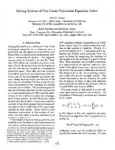


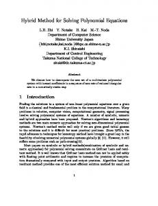


![FREE [P.D.F] Solving Systems of Polynomial Equations (CBMS ...](https://m.moam.info/img/260x300/free-pdf-solving-systems-of-polynomial-equations-c_6478412c097c474e708c9b86.jpg)


