Algorithms of Confidence Intervals of WG Distribution Based on ...

Journal of Computer and Communications, 2017, 5, 101-116 http://www.scirp.org/journal/jcc ISSN Online: 2327-5227 ISSN Print: 2327-5219

Algorithms of Confidence Intervals of WG Distribution Based on Progressive Type-II Censoring Samples Mohamed A. El-Sayed1,2, Fathy H. Riad3,4, M. A. Elsafty5, Yarub A. Estaitia2 Department of Mathematics, Faculty of Science, Fayoum University, Fayoum, Egypt Department of Computer Science, College of Computers and IT, Taif University, Taif, KSA 3 Department of Mathematics, Faculty of Science, Minia University, Minia, Egypt 4 Department of Mathematics, Faculty of Science, Aljouf University, Aljouf, KSA 5 Department of Mathematics and Statistics, Faculty of Science, Taif University, Taif, KSA 1 2

How to cite this paper: El-Sayed, M.A., Riad, F.H., Elsafty, M.A. and Estaitia, Y.A. (2017) Algorithms of Confidence Intervals of WG Distribution Based on Progressive Type-II Censoring Samples. Journal of Computer and Communications, 5, 101116. https://doi.org/10.4236/jcc.2017.57011 Received: March 1, 2017 Accepted: May 20, 2017 Published: May 23, 2017 Copyright © 2017 by authors and Scientific Research Publishing Inc. This work is licensed under the Creative Commons Attribution International License (CC BY 4.0). http://creativecommons.org/licenses/by/4.0/ Open Access

Abstract The purpose of this article offers different algorithms of Weibull Geometric (WG) distribution estimation depending on the progressive Type II censoring samples plan, spatially the joint confidence intervals for the parameters. The approximate joint confidence intervals for the parameters, the approximate confidence regions and percentile bootstrap intervals of confidence are discussed, and several Markov chain Monte Carlo (MCMC) techniques are also presented. The parts of mean square error (MSEs) and credible intervals lengths, the estimators of Bayes depend on non-informative implement more effective than the maximum likelihood estimates (MLEs) and bootstrap. Comparing the models, the MSEs, average confidence interval lengths of the MLEs, and Bayes estimators for parameters are less significant for censored models.

Keywords Algorithms, Simulations, Point Estimation, Confidence Intervals, Bootstrap, Approximate Bayes Estimators, MCMC, MLEs

1. Introduction The statistical distributions have a very important location of computer branches because of the great number of their particular applications. Being applied to images using Weibull distribution, the structured masks yield good results for the diagnosis of the early Alzheimer’s disease [1]. The paper [2] explores the relationship between the visible content and the real image statistics sampled by DOI: 10.4236/jcc.2017.57011 May 23, 2017

M. A. El-Sayed et al.

the integrated Weibull distribution. It presents a strong relationship between the brain and the parameters’ values using brain images. Moreover, the study discusses a simulated model of parameters estimated from the producer of EEG responses [3]. The Weibull distributions display significant statistics—because of their large number of particular features, and practitioners—due to their efficiency to suit data from several scopes, beginning with real data in life, to observation made in economics, weather data, acceptance sampling, hydrology, biology etc. [4]. The article deals with the Weibull-geometric (WG) distribution. The Weibull-geometric (WG), Exponential-Poisson (EP), Weibull-Power-Series (WPS), Complementary-Exponential-geometric (CEG), Exponential-Geometric (EG), Generalized-Exponential-Power-Series (GEPS), Exponential Weibull-Poisson (EWP), and Generalized-Inverse-Weibull-Poisson (GIWP) distributions are introduced and presented by Adamidis and Loukas [5], Kus [6], Chahkandi and Ganjali [7], Tahmasbi and Rezaei [8], Barreto [9], Morais and Barreto [10], Barreto and Cribari [11], Louzada et al. [12], and Cancho et al. [13]. Hamedani and Ahsanullah [14] studied and discussed many properties of WG, such as moments, hazard functions, and functions of order statistics. Barreto-Souza [9] suggested and studied the WG distribution. The modified Weibull geometric distribution introduced by composing the modified Weibull and geometric distributions and studied as class of lifetime distributions [15]. MohieEl-Din et al. [16] [17] and Elhag et al. [18] studied the confidence intervals for parameters of inverse Weibull distribution based on MLE and bootstrap. The paper is organized as follows: the probability density function and cumulative functions of the WG distribution are presented in Section 2. Section 3 provides Markov chain Monte Carlo’s algorithms. The maximum likelihood estimates of the parameters of the WG distribution, the point and interval estimates of the parameters, as well as the approximate joint confidence region are studied in Section 4. The parametric bootstrap confidence intervals of parameters are discussed in Section 5. Bayes estimation of the model parameters and Gibbs sampling algorithm are provided in Section 6. Data analysis and Monte Carlo simulation results are presented in Section 7. Section 8 concludes the paper.

2. WG Distributions It is assumed that there are n groups, independent and separated. Each group contains k items that are put in a lifetime test. Consider that the progressive

censored scheme R = { R1 , R2 , , Rm } such that: R1 represents a set of groups isolated and deleted from the current test, randomly, when the first failure X 1;Rm, n , k takes place. Similarly, R2 represents a combination of groups and the

group that the second failure is observed is deleted from the current test as soon as the second failure X 2;Rm, n , k occurs randomly. In final Rm , groups are randomly deleted from the current test when there is an m-th failure X mR;m,n ,k . Therefore, x1;Rm, n ,k < x2;R m, n ,k <  < xmR; m, n ,k , are known as progressively 1-failure censoring order statistics, where m is the number of the 1-failures 1 < m ≤ n . 102

M. A. El-Sayed et al.

The relation of the distribution function F ( x ) and probability density func-

tion f ( x ) are founded in the function of joint probability density for

X 1;Rm,n ,k , X 2;Rm,n ,k , , X mR;m,n ,k . The failure times of the k × n items from a conti-

nuous population are defined by: (see Balakrishnan and Sandhu [19])

(

)

f1, 2,, m x1;Rm, n ,k , x2;R m, n ,k , , xmR; m, n ,k m

(

)

(

)

= κ k m ∏ f xiR; m, n ,k 1 − F xiR; m, n ,k  i =1

k ( Ri +1)−1

(1)

,

0 < x1;Rm, n ,k < x2;R m, n ,k <  < xmR; m, n ,k < ∞, and

κ = n ( n − R1 − 1)( n − R1 − R2 − 2 ) ( n − R1 − R2 −  − Rm−1 − m − 1) .

(2)

There are special cases of the progressive first-failure censoring scheme of Equation (1) as follows:

1) When R = {0, 0, , 0} , the first-failure censoring scheme is obtained. 2) When k = 1 , the censoring order statistics of progressive Type II is found.

3) When R = {0, 0, , 0} and k = 1 , sampling case in the complete form is obtained. Generally, the progressively first-failure censoring order statistics X 1;Rm, n , k , X 2;Rm, n , k , , X mR; m, n , k can be represented as a censoring order statistics of

progressive Type II from the size of a population with function of distribution

1 − (1 − F ( x ) ) . Hence, the results of progressive type II can be expanded to k

progressive first-failure censoring order statistic easily. The testing time in the progressive first-failure-censoring plan is reduced with n × k items, which contains only m failures. The probability density function (pdf) of the WG distribution is represented by the following equation:

αβ (1 − p )( β x ) f ( x) =

α −1

e

α

−( β x )

(

1 − pe

α

−( β x )

), 2

x > 0,

(3)

and the cumulative distribution function (cdf) of the WG distribution is shown by:

(

α

F ( x) = 1− e ( ) − βx

) (1 − pe ) , α

−( β x )

x ≥ 0,

(4)

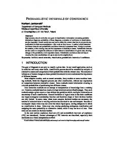
where α > 0; β > 0 and p ( 0 < p < 1) are parameters. The parameters α and β stand for the shape and scale while p stands for the mixing parameters, respectively. The WG distribution in Equation (3) produces some special models as follows: 1) Weibull distribution, when p = 0 . 2) WG distribution tends to a distribution that is degenerated in zero, when p →1. Hence, the parameter p can be explained as a focus parameter or concentration parameter. Figure 1 and Figure 2 show the density and cumulative plots 103

M. A. El-Sayed et al.

Figure 1. Shows Weibull-geometric density functions.

Figure 2. Displays Weibull-geometric cumulative functions.

respectively, with β = 0.9 and α = 5 for the various rates of p. The EG distribution related to two-parameter with decreasing failure rate is introduced by Adamidis and Loukas [5]. When α = 1 and 0 < p < 1 , the exponential geome-

tric (EG) distribution is obtained, and at α = 1 for any p < 1 the EEG distri-

bution is achieved. Therefore, the EEG distribution expands the EG distribution. The Weibull W (α , β ) distribution is obtained when p goes to zero. Figure 1 plots the WG density for some values of the vector ϕ = ( β , α ) when p =−2, −0.5, 0, 0.5, 0.9 . For all values of parameters, the density tends to zero as 104

M. A. El-Sayed et al.

x → ∞ . The density functions of WG are shown. It is noted that the WG density

is strictly decreasing when −1 ≤ p < 1 and α ≤ 1 , and is multimodal when −1 ≤ p < 1 and α > 1 . The form x0 = β −1u1 α is obtained when solution is arrived of the following nonlinear formulation: u + p −1eu ( u − 1 + 1 α ) =−1 + 1 α

(5)

The WG density can be unimodal when p < −1 . For instance, when p < −1 and α = 1 , the EEG distribution is unimodal. The hazard and survival functions of X are: h (t ) = αβ ( p − 1)( β t )

α −1

( pe

α −1

−( β t )

)

−1

(6)

)

(7)

and

(

S ( t ) =−1 + e

α

−( β t )

) ( pe

−1

α −1

−( β t )

−1 ,

3. Markov Chain Monte Carlo Algorithms Markov chain Monte Carlo (MCMC) technique has spread widely for Bayesian calculation in compound statistical modeling. In general, it gives a beneficial application for real statistical modeling (Gilks et al. [20]; Gamerman, [21]). Markov Chain is a randomly determined and stochastic process, having a random probability distribution or pattern that may be resolved statistically in that future cases are independent of previous cases specified the current case. Monte Carlo chain is an emulation and simulation, therefore; it used to solve integrals to some extent rather than analyze performance, a procedure named integration of Monte Carlo. In this way, interested quantities of a distribution can be picked from emulated draws and charts from the distribution. Bayesian test needs integration over probably high-dimension of probability distributions to produce predictions or to yield inference and deduction about parameters of model. Basically, Monte Carlo integration is utilized with chains of Markov in MCMC techniques. The patterns of integration draw from the desired distribution, and then form pattern rates to sacrificial expectations (see Geman [22]; Metropolis et al. [23]; and Hastings [24]).

3.1. MH Procedure The Metropolis-Hastings (MH) procedure is employed by Metropolis et al. [23]. It is assumed that the main target here is to design samples from the distribution f (τ | x ) = ℘(τ ) , where  is the normal fixed value which may be hard to

calculate or found. MH procedure gives a method of sampling from f (τ | x )

(

without the need to inform  . Suppose that  τ ( b ) | τ ( a )

)

is an optional transi-

tion kernel, where the probability of jumping, or moving, from existing case

τ ( a ) to τ (b ) , known as the suggestion or proposal distribution. The MH Algorithm generates values sequence τ (1) ,τ ( 2 ) , form a Markov chain with stable distribution given by f (τ | x ) . 105

M. A. El-Sayed et al.

Metropolis-Hastings Procedure

(

)

0 1) Select optional beginning value τ ( ) for which f τ ( 0 ) | x > 0 .

2) At time t sample candidate, points to or suggests that τ ∗ from

(

 τ ∗ |τ (

t −1)

) , the proposal distribution.

3) The approval probability is computed by:

(



)

χ τ ( t −1) ,τ ∗ = min 1,  

) (

(

f τ∗ | x  τ(

(

f τ(

t −1)

t −1)

|τ ∗

) (

| x  τ ∗ |τ (

)

t −1)

)

 .  

(8)

4) Produce W ∼ W ( 0,1) .

(

)

5) If W ≤ χ τ ( t −1) ,τ ∗ , the suggestion is accepted and put τ ( ) = τ ∗ , else refuse t

t t −1 the suggestion and put τ ( ) = τ ( ) 6) Repeat steps 2 - 5.

When the proposal distribution is symmetric, so  (τ | η ) =  (η | τ ) for all

(

) (

)

possible η and τ then, in particular, the result is  τ ( t −1) | τ ∗ =  τ ∗ | τ ( t −1) , so that the acceptance probability (5) is given by

(

)



(

)

 . t −1 f τ( ) | x   f τ∗ | x

χ τ ( t −1) ,τ ∗ = min 1,

(

 

(9)

)

3.2. GS Procedure Gibbs’ sampler (GS) procedure is a straightforward branch of MCMC algorithms. This procedure was implemented by Geman [22]. The significance of Gibbs’ procedure for area of issues in Bayesian analysis is explained by Gelfand and Smith [25]. The complete conditional distribution forms the transition kernel, so Gibbs sampler procedure is a MCMC planner. Gibbs sampling Procedure

(

)

1) Select optional beginning value τ ( 0 ) = τ 1( 0 ) , ,τ d( 0 )

( 3) By using conditional distribution ℘(τ 4) By using conditional distribution ℘(τ

( t −1)

2) By using conditional distribution ℘ τ 1 | τ 2 2 d

( t −1)

,τ 3

( )

for which ℘ τ ( 0 ) > 0. ( t −1)

, ,τ d

) , acquire

τ 1( t ) .

) , acquire τ ( ) . | τ ( ) ,τ ( ) ,τ ( ) , ,τ ( ) ) , acquire τ ( ) .

| τ 1( ) ,τ 3( t

1

t

t −1)

t 2

, ,τ 1( 3

t

t −1)

t d −1

t 2

t d

(5) Repeat steps 2 - 4.

The three unknown parameters of WG distribution will be studied through the various algorithms of estimation based on progressive Type-II censoring. The MCMC procedures are used with Bayesian technique to produce from the posterior distributions. 106

M. A. El-Sayed et al.

4. MLE of WG Distribution This section determines the maximum likelihood estimates (MLEs) of the WG R distribution parameters. Let’s assume that = X i X= 1, 2, , m are the i; m, n , i

progressive first-failure censoring order statistics from a WG distribution, with censoring plane R. Using Equations (1)-(3), the function of likelihood is shown by: m m   α n L (α , β , = p | x ) κα m β α m (1 − p ) × exp  (α − 1) ∑ log xi − ∑ ( β xi ) ( Ri + 1)  =i 1 =i 1  (10) m −( Ri + 2 ) α × ∏ 1 − p exp − ( β xi )    i =1

(

)

where κ is given in (2). The logarithm of the function of likelihood may be obtained as follow: l (α , β , p | x ) = m log α + mα log β + n log (1 − p ) m

m

+ (α − 1) ∑ log xi − ∑ ( β xi )

( Ri + 1)

α

=i 1 =i 1

(

m

(

− ∑ ( Ri + 2 ) log 1 − p exp − ( β xi ) i =1

Compute the derivatives

α

(11)

)) .

∂l ∂l ∂l , and , then put each equation equal ∂α ∂β pα

to zero, the likelihood equations can be obtained in the following: m m ∂l (α , β , p | x ) m α =+ m log β + ∑ log xi − ∑ ( Ri + 1)( β xi ) log ( β xi ) α ∂α =i 1 =i 1 m

− p∑

( Ri + 2 )( β xi )

α

(

1 − p exp − ( β xi )

i =1

α

m ∂l (α , β , p | x ) mα α −1 = − α ∑ ( Ri + 1) xi ( β xi ) ∂β β i =1 m

− pα ∑ i =1

( )

log ( β xi ) exp − ( β xi )

( Ri + 2 ) xi ( β xi )

α −1

(

(

exp − ( β xi )

α

1 − p exp − ( β xi )

α

and

α

(

)

m ( Ri + 2 ) exp − ( β xi ) ∂l (α , β , p | x ) −n = +∑ 1 − p i =1 1 − p exp − ( β x )α ∂p i

(

α

)

(12) )= 0,

(13) )= 0

)= (14) 0,

The analytical solution of αˆ , βˆ and pˆ in Equations (12)-(14) is very difficult. Hence, some numerical techniques like Newton’s method may be used. From the function of log-likelihood in (11), the Fisher information matrix

I (α , β , p ) is obtained by taking expectation of minus Equations (12)-(14). Under some mild regularity conditions, αˆ , βˆ , pˆ are approximately normal biva-

ly, in practice,

(

)

(α , β , p ) and covariance matrix I −1 (α , β , p ) . CommonI −1 (α , β , p ) is estimated by I −1 (αˆ , βˆ , pˆ ) . This procedure is

riate with the means

simpler and valid to employ the approximation.

107

M. A. El-Sayed et al.

(αˆ , βˆ , pˆ ) → N ((α , β , p ) , I (αˆ , βˆ , pˆ )) , −1 0

(15)

where I 0 (α , β , p ) is observed as information matrix.

I 0−1

(

 ∂ 2l ( x;α , β , p ) − ∂α 2   ∂ 2l ( x;α , β , p ) − αˆ , βˆ , pˆ = ∂β∂α   2  − ∂ l ( x;α , β , p )  ∂p∂α 

)

(

−

∂ 2l ( x;α , β , p ) ∂α∂β

−

∂ 2l ( x;α , β , p ) ∂β 2

−

∂ 2l ( x;α , β , p ) ∂p∂β

 var (αˆ ) cov αˆ , βˆ  var βˆ = cov βˆ , αˆ  ˆ  cov ( pˆ , αˆ ) cov pˆ , β

(

)

(

( )

) )

−1

∂ 2l ( x;α , β , p )   ∂α∂p  ∂ 2l ( x;α , β , p )   − ∂β∂p   2 ∂ l ( x;α , β , p )  − (16)  ˆ ∂p 2  (αˆ , β , pˆ ) −

cov (αˆ , pˆ )   cov βˆ , pˆ  .  var ( pˆ )  

(

)

Confidence intervals can be calculated approximately for α , β and p to be

bivariate normal distributed with the means (α , β , p ) and covariance matrix I 0−1 αˆ , βˆ , pˆ . Hence, the 100 (1 − α ) % confidence intervals approximately for α , β and p are

(

)

αˆ ± zα v11 , βˆ ± zα v22 and pˆ ± zα v33 2

2

2

(17)

respectively, where the values v11 , v22 and v33 are on the major diagonal of the covariance matrix I 0−1 αˆ , βˆ , pˆ and zα is the percentage of the standard 2 α . normal distribution with right-tail probability 2

)

(

5. Intervals of Bootstrap Confidence The bootstrap technique is used for resampling in statistical inference cases. It is usually utilized to evaluate confidence regions and it can be applied to evaluate bias and variance of a calibrator or estimator assumption tests. Additional scanning of the parametric and nonparametric bootstrap technique is applied, see Davison and Hinkley [26], and Elhag et al. [27]. The parametric bootstrap technique of the two confidence intervals is suggested. The algorithm for evaluating the confidence intervals of parameters uses both Efron and Tibshirani procedures [28], and bootstrap-t Hall procedure [20]. The Bootstrap sampling algorithm for estimating the confidence intervals of parameters is illustrated below. Bootstrap Sampling Algorithm 1) Using the normal progressively Type-II samples, x =

( x1 < x2 <  < xm ) ,

obtain αˆ , βˆ , and pˆ , j = 1, 2, 3 . 2) Using the values of n and m ( 1 < m ≤ n ) with the same values of R, = 2, , m ) , j 1, 2, 3 , generate random sample of sizes m from WG distri( i 1,= bution, x* =

(x

* 1

< x2* <  < xm*

krishnan and Sandhu [5]. 108

)

based on the procedure introduced in Bala-

M. A. El-Sayed et al. Continued

3) Use x* as in step 1 to calculate the bootstrap sample estimates of αˆ , βˆ and pˆ indicated as αˆ * , βˆ * and pˆ * . 4) By repeating the steps 2 and 3 N times, where N is the number of various bootstrap samples, put N = 1000. 5) Sort all values of αˆ * , βˆ * and pˆ * in an ascending order to get bootstrap sample

(ϕ [ ] , ϕ [ ] , , ϕ [ ] ) , k = 1, 2, 3 *1 k

*N k

*2 k

(

)

∗ ∗ , ϕ2* β= , ϕ3* p∗ . ϕ1* αˆ= where=

(

)

Percentile bootstrap confidence interval: Assume that G= ( y ) P ϕˆ ∗j ≤ y is the cumulative distribution function of ϕˆ ∗j . Determine ϕˆ ∗jboot = G −1 ( y ) for the given y. The bootstrap confidence interval approximately with 100 (1 − γ ) % of ϕˆ ∗j may be obtained as follows:

 ∗  γ  ∗  γ  ϕˆ jboot  2  , ϕˆ jboot 1 − 2   .     

(18)

∗1 ∗2 ∗N First, locate the sort statistics δ j [ ] < δ j [ ] <  < δ j [ ] , wherever

ϕˆ ∗j[i ] − ϕˆ j

δk[ ] = ∗i

, i 1,= 2, , N , j 1, 2, 3, = ∗i var ϕˆ j[ ]

( )

and= ϕˆ1 αˆ= , ϕˆ2 βˆ= , ϕˆ3 pˆ . Consider that H= ( y ) P δ ∗j < y

(

δ . If y is given, then ∗ j

)

(19)

is the cumulative distribution function of

ϕˆ jboot −= ϕˆ j + var (ϕˆ j ) H −1 ( y ) . t

(20)

6. Bayes Estimation of the Model Parameters In the consideration that each of the parameters α , β and p are unknown, it may be considered that the joint prior density is a product of gamma density of

α and β uniform prior of p, where

π= 1 (α ) π= 2 (β )

ba α a−1 exp ( −bα ) , α > 0, ( a, b > 0 ) , Γ (a)

(21)

dc β c−1 exp ( −d β ) , β > 0, ( c, d > 0 ) , Γ (c)

(22)

and

π3 ( p) = 1

(23)

By multiplying π 1 (α ) by π 2 ( β ) and π 3 ( p ) , we get the joint prior density of α , β and p computed by = π (α , β , p )

ba d c α a−1β c−1 exp ( − ( bα + d β ) ) , (α , β > 0 and 0 ≤ p ≤ 1) . (24) Γ (a) Γ (c)

Based on the prior of joint distribution of α , β and p the posterior of joint density function of α , β and p known as the data, indicated by π ∗ (α , β , p | x ) 109

M. A. El-Sayed et al.

can be expressed as follows:

π ∗ (α , β , p | x ) =

L (α , β , p | x ) × π (α , β , p ) ∞

∞

∞

∫0 ∫0 ∫0

L (α , β , p | x ) × π (α , β , p ) dα dβ dp

.

(25)

Hence, using squared error loss function (SEL) of any function ϕ (α , β , p ) , the Bayes estimate of α , β and p can be expressed as

ϕˆ (α , β , p ) = Eα , β , p|x (ϕ (α , β , p ) ) ∞

∞

∞

∫ ∫ ∫ ϕ (α , β , p ) L (α , β , p | x ) × π (α , β , p ) dα dβ dp = 0 0 0∞ ∞ ∞ ∫0 ∫0 ∫0 L (α , β , p | x ) × π (α , β , p ) dα dβ dp

(26)

In general, the value of two integrals specified by (26) cannot be acquired in a cleared and closed format. In this situation, the MCMC procedure is used to create patterns from the posterior distributions and; therefore, is calculated the

Bayes estimator of ϕ (α , β , p ) along with the function of SEL. A wide diversity of MCMC techniques is available and can be troublesome to select any of them. A significant type of MCMC technique is Gibbs samplers and widespread Metropolis within-Gibbs samplers. The MCMC procedure has the advantage over the MLE procedure that we can permanently gain an appropriate estimation of intervals of the parameters by building the probability intervals and using the experimental posterior distribution. This, sometimes, is not obtainable in MLE. The samples of MCMC can be utilized to fully brief the uncertainty of posterior about the parameters α , β and p , by using a kernel estimation of the posterior distribution.

The function of joint posterior density of α , β and p may be described as 

m

π ∗ (α , β , p | x ) ∝ α m+a−1β α m+c−1 (1 − p ) exp −bα − d β + α ∑ log xi n



i =1

(

)

α α −∑ ( Ri + 2 ) log 1 − p exp − ( β xi )  − ∑ ( Ri + 1)( β xi )  .   =i 1 =i 1  m

m

(27)

The conditional posterior PDF’s of α , β and p are shown as

 

m



 

i =1



π 1∗ (α | β , p, x ) ∝ α m+a−1 exp α  m log β − b + ∑ log xi 

(

m

−∑ ( R + 2 ) log 1 − p exp − ( β x 

)

α

) − ∑ ( R + 1)( β x ) m

α

i i =i 1 =i 1

i

i

(

 , 

)

 α π 2∗ ( β | α , p, x ) ∝ β α m+c−1 exp −d β − ∑ ( Ri + 2 ) log 1 − p exp − ( β xi )  m



i =1

m

−∑ ( Ri + 1)( β xi )

α

i =1



 , 

(28)

(29)

and

(

)

  α n π 3∗ ( p | α , β , x ) ∝ (1 − p ) exp −∑ ( Ri + 2 ) log 1 − p exp − ( β xi )   .   m



i =1

(30)

The Metropolis-Hastings procedure [23] with normal proposal distribution 110

M. A. El-Sayed et al.

under the Gibbs sampler algorithm is described as follows: Gibbs/Metropolis-Hastings Sampler Algorithm 0 1) Initialize I = 1 , α ( ) = αˆ and β ( 0 ) = βˆ . I 2) Based on Metropolis-Hastings, create α ( ) using (28) with the

(

N α(

I −1)

, σ1

)

proposal distribution, where σ 1 is from

variances-covariance matrix. 3) Based on Metropolis-Hastings, create β ( I ) using (29) with the

(

N β(

I −1)

,σ 2

)

proposal distribution, where σ 2 is from

variances-covariance matrix. 4) Based on Metropolis-Hastings, create p ( I ) using (30) with the

(

N p(

I −1)

,σ 3

)

proposal distribution, where σ 3 is from

variances-covariance matrix. 5) Calculate α ( I ) , β ( I ) and p ( I ) . 6) Put I= I + 1 . 7) Repeat steps (2 - 5) N times. 8) We get the point estimation by Bayes MCMC of ϕl = ( ϕ1 α= , ϕ2 β and

ϕ3 = p ) as E (ϕ l | x ) =

N 1 ϕl(i ) , ∑ N − M =i M +1

(31)

where M is the number of iterations (burn-in period) before the stationary distribution is accomplished and posterior variance of ϕl becomes

= Vˆ (ϕl | x )

(

)

N 2 1 ϕl(i ) − Eˆ (ϕl | x ) , ∑ N − M =i M +1

(32)

9) The quintiles of the pattern are picked as the endpoints of the interval to calculate the reliable intervals of ϕl . Sort ϕl( M +1) , ϕl( M + 2 ) , , ϕl( N ) as ϕl (1) , ϕl ( 2 ) , , ϕl ( N −M ) . Hence, the symmetric credible interval with 100 (1 − γ ) % is

  ϕ  γ  ϕ ,  l  2 ( N −M )  l  1− γ2 ( N −M )      

(33)

7. Illustrative Example and Simulation Studies To explain the procedures evolved of estimation in this paper, gamma distribu= b 1 ) is used and produce sample of tion for given hybrid parameters= ( a 1.5, 1 10 space 10, randomly (21), the average of the sample α ≅ ∑α i , is computed 10 i =1 and supposed as the real population rate of α = 1.5 . So that they are obtained to b verify E (α = ) ≅ α with the past parameters is nearly the average of gamma a distribution. Similarly, when the valued c = 2 and d = 1 are given, create 111

M. A. El-Sayed et al.

π 2 ( β ) based on the last β = 2 , from gamma distribution (22). The previously

d ≅ β , are nearly the average of gamma c distribution. A progressive Type II samples are created by employing the proce-

parameters selected to verify E ( β = )

dures of Balakrishnan and Sandhu [19] from WG distribution with the available data: 0.0409, 0.0552, 0.0561, 0.0726, 0.0776, 0.0840, 0.0906, 0.1108, 0.1291, 0.1502, 0.1513, 0.1540, 0.1624, 0.1691, 0.1930, 0.2175, 0.2188, 0.2700, 0.2709, 0.2994, 0.3219, 0.3342, 0.4065, 0.4396, 0.5385, and under the parameters; ( α = 1.5 , p = 0.6 , β = 2 , m= n= 50 and R = {2, 0, 2, 0,1, 0, 2, 0, 0, 3, 0, 0, 2, 0, 2, 0,1, 0, 3, 0, 3, 0, 2, 0, 2} ).

The approximate bootstrap, Bayes estimates and MLEs are calculated of α , β , and p under these data utilizing MCMC algorithm outputs are explained in Table 1 and Table 2. Table 2 yield the 95%, approximate confidence intervals of two bootstrap, approximate credible and MLE under the MCMC samples. Studies of simulation have been executed employing Mathematica ver. 9.0 for explaining the theoretic outcomes of estimates issue. The accomplishment of the performing estimators of the parameters has been supposed in valued of their mean square error (MSE) and average (AVG), where

= ϕˆk

1 M

M

(ϕ1 ∑ ϕˆk( ) , = i

i =1

α= , ϕ2 β= , ϕ3 p ) ,

(34)

and

= MSE

1 M

∑ (ϕˆk( ) − ϕk ) M

i

2

.

(35)

i =1

In studies of simulation, the researchers assume that the population parameter rates= = β 1.5, = p 0.1) , various sample values n, different effected sam(α 0.5, ple size m and different censored scheme R . For computing Bayes estimators, without loss of generality using non-informative priors, ( a = 0.0001 , b = 0.0001 , c = 0.0001 , d = 0.0001 ). Under function of squared error loss, the researchers calculate the Bayes estimations. The estimations of Bayes and 95% credible intervals using 11,000 sets of MCMC are also calculated. The mean Bayes estimaTable 1. Show the parameters estimation of WG distribution. Procedure

α = 1.5

β = 2.0

p = 0.6

(.)ML

1.6178

1.9614

0.4566

(.)Boot

1.8122

2.2451

0.7724

(.)MCMC

1.6299

1.9787

0.4727

Table 2. Show the CIs using Bootstrap, Bootstrap-t and MLE according to 500 times.

112

Procedure

α = 1.5

β = 2.0

p = 0.6

(.)ML

(1.1424, 2.0931)

(1.3282, 2.5946)

(0.4654, 0.9210)

(.)Boot

(1.0004, 2.3599)

(1.1012, 2.5840)

(0.4655, 0.8821)

(.)Boot-t

(1.1235, 2.0147)

(0.8561, 2.6523)

(0.1361, 0.8111)

(.)MCMC

(1.1444, 1.9440)

(0.9569, 2.5709)

(0.0361, 0.7768)

M. A. El-Sayed et al.

tions, MSEs, coverage percentages, and average lengths of confidence interval based on 500 times are reported. Comparatively, the MLEs with the 95% confidence intervals are calculated based on the observation of Fisher information matrix and two bootstrap confidences. Table 3 and Table 4 report the outputs based on MLEs and the Bayes estimations utilizing both the Gibbs sampling algorithm and MH algorithm: 1) From Table 3 and Table 4, in parts of MSEs and credible intervals lengths, the estimators of Bayes depend on non-informative implement more effective than the MLEs and bootstrap. 2) From Table 3 and Table 4, comparing the models, the MSEs, average confidence interval lengths of the MLEs, and Bayes estimators for parameters are less significant for censored models

( n − m, 0, ⋅ ⋅ ⋅, 0 ) .

3) The MSE and average confidence interval lengths nearly reduce the estimators in whole situations when the performance sample rate n m raises.

8. Conclusion Several algorithms of estimation of WG distribution, based on the progressive Type II censored sampling plan, are discussed. The joint confidence intervals for the parameters are also studied. The approximate confidence regions, percentile bootstrap confidence intervals, as well as approximate joint confidence region Table 3. Show the various estimators average values and the identical MSEs when = α 0.5, = β 1.5 and p = 0.1 . m (scheme)

Bayes ( MCMC )

Boot

MLE α

β

p

α

β

p

α

β

p

0.6245

1.6664

0.1021

0.7241

1.4217

0.1539

0.5241

1.4399

0.1597

0.1234

0.4736

0.0664

0.2235

0.4840

0.1021

0.1200

0.1914

0.1056

0.6754

1.6828

0.1016

0.6788

1.4027

0.1482

0.5751

1.4194

0.1533

0.2101

0.5398

0.0614

0.2479

0.5438

0.0906

0.1101

0.4530

0.0936

0.5364

1.7667

0.1001

0.5388

1.3614

0.1554

0.5064

1.3977

0.1621

0.2351

0.7337

0.0707

0.3331

0.8748

0.1069

0.1111

0.5925

0.1105

0.6200

1.6165

0.1023

0.7070

1.4327

0.1432

0.5205

1.4424

0.1471

0.1088

0.3890

0.0623

0.1282

0.3347

0.0874

0.0988

0.3389

0.0596

0.6151 20 (1, 0, ···, 1, 0) 0.1901

1.6173

0.1024

0.6999

1.4234

0.1404

0.5151

1.4322

0.1439

0.4028

0.057

0.2220

0.4500

0.0793

0.1102

0.3543

0.0511

0.6164

1.6782

0.0968

0.7162

1.4204

0.1400

0.5146

1.4375

0.1443

0.2225

0.5091

0.0577

0.2335

0.6194

0.0813

0.1325

0.4272

0.0537

0.5777

1.7881

0.0974

0.7357

1.4828

0.1297

0.5577

1.4934

0.1320

0.1100

0.7534

0.054

0.2102

0.7296

0.0707

0.0985

0.6377

0.0518

0.6360

1.9606

0.094

0.5399

1.5464

0.1233

0.6355

1.5575

0.1254

0.1840

1.0418

0.0447

0.1990

0.9999

0.0570

0.1000

0.8539

0.0480

0.6321

2.1049

0.0950

0.6355

1.4381

0.1320

0.6333

1.4661

0.1351

0.2114

1.5074

0.0548

0.2554

1.5381

0.0741

0.2000

1.2615

0.0758

15 (15, 140)

15 (151)

15 (140, 15)

20 (10, 190)

20 (190, 10)

30 (30, 290)

30 (130)

30 (290, 30)

113

M. A. El-Sayed et al. Table 4. Show the coverage percentages and average confidence interval, when = = α 0.5, β 1.5 and p = 0.1 . m (scheme) 15 (15, 140)

15 (151)

MLE

Bayes ( MCMC )

Boot

α

β

p

α

β

p

α

β

p

0.90

0.923

0.87

0.892

0.933

0.86

0.9021

0.916

0.936

0.7502

1.6373

0.2507

0.9840

1.8201

0.3503

0.7001

1.5616

0.3504

0.901

0.923

0.874

0.9011

0.963

0.894

0.910

0.952

0.952

0.8821

1.9465

0.2358

0.9991

2.012

0.4458

0.8111

1.8784

0.3231

0.880

0.908

0.886

0.874

0.918

0.896

0.891

0.933

0.939

0.9921

2.5915

0.3571

1.001

2.5313

0.4574

0.8821

2.4269

0.3695

0.911

0.945

0.883

0.933

0.947

0.890

0.924

0.943

0.936

0.7001

1.4041

0.2222

0.8801

1.3331

0.3332

0.3001

1.3522

0.2932

0.905 20 (1, 0, ···, 1, 0) 0.7721

0.962

0.895

0.915

0.920

0.905

0.932

0.958

0.943

1.5183

0.2133

0.8723

1.6683

0.2442

0.7028

1.4749

0.2778

0.891

0.963

0.857

0.901

0.980

0.889

0.901

0.968

0.965

0.9823

1.9051

0.2237

0.9977

1.9352

0.2299

0.7023

1.8133

0.302

15 (140, 15)

20 (10, 190)

20 (190, 10) 30 (30, 290) 30 (130) 30 (290, 30)

0.933

0.943

0.855

0.906

0.955

0.921

0.935

0.945

0.946

0.6002

2.4938

0.1935

0.6880

2.8888

0.1991

0.5001

1.4563

0.2011

0.925

0.946

0.873

0.933

0.920

0.913

0.965

0.959

0.975

0.7522

3.4213

0.13

0.7588

1.4211

0.118

0.6122

1.4142

0.223

0.901

0.945

0.855

0.921

0.944

0.952

0.933

0.956

0.956

0.7923

1.1995

0.1061

0.8925

1.1997

0.1880

0.6982

1.0515

0.260

for the parameters are expanded and developed. Some numerical examples with actual data set and simulated data are used to compare the proposed joint confidence regions. The parts of MSEs and credible intervals lengths, the estimators of Bayes depend on non-informative implement more effective than the MLEs and bootstrap. Comparing the models, the MSEs, average confidence interval lengths of the MLEs, and Bayes estimators for parameters are less significant for censored models.

References

114

[1]

Al-jibory, W.K.S. and EI-Zaart, A. (2013) Edge Detection for Diagnosis Early Alzheimer’s Disease by Using Weibull Distribution. 25th International Conference on Microelectronics (ICM), Beirut, 15-18 December 2013.

[2]

Scholte, H.S. and Ghebreab, S. (2009) Lourens Waldorp. In: Arnold, W.M.S. and Victor, A.F.L., Eds., Brain Responses Strongly Correlate with Weibull Image Statistics When Processing Natural Images, Vol. 9, 29. https://doi.org/10.1167/9.4.29

[3]

El-Sayed, M.A., Abd-Elmougod, G.A. and Abdel-Khalek, S. (2013) Bayesian and Non-Bayesian Estimation of Topp-Leone Distribution Based Lower Record Values. Far East Journal of Theoretical Statistics, 45, 133-145.

[4]

Afify, A.Z., Nofal, Z.M. and Butt, N.S. (2014) Transmuted Complementary Weibull Geometric Distribution. Pakistan Journal of Statistics and Operation Research, 10, No. 4.

[5]

Adamidis, K. and Loukas, S. (1998) A Lifetime Distribution with Decreasing Failure

M. A. El-Sayed et al. Rate. Statistics and Probability Letters, 39, 35-42. [6]

Kus, C. (2007) A New Lifetime Distribution. Computational Statistics & Data Analysis, 51, 4497-4509.

[7]

Chahkandi, M. and Ganjali, M. (2009) On Some Lifetime Distributions with Decreasing Failure Rate. Computational Statistics and Data Analysis, 53, 4433-4440.

[8]

Tahmasbi, R. and Rezaei, S. (2008) A Two-Parameter Lifetime Distribution with Decreasing Failure Rate. Computational Statistics and Data Analysis, 52, 3889-3901.

[9]

Barreto-Souza, W. (2011) The Weibull-Geometric Distribution. Journal of Statistical Computation and Simulation, 81, 645-657. https://doi.org/10.1080/00949650903436554

[10] Morais, A.L. and Barreto-Souza, W. (2011) A Compound Class of Weibull and Power Series Distributions. Computational Statistics and Data Analysis, 55, 14101425. [11] Barreto-Souza, W. and Cribari-Neto, F. (2009) A Generalization of the Exponential-Poisson Distribution. Statistics and Probability Letters, 79, 2493-2500. [12] Louzada, F., Roman, M. and Cancho, V.G. (2011) The Complementary Exponential Geometric Distribution: Model, Properties, and Comparison with Its Counterpart. Computational Statistics and Data Analysis, 55, 2516-2524. [13] Cancho, V.G., Louzada-Neto, F. and Barriga, G.D.C. (2011) The Poisson-Exponential Lifetime Distribution. Computational Statistics and Data Analysis, 55, 677686. [14] Hamedani, G.G. and Ahsanullah, M. (2011) Characterizations of Weibull Geometric Distribution. Journal of Statistical Theory and Applications, 10, 581-590. [15] Wang, M. and Elbatal, I. (2015) The Modified Weibull Geometric Distribution. METRON, 73, 303-315. [16] El-Din, M.M., Riad, F.H. and El-Sayed, M.A. (2014) Confidence Intervals for Parameters of IWD Based on MLE and Bootstrap. Journal of Statistics Applications & Probability, 3, 1-7. [17] El-Din, M.M., Riad, F.H. and El-Sayed, M.A. (2014) Statistical Inference and Prediction for the Inverse Weibull Distribution Based on Record Data. International Journal of Advanced Statistics and Probability, 3, 171-177. [18] Elhag, A., Ibrahim, O.I.O. and, El-Sayed, M.A. (2014) Some Features of Joint Confidence Regions for the Parameters of the Inverse Weibull Distribution. Mathematical Theory and Modeling Journal, 4, 118-124. [19] Balakrishnan, N. and Sandhu, R.A. (1995) A Simple Simulation Algorithm for Generating Progressively Type-II Censored Samples. The American Statistician, 49, 229-230. [20] Gilks, W.R., Richardson, S. and Spiegelhalter, D.J. (1996) Markov Chain Monte Carlo in Practices. Chapman and Hall, London. [21] Gamerman, D. (1997) Markov Chain Monte Carlo: Stochastic Simulation for Bayesian Inference. Chapman and Hall, London. [22] Geman, S. and Geman, D. (1984) Stochastic Relaxation, Gibbs Distributions, and the Bayesian Restoration of Images. IEEE Transactions on Pattern Analysis and Mathematical Intelligence, 6, 721-741. https://doi.org/10.1109/TPAMI.1984.4767596 [23] Metropolis, N., Rosenbluth, A.W., Rosenbluth, M.N., Teller, A.H. and Teller, E. (1953) Equations of State Calculations by Fast Computing Machines. Journal Chemical Physics, 21, 1087-1091. https://doi.org/10.1063/1.1699114 115

M. A. El-Sayed et al. [24] Hastings, W.K. (1970) Monte Carlo Sampling Methods Using Markov Chains and Their Applications. Biometrika, 57, 97-109. https://doi.org/10.1093/biomet/57.1.97 [25] Gelfand, A.E. and Smith, A.F.M. (1990) Sampling Based Approach to Calculating Marginal Densities. Journal of the American Statistical Association, 85, 398-409. https://doi.org/10.1080/01621459.1990.10476213 [26] Davison, A.C. and Hinkley, D.V. (1997) Bootstrap Methods and Their Applications. 2nd Edition, Cambridge University Press, Cambridge. https://doi.org/10.1017/CBO9780511802843 [27] Elhag, A.A., Ibrahim, O.I., El-Sayed, M.A. and Abd-Elmougod, G.A. (2015) Estimations of Weibull-Geometric Distribution under Progressive Type II Censoring Samples. Open Journal of Statistics, 5, 721-729. https://doi.org/10.4236/ojs.2015.57072 [28] Efron, B. and Tibshirani, R.J. (1993) An Introduction to the Bootstrap. Chapman and Hall, New York. https://doi.org/10.1007/978-1-4899-4541-9

Submit or recommend next manuscript to SCIRP and we will provide best service for you: Accepting pre-submission inquiries through Email, Facebook, LinkedIn, Twitter, etc. A wide selection of journals (inclusive of 9 subjects, more than 200 journals) Providing 24-hour high-quality service User-friendly online submission system Fair and swift peer-review system Efficient typesetting and proofreading procedure Display of the result of downloads and visits, as well as the number of cited articles Maximum dissemination of your research work

Submit your manuscript at: http://papersubmission.scirp.org/ Or contact [email protected]

116