SENSITIVITY ANALYSIS OF CREEP & FATIGUE CRACK GROWTH IN HIGH ..... C* approach: in this case non-linear fracture mechanics based modelling is ...
Probabilistic Analysis of Crack Growth
OMMI (Vol.3, Issue 2) August 2004
www.ommi.co.uk
ALIAS-HIDA, A KNOWLEDGE-BASED SYSTEM FOR PROBABILISTIC & SENSITIVITY ANALYSIS OF CREEP & FATIGUE CRACK GROWTH IN HIGH TEMPERATURE COMPONENTS A Jovanovic, D Colantoni, D Balos & G Wagemann, MPA Stuttgart, Germany; N Le Mat Hamata, European Technology Development, UK; H Deschanels, Framatome ANP / Novatome, France
Abstract The paper presents results in the development of the Knowledge-Based System, called ALIASHIDA, developed within the framework of the HIDA Applicability Project for predicting the remaining life of high temperature components containing crack-like defects. In order to handle uncertainties and variations in critical inputs, the system, which was initially developed for the deterministic HIDA Defect Assessment Procedure, was extended to include methods to perform both sensitivity and probabilistic analyses. The ALIAS-HIDA was implemented within the ALIAS software (Advanced LIfe Assessment System of the Institute for Testing of Materials, MPA University of Stuttgart, Germany) and, within the HIDA Applicability project, extensive testing and application of this system were performed by the HIDA partners using the HIDA databank and HIDA test results. Examples of the application of the different options offered within ALIAS-HIDA (i.e. deterministic, sensitivity and probabilistic analyses) are presented and the prediction results show good correlation when compared to reference data.
1. Introduction The formulation and application of procedures [1]-[4] which deal with crack initiation and crack growth in components under creep/fatigue regime are promoted since the necessity to assure safety conditions of the plant and guarantee the extension of the component life beyond the original design lifetime is among the main intents of high temperature plant/component management. When defects are found during the in-service inspections, immediate repair or replacement of the damaged components might not always be needed with a consequent optimisation of the plant/component operation. Nowadays most of these crack assessment procedures normally used in high temperature plants’ service are deterministic thus requiring appropriate, preferably cast specific, data input to determine the crack behaviour and remaining life of components containing design allowable manufacturing or service induced defects. However, often it is not possible to have direct access to this specific data. As a result, the life assessment is not reliable and in most cases, it is based on the worst combination of input data resulting in a too conservative prediction, which does not take into account any optimisation of costs or improvement of plant efficiency.
Probabilistic Analysis of Crack Growth
OMMI (Vol.3, Issue 2) August 2004
2
Furthermore, the prediction of life expectancy of a cracked component is strongly influenced by a wide range of parameters (the geometry of the component and of the defect, available material properties including welds and HAZ data, operating conditions, methodologies employed to assess the crack behaviour), which generally exhibit significant uncertainties/ scatter. In particular, when assessing the crack growth in a cracked component, it is necessary to take into consideration: • The initial defect size, shape and location, which may be subject to measurement errors; • The component geometry, which can also not be accurately identified (e.g. imprecise measurements of the wall thickness); • The operating conditions (such as load, temperature, etc.), which may sustain variations with time; • The material properties, which may not be precise [5]. When dealing with uncertainties in the material properties, the most conservative values are frequently used in order to obtain a lower bound life assessment. However, the results produced following such an approach are over-conservative and the margin of conservatism cannot be estimated with sufficient precision. In addition, for a certain parameter, it is not always clear which bound leads to a conservative assessment. For example, a high strength material with low ductility will show a fast creep crack growth rate but a larger critical size under upper bound toughness, yield or rupture criteria. On the other hand, a low strength material with high ductility will have a low creep crack growth rate but a smaller critical crack size. Which of these behaviours will result in the shorter component life is not obvious. Therefore it is only with probabilistic techniques that the defect assessment procedures can lead to results, which reduce the degree of conservatism that is inherent when the crack development is estimated without taking uncertainties into consideration in an appropriate way. Thus all variations in the input parameters can be quantified and their effects can be correctly merged into a distribution of results, the most important output of such an approach being in fact the probability of failure as a function of the service time. Before performing such probabilistic analysis, it is essential to estimate the impact and significance that these uncertainties have on the component life prediction, and to identify those that only require a probabilistic evaluation. Hence it becomes of crucial importance to isolate through a sensitivity analysis the parameters that mostly affect the component in terms of remaining life, parameters that then will be considered as stochastic variables in the probabilistic analysis. Crack assessment procedures that can evaluate the probability of failure through probabilistic methods introduced into the operating service of industrial plants will provide direct benefits as they will increase the safety of the plant and improve the capability of extending the remaining life of components. In particular, they will enhance the decision making process, enabling the development of cost effective maintenance and plant rehabilitation strategies. In fact, substantial reductions in production costs can be achieved by reducing the frequency of unplanned outages, increasing the operating periods between scheduled inspections, improving plant availability and efficiency and avoiding costs associated with the replacement of expensive components.
Probabilistic Analysis of Crack Growth
OMMI (Vol.3, Issue 2) August 2004
3
2. Overview of the ALIAS-HIDA The ALIAS-HIDA is based on the KBS developed for the HIDA project (BRITE/EURAM project “HIDA”, BE 1702, [6] and [7]) to which new features have been added. Figure 1 to Figure 3 show the schematic flow charts associated with a typical deterministic, sensitivity and probabilistic analysis that can be performed using the current ALIAS-HIDA. As it can be seen from these figures, the accomplishment of each analysis is subdivided in the completion of specific steps, which comprise: • Setup • Input • Calculation of main parameters • Failure criteria check • Calculation of crack growth rates • Analysis: deterministic, sensitivity or probabilistic 2.1.
Setup
The first action that has to be completed when starting a new analysis is to specify its characteristics, which include setting: • Type of assessment: This can be either deterministic or probabilistic, i.e. whether uncertainties in the input parameters have to be considered. The result of a deterministic analysis will be the crack growth of the initial detected defect to failure, while the result of a probabilistic analysis will be the time to failure for a specified target probability of failure, and in general the probability of failure as a function of the service time; • Type of geometry: This includes the orientation and location of the defect, if applicable. The considered geometries [8] comprise specimens (e.g. compact tension specimen, single edge notched tension specimen) and components (straight pipes, elbows, T-pieces); • Type of regime: i.e. pure creep, pure fatigue or interaction of creep and fatigue; • Method used for the calculation of the stress intensity factor: different methods are available including national standards (e.g. British BS 7910 [1] and French RCC-MR [2]) or other sources (e.g. SINTAP); • Definition of stresses: The primary stresses can be calculated from the loading or can be directly input. When present, the secondary stresses can be represented as a distribution through the wall thickness described by a polynomial function, which coefficients σ is (i = 0 to 3) need to be input; this is the case for example of FE results of thermal stresses or measurements of residual stresses in weldments: 2
3
u u u σ sec ondary = σ 0s + σ 1s + σ 2s + σ 3s L L L The polynomial is expressed as a function of the reduced variable (u/L), where L is length of the smoothing range which can be restricted to the size of the defect improved accuracy (a ≤ L ≤ t, with a being the defect size and t the thickness of component) and u is the variable within this range 0 ≤ u ≤ L [2].
(1) the for the
Probabilistic Analysis of Crack Growth
2.2.
OMMI (Vol.3, Issue 2) August 2004
4
Input
After specifying the analysis in its general terms, the geometry of the component and of the defect, the properties of the material, the service conditions and the loading applied have to be numerically characterised. The geometry of the component and of the defect will require different inputs depending on the selected component. For example, for a straight pipe with circumferential semi-elliptical external defect, the depth and half-length of the defect, the wall thickness and the inner radius of the pipe have to be specified. The material properties comprise: • Fracture and tensile data. • Creep strain rate data: the creep behaviour that dominates the high temperature crack growth either can be only secondary (steady state) creep described by a power law in terms of the applied stress: n ε& sc = Asσ ref (2a) If the material exhibits an important primary creep stage that also affects the crack growth, this behaviour is then described by a power law in terms of the applied stress and time: n1 α ε& cp = A p σ ref t (2b) In this case the strain rate resulting from primary and secondary creep is given by: n1 α n ε& c = max ε& cp ; ε& sc = max A pσ ref t ; Asσ ref
(
)
(
)
(2c)
Creep rupture data: the time to rupture at the reference stress can be evaluated using a power law formulation: ν t r = B (σ ref ) (3a) or a log power law formulation: H t r = log −1 P(σ ref )(TK − G ) + F (3b) where: 2 3 4 P(σ ref ) = a + b(log σ ref ) + c(log σ ref ) + d (log σ ref ) + e(log σ ref ) (3c) Fatigue crack growth data: the fatigue crack growth can be described with the Paris law: da m m m (4a) = C∆K eff = Cq0 ∆K = Cq 0 [(1 − R) K I ] dN fat where ΔK is the stress intensity factor range, KI is the stress intensity factor and q0 is a parameter that takes into account the crack closure during the compressive loading of the applied cycle. It can be estimated using the load ratio R with the following equation: if R > 0 1 R q 0 = 1 + if 0 ≥ R ≥ −2.5 (4b) 5 0.5 if R < −2.5 When the Paris law constants are not available, approximate upper bound to fatigue crack growth can be estimated assuming that the crack extends each cycle proportionally to the crack tip opening displacement ring:
[
]
Probabilistic Analysis of Crack Growth
OMMI (Vol.3, Issue 2) August 2004
5
2(∆K ) 2 da [(1 − R )K I ]2 = (4c) = dN fat πE∆σ y πE∆σ y where E is the elastic modulus and Δσy is the cyclic yield stress range. Another possible scenario is that the component experiences high strain fatigue conditions where failure occurs in less than 104 cycles; in this case the growth rate can be expressed by a power law in terms of the length of the defect: da Q (4d) = Fa dN fat The three possibilities are implemented in the KBS in order to calculate the crack growth due to fatigue. Creep crack growth data: the creep crack growth rate can be defined in terms of C*: da φ (5a) = Do C * dt cr If the power dependence of C* varies only over the range 0.7 to 1.0 then a universal creep crack growth law can be employed using the creep rupture ductility ε *f [9]: 2
•
3 da 0.85 = * (C *) dt cr ε f with
ε *f
ε f = ε f 50
(5b)
under plane stress conditions (5c) under plane strain conditions
The service conditions describe the operation of the component, e.g. the current service time, temperature at which the component operates and creep damage accumulated to date when the investigated component operates under creep or creep/fatigue regime. The loading applied refers to the definition of the stresses (e.g. hoop, axial, bending stresses) or of those inputs (i.e. pressure, axial load and bending moment) that are used to calculate these stresses. As far as the secondary stresses are concerned, when they are significant, they can be directly specified or defined through a polynomial function. However, the measured input data may not be accurate enough and there might present some uncertainties or variations (e.g. deriving from inspection data such as measurements of the crack size obtained with NDE techniques). These uncertainties can be taken into consideration employing probabilistic methodologies; they can be modelled assigning to the corresponding inputs a distribution: either selecting a distribution from a given set (including normal, lognormal, exponential, Weibull) or specifying the input’s measurements from which it will be estimated the distribution that best fits the data according to the χ2 test [10]. 2.3.
Calculation of main parameters
To describe the crack growth behaviour some important load parameters are calculated including: • Stress intensity factor KI • Reference stress σref
Probabilistic Analysis of Crack Growth
•
OMMI (Vol.3, Issue 2) August 2004
C*, the crack tip parameter is evaluated according to two different approaches: • Energy methods ([4] and [9]), available only for specimens: P∆& a n η C* = (6a) 1 − B(W − a ) W n + 1 where ∆& is the load-line creep displacement rate measured experimentally, the function η is specimen geometry dependant. • Numerical estimation of C* based on the reference stress concept ([9] and [11]): C = σ ref ⋅ ε& ref *
2.4.
6
K ⋅ I σ ref
2
(6b)
Failure criteria check
To verify the integrity of the component under investigation, different failure criteria are taken into consideration: • Static check for fast fracture and collapse: to determine which mechanism between plastic collapse and brittle fracture will dominate failure, a two criteria Failure Assessment Diagram (FAD) is used, which examines the interaction between fracture and plastic collapse. In the absence of strain stress data, which represent most case-scenarios, the failure assessment curve for ferritic and austenitic steels [12] can be evaluated using the following expression:
(
)[
K r as = 1 − 0.14 S r2 0.3 + 0.7e (−0.65 )S r
6
]
(7a)
where Sr = σref / σflow. To allow for substantial plasticity and strain hardening beyond the yield stress, a cut-off value of S rmax is used: σ flow (7b) S rmax = σy where σ flow = •
•
2.5.
σ y + σ UTS 2
, σy is the 0.2% proof stress and σUTS is the ultimate tensile
strength. Ligament creep rupture: the rupture of the ligament will not occur while the total creep damage accumulated during the crack extension is less than 1. The total creep damage is calculated as the sum of the creep damages that affect the component at each increment of the crack growth during which the reference stress and the temperature are considered constant. Through wall crack failure: according to this criterion, the component is likely to fail when the crack has propagated over 0.8 of the component thickness (it can be noticed that most formulations for the calculation of the stress intensity factor are valid only for a ratio between the crack length and the thickness less or equal to 0.8). Calculation of crack incubation/initiation
With the KBS, it is possible to estimate the incubation (initiation) time (i.e. the period during which the existing crack is dormant) as well as to have a first impression of how the crack propagates with the calculation of the crack growth rate.
Probabilistic Analysis of Crack Growth
OMMI (Vol.3, Issue 2) August 2004
7
Different models can be used to determine the incubation time: • C* approach: in this case non-linear fracture mechanics based modelling is employed to analyse the initiation period. This approach can be used either when experimental data are not available: 0.85
σ t t I = 0.0025 REF 2r (8a) (K I ) However, when the critical crack opening displacement at initiation (δI) is known, the following expression can be used: n
•
•
•
2.6.
n
2 δ I n +1 KI 1 δ I n +1 1 tI = = with R ′ = (8b) n A (σ ε& REF R ′ σ REF s REF ) R ′ Note that the formulation is valid only for ductile materials under steady state creep conditions. Two Criteria diagram approach: This method assesses the crack initiation by considering the stresses at the crack tip as well as in the remaining ligament or in the far field region [13], see Figure 4. This method is suitable for creep, fatigue and creep-fatigue interaction regimes. C* transient method: by using the approximate steady state creep crack growth law for the steady state conditions, a lower boundary to the incubation time can be estimated: ∆aε *f t I (lower ) = (8c) 3C *0.85 Alternatively, an upper bound can be calculated from the initial transient cracking rate: (n + 1)∆a ε *f (8d) t I (upper ) = 3C *0.85 Zero incubation: when no incubation data is accessible or when fatigue is present, the incubation time is generally set to 0.
Calculation of crack growth rate
The crack growth rates are calculated according to the selected method and depending under which regime the component being assessed operates: a crack growth rate is given for the creep regime, one for the fatigue regime, and when both regimes are active then an interaction is estimated using a linear summation of the two rates: da da da (9) = + dN dN fat dN cr 2.7.
Crack development
After having set up the analysis and input the required data, the crack growth is then performed. The calculation proceeds until either one of the assumed failure criteria is met or the maximum calculation time has been reached. The results are given in the form of a graph as well as in a table in which important information such as the criterion for stopping the calculation and the time to failure (or final time) are provided, as shown in Figure 5.
Probabilistic Analysis of Crack Growth
2.8.
OMMI (Vol.3, Issue 2) August 2004
8
Sensitivity and probabilistic analysis
In order to evaluate and express the importance of the uncertainties existing in some input parameters, sensitivity and/or probabilistic analysis can be performed. The sensitivity analysis [14] gives an estimation of the impact that the variations of the inputs have on the output, in other words how a deviation on the input (expressed as percentage of the nominal value) influences the output. This latter can be either the time to failure or the time required to obtain a certain crack growth. The results are given in the form of a Tornado Diagram and/or a Bar Chart as well as being displayed in a table. A tornado diagram consists of a set of horizontal bars, one for each sensitivity input. The beginning and ending of each bar represents value extremes, which are calculated based on the variations of the associated input. In the diagram, the bars corresponding to inputs that have a greater effect on the output (i.e. the time to failure) are displayed above those with lesser effects. This wide-to-narrow arrangement of sensitivity bars then tends to resemble a tornado, hence the name. Figure 6 shows the results of a sensitivity analysis in which it has been investigated the impact that variations on the crack size, thickness and axial load have on the time to failure. For example, it can be seen that if the crack size is 10% smaller than its nominal value (of 13 mm) then the failure is reached after 17,784 hours, representing a 490% increase of the time to failure obtained using the initial crack size nominal value. When the uncertainty of the input can be modelled through the definition of a statistical distribution (or when a set of measurements are available for the input from which a distribution can be evaluated that best fits those values), a probabilistic analysis [15] can be performed giving the time to failure corresponding to a certain target probability of failure. For its simplicity and its robustness, the Monte Carlo technique was adopted within the ALIASHIDA probabilistic version to generate the probability of failure: at each simulation, all the stochastic parameters are sampled (the parameters that are not modelled with a distribution are taken at their nominal values) and the resulting set of inputs is used to assess the crack growth. This calculation is then repeated for a certain number of simulations (either fixed by the user or until specific acceptance criteria are satisfied [10]). Figure 7 shows the results of a typical probabilistic analysis: the probability of failure is represented as a function of the service time. In addition, other results of the analysis are given, such as the time (and eventually the number of cycles) to failure at the considered target probability of failure, the total number of simulations and the number of simulations that ended in a failure.
3. Application of the ALIAS-HIDA Different test cases have been used to validate both the implementation and the results of the ALIAS-HIDA. All of them gave good correlation between the reference calculations and the ALIAS-HIDA calculations. An example of the application of both the deterministic and probabilistic versions of the ALIASHIDA is given below. In this example, the component considered is a straight pipe with
Probabilistic Analysis of Crack Growth
OMMI (Vol.3, Issue 2) August 2004
9
circumferential semi-elliptical internal defect (dimensions of R i= 133.4 mm, t = 32.1 mm) operating under fatigue regime at a temperature of 650°C with an initial crack of 11 mm depth and 162 mm length. The maximum values of the membrane stress and of the bending stress are 64 MPa and 11 MPa respectively. An initial crack growth assessment was performed using ALIAS-HIDA deterministic approach to estimate when the component is likely to fail and what is the cause. To validate the procedure, the results given by the ALIAS-HIDA have been compared to inspection data (UT) and on-line monitoring information (potential drop measurements) [16]. This comparison is summarised in Figure 8, which clearly shows that the ALIAS-HIDA predictions are in good agreement with the measurements provided by the ultrasonic tests and with the crack propagation monitored by means of the electric potential drop technique. Note that in the ALIAS-HIDA, the crack growth calculation was stopped as the through wall crack failure criterion was reached after approximately 167,000 cycles. In addition and as highlighted above, the ALIAS-HIDA offers the option to perform the probabilistic analysis. To illustrate the probabilistic version of the ALIAS-HIDA, uncertainties in the measured crack size (e.g. due to the uncertainties in measurement/inspection method, e.g. ultrasonic) were assumed and then modelled in the KBS by assigning a probability distribution to the initial crack size. In the considered example, a truncated normal distribution (truncated in order to avoid meaningless, e.g. negative values) was selected. With this assumption, a simulation-based analysis was performed using the ALIAS-HIDA and the probability of failure of the component as a function of time and/or number of cycles was obtained as shown in Figure 9, allowing to determine either: • after how many operating hours/load cycles the component will reach the acceptable safety limit expressed, e.g., by an acceptable failure probability; or, • what will be the probability of failure after a given service time/number of cycles.
4. Conclusions The development of the ALIAS-HIDA has shown that new assessment techniques involving probabilistic procedures are required in European industry. Currently, few software packages are available to the industry to perform such analysis, hence the need to have a program capable of dealing with uncertainties in the input data and of performing sensitivity and probabilistic analysis to determine the impact of these uncertainties in the life of high temperature components. The ALIAS-HIDA comprises these functionalities and it is able to estimate the influence that stochastic inputs have on the component residual life. It is therefore possible to decide which actions (i.e. run, inspect, repair or replace) to undertake based on the calculated probability of failure. With the probability of failure as a function of the service time, it is possible to adjust the next inspection time (whether or not to inspect a component depending on how probable its failure is) or affect the maintenance (whether to repair or replace a component considering how probable it is that it can still be used) with an evident improvement in the overall management of the power plant.
Probabilistic Analysis of Crack Growth
OMMI (Vol.3, Issue 2) August 2004
10
After a phase of further development (including the extension of the available component geometries), the exploitation of the program will be continued.
5. Acknowledgments The support of the European Commission to the project HIDA Applicability (Contract GROWTH Project GRD1-2001-40699 “HIDA Applicability”) is gratefully acknowledged and appreciated here. The full specifications, verification and validation of the ALIAS-HIDA were undertaken by ETD, Framatome and CESI, which are thanked here.
6. References [1] BS7910 Guide on methods for assessing the acceptability of flaws in metallic structures, London, 2000 [2] RCC-MR Design and construction rules for mechanical component of FBR nuclear island, Tome I, Volume Z, Appendix A16: Guide for leak before break analysis and defect assessment, AFCEN, Paris, 2002 [3] Al Laham, S. Stress Intensity Factor and Limit Load Handbook, Issue 2, April 1998, SINTAP/Task 2.6, British Energy Generation Ltd., 1998 [4] Nikbin, K. Knowledge Based System for the HIDA Procedure, BRITE/EURAM project 1702 (HIDA), Draft (Version 5) report 1702/PMB/44 on Tasks 1 and 16, February 1999, Imperial College of Science Technology and Medicine, Mechanical Engineering Department, London, UK, 1999 [5] Yatomi, M. Nikbin, K. Life Management in Creep/Fatigue Using Deterministic and Probabilistic Modelling, EPRI, Conference on ‘Life Management’, Orlando, March 2002 [6] Jovanovic, A.S. Wagemann, G. Knowledge-Based System (KBS) for creep crack growth of high temperature components in HIDA project, Journal of Materials at High Temperature, 15(3/4), pp347-355, 1998 [7] Jovanovic, A. Maile, K. Wagemann, G. Le Mat-Hamata, N. Gampe, U. Andersson, P. Segle, P. Gelineau, O. Assessment of cracks in power plant components by means of the HIDA Knowledge-based System (KBS), 2nd International HIDA Conference, Paper S8-1, MPA Stuttgart, 2000 [8] Jovanovic, A. Le Mat Hamata, N. Deschanels, H. Colantoni, D. Wagemann, G. HIDA KBS specification, HIDA Applicability project, Draft report HA/KBS/14, MPA Stuttgart, 2003 [9] Webster, G.A. Ainsworth, R.A. High Temperature Component Life Assessment, Chapman & Hall, London, UK, 1994 [10] Balos, D. Application of probabilistic approach in HIDA Applicability project, HIDA Applicability project, Report HA/WP2/4, MPA Stuttgart, February 2004 [11] Ainsworth, R.A. Chell, G.G. Coleman, M.C. Goodall, I.W. Gooch, D.J. Haigh, J.R. Kimmins, S.T. Neate, G.J. CEGB Assessment Procedure for Defects in Plant Operating in the Creep Range and Fatigue, Fracture of Engineering Materials and Structures, Vol. 10, pp115-127, 1987 [12] Ainsworth, R.A. Failure Assessment Diagrams for use in R6 Assessment of Austenitic Components, Conference on Fracture in Austenitic Components, CEA, Saclay, France, 1991
Probabilistic Analysis of Crack Growth
OMMI (Vol.3, Issue 2) August 2004
11
[13] Ewald, J. Sheng, S. Klenk, A. Schellenberg, G. Engineering guide to assessment of creep crack initiation on components by Two-Criteria-diagram, International Journal of Pressure Vessels and Piping 78, p. 937-949, 2001 [14] Le Mat Hamata, N., Sensitivity Analysis Guidelines, HIDA Applicability project, Report HA/WP1/1, ETD Ltd UK, February 2003 [15] Le Mat Hamata, N., Guidelines & Specifications for the Implementation of the Probabilistic Procedure Applied to Creep and/or Fatigue Crack Growth, HIDA Applicability project, Report HA/WP2/2, ETD Ltd UK, September 2003 [16] Uhlmann, O. Diem, H. Anschwingversuch ABV 304 Versuchsprotokoll, MPA/VGBForschungsvorhaben 6.1, MPA Stuttgart, 1995
Setup the analysis
Inputs
NDE
Calculate main parameters Kr
3s
da/dN
Check for failure
2s
Sr
s mean
Fatigue ΔK 3s da/dt
2s s mean
Calculate crack growth rates
Creep
C*
Assess crack development Kr
damage 1 a Sr
time
time
Figure 1: Schematic procedure describing a typical deterministic analysis
Probabilistic Analysis of Crack Growth
OMMI (Vol.3, Issue 2) August 2004
12
Setup the analysis NDE
Inputs
a=±Δa
Calculate main parameters Kr
3s
da/dN
2s s mean±Δ
Check for failure
Fatigue ΔK 3s da/dt
2s s mean±Δ
C*
Calculate crack growth rates Creep
Perform sensitivity analysis
a p C time to failure
Figure 2: Schematic procedure describing a typical sensitivity analysis
Sr
Probabilistic Analysis of Crack Growth
OMMI (Vol.3, Issue 2) August 2004
13
Setup the analysis NDE Inputs a
Calculate main parameters Kr
Check for failure
da/dN
Sr
Fatigue ΔK
Calculate crack growth rates
da/dt
Creep
Perform probabilistic analysis
C*
PoF
time
time to failure
Figure 3: Schematic procedure describing a typical probabilistic analysis
Probabilistic Analysis of Crack Growth
OMMI (Vol.3, Issue 2) August 2004
Rσ A
Ligament damage
Initiation
B
No initiation
Mixed damage C Crack tip damage D
RK
Figure 4: Example of two criteria crack initiation diagram
Figure 5: Example of a crack growth assessment performed with the KBS
14
Probabilistic Analysis of Crack Growth
OMMI (Vol.3, Issue 2) August 2004
Figure 6: Example of a sensitivity analysis performed with the KBS (tornado diagram)
Figure 7: Example of a probabilistic analysis performed with the KBS
15
Probabilistic Analysis of Crack Growth
OMMI (Vol.3, Issue 2) August 2004
16
26
24
22
a [mm]
20
18
16 Ultrasonic tests Electric potential drop KBS
14
12
10 0
20000
40000
60000
80000
100000
120000
140000
160000
180000
Cycles [-]
Figure 8: Crack growth assessment of the straight pipe application: comparison between KBS results and measurements given by ultrasonic tests and by electric potential drop technique [16] 100 90
Probability of failure [%]
80 KBS 70 60 50 40 30 20 10 0 0
50000
100000
150000
200000
250000
300000
350000
400000
Cycles [-]
Figure 9: Probabilistic analysis of the straight pipe application
450000
500000