Aligned Self-Organizing Maps Elias Pampalk Austrian Research Institute for Artificial Intelligence (OeFAI) Freyung 6/6, A-1010 Vienna, Austria
[email protected] Keywords: Interactive Exploration, Similarity Aspects, Applications in Music Abstract − The concept of similarity is important for many data mining related applications such as content-based music retrieval. Defining similarity can be very difficult if several aspects are involved. For example, music similarity depends on the melody, rhythm, or instruments. The Self-Organizing Map is a powerful tool to visualize how the data looks like from a certain perspective of similarity. In this paper a new technique is proposed to align different SOMs to enable the user to gradually and smoothly change focus from one similarity aspect to another without losing orientation. Furthermore, two applications of these Aligned-SOMs are presented in the music domain.
1
Introduction
The definition of similarity, i.e., how distances between data items are computed, determines the output of clustering algorithms and similarity based retrieval applications. Defining similarity given some raw (highdimensional, low-level) data representation is usually a difficult task. This is particularly true if the intention is to approximate perceptual similarities as it is the case when dealing with music, images, or video. For example, the similarity of images depends on different aspects such as color, texture, and shape. These aspects can be extracted from different low-level features in different ways. Furthermore, they can be weighted differently, and finally they can be compared using different metrics. Obviously, several decisions need to be made which can be described in terms of parameters. One approach to adjust these parameters in information retrieval is relevance feedback [8]. By gathering feedback from the user the system learns appropriate parameter settings to satisfy users demands. A different approach is to learn the best metric automatically by giving the system some examples [2]. In contrast to these previous approaches the focus of this paper is to study differences between aspects of similarity. The Self-Organizing Map [3] is a powerful tool to understand how a specific parameter selection effects the structure in the data. In particular, the SOM can be used to visualize groups of similar items and how
this groups are related to each other. However, when inspecting several SOMs to evaluate different parameters it turns out to be difficult to compare the results directly because the data items and clusters will be located in different regions of the map. Aligned-SOMs address this issue by aligning these different views of the data. In particular, multiple SOMs are trained on the same data but with slightly different parameters. These SOMs are trained in such a way that each data item is located in the same region on different maps. Thus, the user is able to gradually change the parameter settings, i.e., the focus on similarity aspects, while observing smooth changes in the structure. In the following Section the Aligned-SOM algorithm is outlined and illustrated. In Section 3 two applications are presented. The first application is to organize and visualize a music collection for interactive exploration. The second application is to study musical performance strategies. In Section 4 conclusions are drawn.
2
Aligned-SOMs
Given only one distance parameter to explore p ∈ {pmin . . . pmax } a SOM is assigned to each of the extreme values. These two SOMs are laid on top of each other representing extreme views of the same data. Between these two extremes a certain (user defined, with computational restrictions) number of SOMs is inserted resulting in a stack of SOMs. Neighboring SOM layers in the stack represent slightly different parameter settings. All SOMs have the same map size and are initialized with the same orientation obtained, for example, by training the SOM in the middle of the stack and setting all other layers to have the same orientation. This initialization procedure is based on a similar idea applied to preserve the orientation in Growing Hierarchical SOMs [1]. However, unlike GHSOMs the Aligned-SOMs are trained so that all layers contribute to the overall orientation instead of propagating it only in one direction. To align the SOMs during training it is necessary to define a distance between layers which controls how
smooth the transitions between layers are. Based on this distance the pairwise distances for all units in the stack are calculated and used to align the layers the same way the distances between units within a map are used to preserve the topology. The training process is based on the normal SOM training algorithm. A data item and a layer are selected randomly. The best matching unit for the item is calculated within the layer. The adaptation strength for all units in the stack depends on their distance to the best matching unit. The model vectors within the selected layer are adapted as in the basic SOM algorithm. For adaptations in all other layers the respective representation of the data is used. The online training algorithm is outlined in Table 1. For the experiments presented in this paper a batch version of the Aligned-SOMs was used which is based on the batch training algorithm for individual SOMs. The batch training algorithm for Aligned-SOMs can be formulated as follows. Let Da denote the data matrix of size n × da for each similarity aspect a, where n is the number of data items and da is the number of dimensions of aspect a. Let U2 (ml × ml) be the squared distances in the visualization space between all units in the stack, where m is the number of units per layer and l is the total number of layers. Let Nt (ml × ml) be the neighborhood matrix calculated, for example, as Nt = exp(−U2 /(2rt2 )), where rt is the neighborhood radius at iteration t. Let Pat (n × ml) be the sparse partition matrix defined by Pat (i, j) = 1 if unit j is the best matching unit for item i, i.e., there is no other unit in the layer of unit j which could better represent item i from the perspective of aspect a, and Pat (i, j) = 0 otherwise.1 The spread activation matrix for each aspect Sat (n × ml) is calculated as Sat = Pat Nt . Mixing coefficients wak specify the influence of each aspect on each layer k. The spread activation P for each P layer Skt (n × m) is calculated as Skt = (1/ a wak ) a wak Sakt , where Sakt are the m columns of Sat which represent the layer k. Finally, the updated model vectors Makt+1 are calculated as Makt+1 = S∗kt Da where S∗kt denotes the normalized columns of Skt . The columns are normalized such that the sum of each column equals 1 except for the columns representing units which are not activated. If not terminated the algorithm continues with calculating Nt+1 and so on. Figure 1 illustrates the characteristics of AlignedSOMs using a simple animal dataset [3]. The dataset contains 16 animals with 13 boolean features describing appearance and activities such as number of legs and ability to swim. The necessary assumption for an Aligned-SOM application is that there is a parameter of interest which controls the similarity calculation. A suitable parameter for this illustration is the weighting 1 In Section 3.1 the partition matrix is predefined and not recalculated for the user defined aspect of similarity.
0 1 2 3
Initialize all SOM layers. Randomly select a data item and layer. Calculate best matching unit c for item within layer. For each unit (in all layers), a – Calculate adaptation strength using a neighborhood function given: – the distance between the unit and c, – the radius and learning rate for this iteration. b – Adapt respective model vector using the vector space of the particular layer.
Table 1: Online training algorithm for Aligned-SOMs. Steps 1–3 are repeated iteratively until convergence. between activity and appearance features. To visualize the effects of this parameter 31 AlignedSOMs are trained. The first layer uses a weighting ratio between appearance and activity features of 1:0. The 16th layer, i.e., the center layer, weights both equally. The last layer uses a weighting ratio of 0:1, thus, focuses only on activities. The weighting ratios of all other layers are linearly interpolated. The size for all maps is 3×4. The distance between layers was set to 1/10 of the distance between two adjacent units within a layer. Thus, the alignment between the first and the last layer is enforced with about the same strength as the topological constraint between the upper left and lower right unit of each map. All layers were initialized according to the organization obtained by training the center layer with the basic SOM algorithm. From the resulting Aligned-SOMs 5 layers are depicted in Figure 1. The cluster structure is visualized using Smoothed Data Histograms (SDH) [7]. For interactive exploration a HTML version with all 31 layers is available online.2 When the focus is only on appearance all small birds are located together in the lower right corner of the map. The Eagle is an outlier because its bigger than the other birds. All mammals are located in the upper half of the map separating medium sized ones on the left from large ones on the right. As the focus is gradually shifted to activity descriptors the organization changes smoothly. When the focus is solely on activity the predators are located on the left and others on the right. Although there are several significant changes regarding individuals, the overall structure has remained the same, enabling the user to easily identify similarities and differences between two different ways of viewing the same data.
3
Applications
In this section two applications of Aligned-SOMs in music related projects are discussed. The first project aims at organizing and visualizing music collections 2 http://www.oefai.at/˜elias/aligned-soms
a
b
c
d
e
Figure 1: Aligned-SOMs trained with the animal dataset, (a) first layer with weighting ratio 1:0 between appearance and activity features, (b) 3:1, (c) 1:1, (d) 1:3, (e) 0:1. The shadings represent the density calculated using SDH (n = 2 with bicubic interpolation). White corresponds to high densities, gray to low densities. for content-based exploration. The second application is part of a large data mining project which deals with performance strategies of famous pianists. Both demonstrations presented in this paper are available online.2
3.1
Islands of Music
The goal of the Islands of Music project3 is to create intuitive interfaces to large music archives by automatically analyzing, organizing, and visualizing pieces of music based on their perceived acoustic similarities [6]. The main difficulty is to calculate the perceptual similarity which can depend on the instruments, melody, rhythm, lyrics, or on the invoked emotions. It is questionable if there will ever be any satisfactory computational models to predict overall similarity ratings by human listeners. However, to access large music repositories even organizations derived from simplified similarity measures can be very useful. For this demonstration two similarity measures are used, namely, spectrum and periodicity histograms which model aspects of timbre (sound characteristics) and rhythm respectively [4]. The spectrum histograms summarize how often specific frequency bands are active, while the periodicity histograms describe the strength of periodically reoccurring beats. In addition to these two measures a predefined organization based on meta-information is used. This organization can be any arbitrary organization that can be projected onto a map, for example, grouping pieces according to artists or any other user preferences. The idea is to enable the user to browse through a music collection by changing focus between any of these three aspects. A screenshot of the user interface is shown in Figure 2. For this demonstration a collection of 77 pieces from different genres is used. The user interface is divided into four parts, namely, the navigation unit, the map, and two codebook visualizations. The navigation unit has the shape of a triangle, where each corner represents an organization according to a particular aspect. The user defined view is located at the 3 http://www.oefai.at/˜elias/music
top, periodicity on the left, and spectrum on the right. The user can browse these views by moving the mouse over the intermediate nodes which results on smooth changes of the map. In total there are 73 different nodes the user can explore. The current position in the triangle is indicated by a red marker which is currently located in the top corner. Thus, the map displays the user defined organization. For example, all Classical pieces in the collection are mixed together in the upper left. On the other hand, the island in the upper right of the map represents pieces by Bomfunk MCs. The island in the lower right contains a mixture of different pieces by Papa Roach, Limp Bizkit, Guano Apes, and others which are partly very aggressive. The other islands contain two more or less arbitrary mixtures of pieces, although the one located closer to the Bomfunk MCs island has stronger beats. Below the map are visualizations of the model vectors for the periodicity and spectrum features. The visualizations reveal that the user defined organization is not completely arbitrary with respect to the features extracted from audio. For example, the periodicity histogram has the highest peaks around the Bomfunk MCs island and the spectrum histogram has a characteristic shape around the Classical music island. When the focus is on spectral features the island of Classical music is split into two islands where one represents piano pieces and the other orchestra. On the other hand, when the focus is on periodicity a large islands is formed which accommodates all Classical pieces. This island is connected to an island where also non-Classical music can be found such as the song Little Drummer Boy by Crosby & Bowie or Yesterday by the Beatles. Although there are several differences between the maps the general orientation remains the same. In particular the island in the upper right always accommodates the pieces by Bomfunk MCs. For this demonstration all layers of the AlignedSOMs were initialized based on the predefined organization. Between two corners of the triangular AlignedSOM structure 13 intermediate SOMs where trained. The complete structure contained 73 SOMs. The dis-
Figure 2: Screenshot of the HTML-based user interface. The navigation unit is located in the upper left, the map to its right, and beneath the map are visualizations of the model vectors. On the left are the model vectors describing the periodicity histograms. On the right are the spectrum histogram model vectors. tances between two corners was the same as the distance between two adjacent units within a layer. The structure was batch trained using 100 iterations and a final neighborhood radius of 0.1 (Gaussian neighborhood function). Further details of this application can be found in [4].
3.2
Musical Performance Strategies
The second application is part of a large data mining project4 whose goal is to study fundamental principles of expressive music performance [9]. Performances by concert pianists are measured with respect to timing and loudness fluctuations. The goal is to find characteristic patterns that give insight into typical interpretation strategies used by pianists. The dataset used for this particular experiment consists of performances of Mozart piano sonatas, played by internationally renowned pianists. Each performance is described in the dimensions tempo, loudness, and time. An example of one such time series in the form of a smoothed trajectory in the two-dimensional tempo-loudness space is shown in Figure 3, with tempo 4 http://www.oefai.at/music
Figure 3: Part of a smoothed trajectory. on the vertical axis and loudness on the horizontal axis. If the pianist plays faster and louder the trajectory moves toward the upper right while it moves toward the lower left if the pianist reduces the tempo and plays softer. The trajectories are cut into overlapping segments with a length of a few seconds. At the current research state it is not clear how to best represent the performance trajectories to capture the main characteristics. Some of the open questions are related to the weighting of the tempo and loudness
dimensions, strength of the trajectory smoothing, and the normalization of the data. Regarding the normalization there are five forms of particular interest which can be categorized in three levels. The first level is no normalization, the second level is normalizing the mean, the third level is to normalize mean and variance. The effect of the second level is that the focus is only on absolute changes regarding loudness or tempo. On the third level the focus is only on relative changes. Within the second and third levels two ways of normalizing the data are distinguished, namely, normalizing locally over a short segment of the trajectory or normalizing globally over a longer sonata part. The upper left part of Figure 4 shows the connection between the five forms of normalizing the data. In addition, two dimensions are included which control the weighting between loudness and tempo, and the degree of smoothing the trajectories. For each of these different ways to extract features changes in the density distribution of trajectories are analyzed. A screenshot of the HTML user interface is shown in Figure 4. The user interface is divided into three parts. The first part contains the navigation unit and a visualization of the SOM model vectors (codebook). The second part contains the Smoothed Data Histograms (SDH) visualization for each pianist. To make differences between the SDH visualizations more apparent, in addition, the individual SDHs are visualized after subtracting the average SDH. The third part contains the SDH visualizations of each sonata part. Three markers are used to indicate the current position in the navigation unit. One marker indicates the normalization, one the weighting with respect to loudness and tempo, and the third marker indicates the degree of smoothing. Between two extremes seven intermediate positions are used. Therefore, given the overall structure, over 3,800 SOMs would need to be trained to allow every possible combination of the three markers. Due to computational considerations the combinations are limited such that a marker can only be moved to the intermediate nodes (small circles) if the other two markers are located on main nodes (big circles), thus, reducing the number of SOMs to 127. The codebook visualizes the trajectory segments as blue lines with a red dot marking the end. The blue shadings represent the variance of the data items mapped to the unit. The number in the lower right of each unit displays the number of data items mapped to the respective unit. One example of a rather trivial result is the influence of the loudness-tempo weighting when no normalization is applied. When the focus is only on loudness major differences between the pianists are clearly recognizable in the SDH visualization. In particular, the recordings by Batik are much louder than others while Schiff is by far the softest. On the other hand, the
SDH visualizations of the sonatas are very similar and hardly distinguishable. Both observations are intuitive since the CD recordings vary in terms of average loudness. Thus, the distinctions made with this normalization are not due to specifics of pianists, but rather to specifics of the recordings. On the other hand, if the focus is on tempo, then the differences between the pianists diminish, except for Gould. Comparing the SDH with the codebook reveals that the performances by Gould are outliers since they are either extremely fast or slow. The SDH of the sonatas reveals that they are very distinguishable in terms of tempo which is obvious since some are simply faster than others. This distinction between sonatas is lost when normalizing the mean either locally for a segment or globally for a whole sonata part. When normalizing the mean locally the SDH of the pianists reveals that Gould plays very frequently patterns of relative constant loudness and tempo. When removing the average from the SDH visualization Pires is quite the opposite to Gould and frequently performs very strong modulations of loudness and tempo. Schiff seems to vary tempo more than loudness. This is underlined when exploring the impact of the loudness-tempo weighting. When focusing only on loudness the performances of Schiff are very similar to those by Gould while focusing on tempo reveals that there are strong similarities between Pires and Schiff. The Aligned-SOM structure was initialized by setting the orientation of all layers according to the map representing local variance and mean normalization with equal weighting of loudness and average smoothing. First, the five main nodes where trained with the batch Aligned-SOM algorithm. The maps between the main nodes were interpolated. The nodes on the dimensions loudness-tempo and raw-smooth where trained subsequently. First, their orientations were initialized according to the orientation of the respective main normalization node. Then they were trained independently of all other nodes. However, in each iteration the model vectors of the respective main node were not updated. Further details of this application can be found in [5].
4
Conclusions
Aligned-SOMs are a new approach to utilize the visualization abilities of Self-Organizing Maps. In this paper the algorithm together with two applications in the music domain were presented. First results seem promising. The idea of Aligned-SOMs is to enable the user to interactively explore the effects of computing similarity in different ways. For each of these different views of the same data a SOM is trained and all SOMs are aligned so that the user can smoothly browse from one similarity aspect to another. Recent developments
Figure 4: Screenshot of the user interface used for exploring the effects of the feature extraction on the expressive performances of Mozart piano sonatas. in hardware technology have made the necessary computations feasible.
Acknowledgements This research has been carried out in the project Y99-INF, sponsored by the Austrian Federal Ministry of Education, Science and Culture (BMBWK) in the form of a START Research Prize. The BMBWK also provides financial support to the Austrian Research Institute for Artificial Intelligence.
References [1] M. Dittenbach, A. Rauber, and D. Merkl Uncovering hierarchical structure in data using the Growing Hierarchical Self-Organizing Map. Neurocomputing, 48:199–216, 2002. [2] S. Kaski and J. Sinkkonen. Metrics that learn relevance. In Proc Intl Joint Conf on Neural Networks, Piscataway, NY, 2000. IEEE. [3] T. Kohonen. Self-Organizing Maps. Springer, Berlin, 3rd edition, 2001. [4] E. Pampalk, S. Dixon, and G. Widmer. Exploring music collections by browsing different views. In
[5]
[6]
[7]
[8]
[9]
Proc Intl Conf on Music Information Retrieval, Washington DC, 2003. E. Pampalk, W. Goebl, and G. Widmer. Visualizing changes in the structure of data for exploratory feature selection. In Proc SIGKDD Intl Conf on Knowledge Discovery and Data Mining, Washington DC, 2003. E. Pampalk, A. Rauber, and D. Merkl. Contentbased organization and visualization of music archives. In Proc ACM Multimedia, Juan les Pins, France, 2002. E. Pampalk, A. Rauber, and D. Merkl. Using smoothed data histograms for cluster visualization in self-organizing maps. In Proc Intl Conf on Artificial Neural Networks, Madrid, 2002. J.J. Rocchio. Relevance feedback in information retrieval. In The SMART Retrieval System: Experiments in Automatic Document Processing, Prentice-Hall, Inc., NJ, 1971. G. Widmer. In search of the Horowitz factor: Interim report on a musical discovery project. In Proc 5th Intl Conf on Discovery Science, L¨ ubeck, Germany, 2002.