The Hough transform is a widely used tool for line de- tection mainly due .... diagonal matrices have been used as test images, as the. HT complexity ... IHT Linux. 0.10 0.18 0.34 0.65 1.28. Ratio. 2. 2.22 2.32 2.4. 2.43. HT Win98. 0.32 0.55 1.15 ...
ALL-INTEGER HOUGH TRANSFORM: PERFORMANCE EVALUATION Gabriella Olmo, Enrico Magli Dipartimento di Elettronica - Politecnico di Torino Corso Duca degli Abruzzi 24 - 10129 Torino - Italy Ph.: +39-011-5644094 - FAX: +39-011-5644099 E-mail: olmo(magli)@polito.it
ABSTRACT
straight line from the origin, and its angle with respect to the y axis. For implementation on a digital computer the � and � variables must be discretized onto (�m ; �n ), with m = 1; : : :; N� and n = 1; : : :; N� ; for each nonzero image pixel, the HT is updated increasing by one each accumulator cell (�m ; �n ) that identifies a straight line passing through that pixel. A recognized drawback of the HT lies in its high computational complexity; in fact, the number of multiplications needed to compute the HT is O (Ne N� ), Ne being the number of non-zero image pixels. These multiplications are performed between floating-point numbers, thus requiring a longer execution time than integer multiplications on most software and hardware platforms. The HT computational burden often prevents from its use in applications where real-time operation is needed, or at least strongly constrains the number of images or video frames per second which can be analyzed in real-time. Hence a considerable research effort has been spent in the last years in order to develop more computationally efficient versions of the HT, such as the adaptive HT [10], the probabilistic HT [11] and others (see e.g. [12]), which generally compute only a subset of the parameter space, or some more or less coarse approximation of it. Efficient implementations of the HT, such as the dedicated architectures described in [13], usually employ fixed-point arithmetic instead of floating-point. However, the obtained transform differs from the HT; in the following we refer to such an implementation as an Integer Hough Transform (IHT). As a matter of fact, due to the fixed-point operations the IHT is an approximation of the HT and, as such, may exhibit some suboptimality as for the detection performance; although this indicates that there is something to be learnt from
The Hough transform is a widely used tool for line detection mainly due to its robustness to noise; on the other hand, it is also known to be computationally expensive, thus often preventing from real-time operation. In this paper we evaluate the performance of an all-integer version of the Hough transform, implemented without floating point operations. We show that the integer transform is 2 to 3.5 times faster than the standard one on most platforms, while its performance loss is negligible. 1. INTRODUCTION The Hough Transform (HT) is a well known tool for the detection of straight patterns, as it maps lines of an image onto sharp peaks in a parameter space; this makes possible to efficiently perform the detection task by means of thresholding this parameter space. The possible applications are numerous; although far from being exhaustive, a list of recent applications includes road tracking in satellite images [1], analysis of local strain [2], robot localization [3], robust barcode reading [4], evaluation of the effect of image compression on the HT performance [5]. More classical applications are ship wake detection [6, 7] and line detection in SAR images [8]. In the formulation by Duda and Hart [9], a straight line is defined in terms of its polar equation � = x cos � + y sin � , x and y being the image cartesian coordinates, and � and � respectively the distance of the The authors are with the Signal Analysis and Simulation group at Politecnico di Torino. URL: www.helinet.polito.it/sasgroup
0-7803-6725-1/01/$10.00 ©2001 IEEE
338
an IHT evaluation, to our knowledge no comparison has been presented yet between the standard and the integer transform in terms of execution speed and line detection performance. In this paper we first review the IHT implementation (Sect. 2), and then we compare it to the HT (Sect. 3), showing an improvement of a factor from 2 to 3.5 as for the execution speed. Moreover, we compare the detection performance of the IHT and HT, and we show that the IHT performance loss is negligible. Finally, in Sect. 4 conclusions are drawn.
HT accumulator cell to which each pixel contributes; this last operation is the most time-consuming one. In fact, for each of the Ne non-zero image points two multiplications must be performed between the integer numbers xi ; yi (row and column indexes of the image pixel matrix) and the floating-point sines and cosines. The idea of the IHT is to approximate the value of these trigonometric functions with integer numbers, so that the multiplications can be performed in fully integer arithmetic. In order to obtain an equation with all integer quantities, we replace the sines and cosines with:
2. INTEGER HOUGH TRANSFORM
cos� �n = oor(A cos �n )
For computational reasons, the HT is usually run on a binary edge map of the original image. Such a map can be achieved by means of image filtering followed by thresholding, e.g. using the Sobel, Prewitt or other masks [14], or through the Canny edge detector [15]. Edge detection is so far a fairly standard operation, and will not be dealt with in this paper. In the following we will refer to a N xN binary map as a collection of pixels fi , i = 1; : : : ; N 2 , with coordinates xi ; yi with respect to a cartesian reference system. We also let Ne be the number of non-zero pixels in the binary map. As stated, the � and � variables must be discretized onto (�m ; �n ), with m = 1; : : :; N� and n = 1; : : :; N� , in order to achieve the desired resolution in the straight line parameter estimation, subject to the constraints on computational load. Then, the HT can be computed as follows:
sin� �n = oor(A sin �n ) where A determines the number of decimal digits to be retained. For a software implementation on a 32-bit operating system, a typical value is A = 1000. This also holds for a 32-bit fixed-point DSP. This implementation totally avoids floating-point operations, and is therefore significantly faster than the HT. However, it is worth wondering whether this modified transform exhibits some major loss of performance with respect to the HT, or this loss is negligible. In fact, it has been shown in [16] that the HT is the optimal line detector in the presence of Gaussian noise; therefore a slight performance loss should be expected due to the integer operations.
for each i = 1; : : :; N 2 such that fi = 0
3. SIMULATION RESULTS
6
for each n = 1; : : : ; N�
The IHT execution speed has been compared with the HT on several different platforms. Both transforms have been implemented in the C language; the following operating systems, and related C compilers, have been taken into account: DOS (Win98 4.10.2222) with DJGPP 2.03, Win98 4.10.2222 with MS Visual Studio 6.0 Pro, and Linux 6.2 (v. 2.2.14-5.0) with GCC (egcs1.1.2). In order to average random fluctuations, the values reported in the following tables are related to 100 consecutive runs of each transform; square N xN diagonal matrices have been used as test images, as the HT complexity does not depend on where the non-null pixels are located within the image.
round xi cos �n + yi sin �n to the nearest value �m increment by one the cell HT (�m ; �n ) end end The values of cos �n and sin �n are usually precomputed and read from a look-up table, thus their computation does not affect the overall complexity. The main operations involved, for each image pixel, are the comparisons on fi , and the identification of the
339
3.1. Execution speed
Table 2. Execution speed versus
N�
N N
The execution speed has been compared versus � , � and e . Tab. 1 reports a comparison of the HT and IHT execution speed as a function of � ; the other parameters , � and e have all been set to 64. Not surprisingly, the table shows that, as the complexity is ( e � ) for both the HT and the IHT the speed is very little dependent on � . On the other hand, the IHT is 2 to 3 times faster than the HT on all platforms, due to the faster accomplishment of the ( e � ) multiplications in integer arithmetic.
N
N N
N
ONN
HT DOS IHT DOS Ratio HT Linux IHT Linux Ratio HT Win98 IHT Win98 Ratio
N
N
ONN
Table 1. Execution speed versus
N�
HT DOS IHT DOS Ratio HT Linux IHT Linux Ratio HT Win98 IHT Win98 Ratio
64 0.22 0.11 2 0.20 0.10 2 0.32 0.11 2.91
128 0.22 0.11 2 0.21 0.10 2.1 0.33 0.11 3
256 0.22 0.11 2 0.21 0.10 2.1 0.33 0.11 3
N�
512 0.22 0.11 2 0.21 0.10 2.1 0.33 0.11 3
N
Ne
HT DOS IHT DOS Ratio HT Linux IHT Linux Ratio HT Win98 IHT Win98 Ratio
N
N N
N
N
N
128 0.38 0.166 2.29 0.40 0.18 2.22 0.55 0.17 3.24
256 0.71 0.33 2.15 0.79 0.34 2.32 1.15 0.33 3.48
512 1.53 0.66 2.32 1.56 0.65 2.4 2.31 0.66 3.5
Table 3. Execution speed versus
1024 0.22 0.11 2 0.21 0.10 2.1 0.33 0.11 3
As for the performance of the two implementations versus � , the results are shown in Tab. 2 with � , and e equal to 64. In this case it is apparent that the execution speed heavily depends on this parameter, as the number of multiplications is proportional to it. The achieved speed gains range from 2 to 3.5 on average; this figure is tightly related to the ratio of execution speed of fixed versus floating-point operations in each of the considered platforms. It is also interesting to evaluate the gain in execution speed versus the “density” of the image used, i.e. the number of non-zero pixels. The related data are reported in Tab. 3 for various values of e , with � , � and set to 64. It can be seen that the gain ranges between 2 and 3.5. It must be noticed that the images used in the simulation are sparse, as they contain non-zero pixels for an x image; theree = fore, the for loops (and the comparisons), which have the same complexity for either transform, have a significant impact on the overall computation time.
N
64 0.22 0.11 2 0.20 0.10 2 0.32 0.11 2.91
64 0.22 0.11 2 0.20 0.10 2 0.32 0.11 2.91
128 0.38 0.16 2.38 0.35 0.15 2.33 0.55 0.16 3.44
256 0.71 0.33 2.15 0.65 0.30 2.17 1.03 0.33 3.12
N� 1024 2.96 1.26 2.35 3.11 1.28 2.43 4.45 1.26 3.53
Ne
512 1.42 0.66 2.15 1.29 0.60 2.15 2.07 0.66 3.14
1024 2.80 1.26 2.22 2.55 1.15 2.22 4.07 1.26 3.23
3.2. Detection performance The detection performance of the IHT and HT has been evaluated computing the Receiver Operating Characteristic (ROC) [17] of both transforms. The test images consist of a constant background with a superimposed segment, plus additive white Gaussian noise; the Signal-to-Noise Ratio (SNR) is 10 dB or -20 dB if the background is considered as signal or noise respectively. From Fig. 1 it can be clearly seen that, even though an IHT loss of performance holds, it is negligible for any practical purpose, and can be visually appreciated on a ROC curve only at very low SNR values.
N N
NN
4. CONCLUSIONS In this paper we have evaluated the performance of an all-integer version of the HT. From a computational
340
[6] M.T. Rey, J.K. Tunaley, J.T. Folinsbee, P.A Jahans, J.A. Dixon, and M.R. Vant, “Application of Radon transform techniques to wake detection in Seasat-A SAR images,” IEEE Transactions on Geoscience and Remote Sensing, vol. 28, no. 4, pp. 553–560, July 1990.
1 0.8
PD
0.6
[7] E. Magli, L. Lo Presti, and G. Olmo, “Pattern recognition by means of the Radon transform and the Continuous Wavelet Transform,” Signal Processing, vol. 73, no. 3, pp. 277–289, Mar. 1999.
0.4 0.2 0
HT IHT 0
0.2
0.4
0.6
0.8
[8] J. Skingley and A.J. Rye, “The Hough transform applied to SAR images for thin line detection,” Pattern Recognition Letters, vol. 6, no. 1, pp. 61–67, June 1987.
1
P
F
[9] R.O. Duda and P.E. Hart, Pattern Classification and Scene Analysis, Wiley, New York, 1973.
Fig. 1. ROC curve for the HT and IHT
[10] J. Illingworth and J. Kittler, “The adaptive Hough transform,” IEEE Transactions on Pattern Analysis and Machine Intelligence, vol. 9, no. 5, pp. 690–697, Sept. 1987.
standpoint, the IHT turns out to be 2 to 3.5 times faster than the HT, due to the fact that floating point operations are avoided. This improvement comes at the expense of a negligible decrease of the IHT performance for straight line detection. Therefore the IHT represents a worthwhile and advantageous tool for those applications where computation time is constrained so as to allow real-time operations.
[11] N. Kiryati, Y. Eldar, and A.M. Bruckstein, “A probabilistic Hough transform,” Pattern Recognition, vol. 24, no. 4, pp. 303–316, 1991. [12] N. Guil, J. Villalba, and E.L. Zapata, “A fast Hough transform for segment detection,” IEEE Transactions on Image Processing, vol. 4, no. 11, pp. 1541–1548, Nov. 1995.
5. REFERENCES
[13] V.A. Shapiro and V.H. Ivanov, “Real-time Hough/Radon transform: Algorithm and architectures,” in Proceedings of ICIP 94 - IEEE International Conference on Image Processing, 1994.
[1] D. Geman and B. Jedynak, “An active testing model for tracking roads in satellite images,” IEEE Transactions on Pattern Analysis and Machine Intelligence, vol. 18, no. 1, pp. 1–14, Jan. 1996.
[14] A. Rosenfeld and A.C. Kak, Digital Picture Processing, 2nd Ed., vol. 1, Academic Press, New York, 1982.
[2] S. Kramer, J. Mayer, C. Witt, A. Weickenmeier, and M. Ruhle, “Analysis of local strain in aluminium interconnects by energy filtered CBED,” Ultramicroscopy, vol. 81, no. 3-4, pp. 245–262, Apr. 2000.
[15] J. Canny, “A computational approach to edge detection,” IEEE Transactions on Pattern Analysis and Machine Intelligence, vol. 8, no. 6, pp. 679–698, Nov. 1986.
[3] P. Hoppenot, E. Colle, and C. Barat, “Off-line localisation of a mobile robot using ultrasonic measurements,” Robotica, vol. 18, no. 3, pp. 315–323, May 2000.
[16] D.J. Hunt, L.W. Nolte, A.R. Reibman, and W.H. Ruedger, “Hough transform and signal detection theory performance for images with additive noise,” Computer Vision, Graphics, and Image Processing, vol. 52, no. 3, pp. 386–401, Dec. 1990.
[4] R. Muniz, L. Junco, and A. Otero, “A robust software barcode reader using the Hough transform,” in Proceedings 1999 International Conference on Information Intelligence and Systems, 1999.
[17] H.L. Van Trees, Detection, Estimation and Modulation Theory. Part I, Wiley, New York, 1968.
[5] F.M. Caimi, M.S. Schmalz, and G.X. Ritter, “Image quality measures for performance assessment of compression transforms,” in Proceedings of the SPIE, 1998, vol. 3456.
341