ALLOCATING AND SCHEDULING HARD REAL-TIME TASKS ON A POINT-TO-POINT DISTRIBUTED SYSTEM A. Burns M. Nicholson K. Tindell N. Zhang Real-Time and Distributed Systems Research Group Department of Computer Science, University of York, UK email:
[email protected]
ABSTRACT
Point-to-point architectures have a number of advantages over other forms of distribution: there is no shared communication media to schedule and they re-scale with the minimum of disturbance. An example of a point-to-point network is the DIA (Data Interaction Architecture). This platform has been designed specifically to support real-time applications. In this paper we consider the static allocation and process based scheduling of applications running on point-to-point architectures; we use DIA as an exemplar platform. Application code is assumed to consist of precedence related processes that may exchange data. Timing requirements are assigned to input/output activities through a chain of process executions (called a real-time transaction). The allocation activity is performed by a simulated annealing algorithm; this is described. The algorithm allocates processes (subject to constraints such as keeping replicas apart), assigns priorities to each process and where necessary constructs routes through the point-to-point network. In effect the allocation chooses intermediate response times within the transaction such that the end-to-end deadline is satisfied. 1. INTRODUCTION Point-to-point architectures have a number of advantages over other forms of distribution: there is no shared communication media to schedule and they re-scale (off-line) with the minimum of disturbance. In this paper we consider the problems involved in running hard real-time applications on point-topoint networks. An example of a point-to-point network is the DIA (Data Interaction Architecture)11. This technology has been designed specifically to support real-time applications. In DIA, nodes are linked via dual port memories; the network is not fully connected and hence message routing needs to be considered. Each node consists of a processor and a KEC (Kernel Executive Chip); the role of the KEC is to manage the scheduling of work on the processor. This work is composed of processes that have assigned priorities. Dispatching is cooperative: a process will continue executing until it either blocks or executes a "voluntary suspend". When such a suspend is executed the KEC will undertake a process switch if there is a runnable process of greater or equal priority. Interrupts are handled by the KEC — the node processor is not interrupted. The dual port memories that link adjacent nodes implement (with the help of the two nodes) Simpson’s Algorithms12. These protocols allow read and write operations to occur concurrently
without interference or blocking. In essence, the protocols ensure that a read operation can immediately receive the most recent fully written data item. The use of these algorithms (which do not need a common time frame) decouples the temporal behaviour of each node from its neighbours. In this paper we address the issues of scheduling and allocation/configuration in a point-to-point distributed system. The DIA architecture is used as an exemplar; the analysis presented is however applicable to other point-to-point systems. We are concerned with the production of systems that will guarantee end-to-end timing deadlines. To achieve this we restrict our considerations to static systems that do not perform process migration. Allocation is thus a pre-run-time activity. End-to-end deadlines are associated with transactions running through the system. They are implemented as collections of precedence related processes. Each process is designated as being either periodic or sporadic. A transactions is periodic (or sporadic) if its initial process is periodic (or sporadic). Finally we note that there are two forms of transaction: one in which the precedence relationship is implemented by each predecessor releasing its successor (a loosely synchronous transaction); the other uses offsets in time to ensure that the successor never executes before its predecessor has completed (an asynchronous transaction). The paper is structured as follows. Section 2 covers the necessary schedulability analysis. Allocation is addressed in section 3. An example is given in section 4, and our conclusions are outlined in section 5. 2. SCHEDULABILITY ANALYSIS As indicated in the introduction we assume a static allocation of processes to nodes. The next section describes how this is undertaken. In this section we introduce the analysis that will enable an allocation to be assessed. Having allocated each process to a node, and assigned a priority to each process, the schedulability analysis will indicate the worst case response times for (sub-)transactions on that node. This will enable full system wide response times to be checked (by adding together the response times of each sub-transaction). We assume that each process on each node is characterised by its worst case execution time, C , and its minimum interarrival time, T . For periodic processes the release rate is fixed and hence the value of T is easily obtained. For a sporadic process the T value is taken, in this section, to be the minimum interval between any two releases of the process. In the next subsection this (pessimistic) assumption will be reassessed. The basis of the analysis is the assumption that the execution environment provides priority based preemptive scheduling. The preemption can be deferred (as in the DIA architecture) but there must be an upper bound on the time before a context switch is performed (if a higher priority process now wishes to execute). This upper bound is the maximum blocking time any process can experience, and is denoted by B is the following analysis. The schedulability test calculates the longest response time, R , that each process can experience. This is expressed as follows: C + I + B = R
where C is the worst case computation time, I is the total computation time (interference) higher priority processes can generate in any interval (t, t+R ] (for arbitrary time t); and B is the blocking time that the process suffers from lower priority processes (with a deferred preemption model this is the maximum deferrable time). Note that the lowest priority process does not suffer a block (although it does suffer the maximum interference). An expression for I comes from consideration of all higher priority processes. The general equation for process Pi is as follows (note the higher the value of i the lower the priority; also that P 1, the highest priority process on this node, is analysed first):
Ci + R
The ceiling quantity
J J
Ri
hhh
Tj
i −1 R
Σ j =1
Ri
H
hhh
J
Tj
J
J
C j + B = Ri
(1)
J
H J
indicates how often process P j will execute in the interval of interest (0 Ri ].
J
By multipling this value by C j the total computational interference Pi suffers from process P j is obtained. Equation (1), without the blocking factor, was originally derived by Joseph and Pandya7; and was considered in detail by Audsley et al2. The response time of the highest priority process P 1, which suffers no interference, is given by: R 1 = C 1 + B . For other processes equation (1) is recursive in Ri ; it can be solved by giving an initial estimate to Ri of (Ri −1 + Ci ) and then iterating around on the calculated values of the left hand side of the equation: Ci +
i −1 R
Σ j =1
J
Rin −1
h hhhh
Tj
J
H J
C j + B = Rin
J
In general there may be more than one solution to equation (1). The smallest (positive) value of Ri is obtained if the initial estimate for the iteration is less than this required value. The above initial estimates ensure this. All processes must have a finite worst case response time if the utilisation of the node is not greater than 100%; i.e. n
Ck
Σ k =1 Tk
hhh
≤ 1
where n is the number of processes on that node. If one considers the execution of the process set up to the LCM of the process periods then all processes will get their execution requirements unless total utilisation is more than the LCM value. However the normal requirement is for each process to have its worst case response time no greater than its periods. The above iterative equation is therefore terminated when either Rin −1 = Rin or when Rin > Ti (or if the process has a deadline, D , less than its period: Rin > Di ). 2.1. Improved Schedulability Analysis 2.1.1. Release Jitter To undertake the required scheduling analysis for a mixture of periodic and sporadic activities requires there to be a maximum load exerted on each node by each loosely synchronous transaction. Unfortunately sporadic processes suffer from release jitter. In general loosely synchronous transactions have the property that a second invocation (release) of a transaction can "catch up" with the previous earlier one. Clearly this phenomena must be modelled. Equation (1) can be modified to reflect this: Ci +
i −1 I
Σ j =1
K L
Cj +
R J J
Ri −S j
h hhhhh
Tj
H J J
M
Cj
N
+ B = Ri
(2)
O
Here S j is the shortest release interval and T j the normal interval. Note when S j = T j equation (2) becomes equivalent to equation (1).
2.1.2. Deferred Preemption Equation (1) has a blocking factor that accounts for the maximum time a lower priority process can be executing in the interval (0, Ri ]. The interference factor similarly accommodates all possible releases of higher priority processes in this interval. With deferred preemption however this is pessimistic as the process cannot be preempted in the last phase of its execution. Let Fi represent this last nonpreemptable phase (i.e. the computation time between offering the last preemption and the completion of the process’s execution). Interference can now only occur inhhthe interval (0, Ri −Fi ]. Within this interval the process in question needs to execute for Ci −Fi . Let Ri be the worst case response time for the process to execute Ci −Fi . By equation (1): Ci − Fi +
i −1 R
Σ
J
j =1 J
hh
Ri
hhh
Tj
H J
hh
C j + B = Ri
(3)
J
With hh
Ri = Ri + Fi
(4)
Note that equation (2) could also have been used if release jitter is present. hh Strictly, Fi must be sufficiently short to ensure that the last phase has actually started by Ri ; hence Fi < B (where B is the maximum length of deferred preemption). 3. ALLOCATING TRANSACTIONS In a general distributed system a transaction may only be loosely bound to the available nodes. Some processes may be constrained to run on particular nodes (for example input and output processes), the rest are able to execute anywhere. Other restrictions on allocation are also possible: if transaction replication is used for fault recognition or increased availability then there will be a need to keep replicas apart. The global scheduling problem involves allocating processes so that all constraints are satisfied and all response times are met. Such an allocation is called feasible. If more than one feasible allocation exists then an optimal one has some further parameter maximised. However it must be remembered that in general the allocation problem is NP-hard3. Where a common shared communication medium is used the allocation problem has a fixed set of transactions and processes to deal with. Recent results have shown that the use of simulated annealing is appropriate for this allocation problem14. Other global optimisation algorithms exist such as Genetic Algorithms6 and Stochastic Evolution10. It is envisaged that as more is added to the problem space, such as an attempt to make the system produced by the allocation conform to given safety requirements, these other techniques may need to be applied. When a point-to-point architecture is involved the situation is not as straightforward. Some transactions are only feasible if they are extended so that they can be mapped onto the available hardware. For example an input process linked directly to an output process cannot be supported if the two processes are bound to nodes that do not have a direct link. In such cases extra processes are required for routing. In the following description the extra routing agents are designated AGTs. 3.1. The Allocation Procedure Allocation involves mapping a fixed set of transactions to a fixed point-to-point architecture of nodes. In general not all nodes are joined directly to each other. End-to-end deadlines must be met but the deadlines of individual processes can be fixed as part of the allocation procedure. For periodic transactions offsets will also be set (although they are derived from the response times of earlier processes). To facilitate allocation, routing may be needed; this will take the form of adding extra processes (where necessary). The output from the allocation process will be (if a valid allocation has
been found): (a) The process set for each transaction (i.e. the original set plus any new ones created for routing). (b) The allocation (mapping) of each process to a node. (c) The priority of each process. On each node a schedulability test will be undertaken to ensure that all local deadlines will be met. The blocking time (i.e. the period of maximum deferred preemption) is an attribute of each process. Equation (1) has been modified so that the blocking factor is taken to be the maximum interval of deferred preemption of lower priority processes on that node. However in the following discussion a fixed value, per node, is assumed. The choice of priority in effect determines the response times of the processes. Rather than have the simulated annealing algorithm choose intermediate deadlines directly it has been found to be more effective to have the algorithm choose priority and then let the scheduling formulas give the worst case response times. 3.2. The Application of Simulated Annealing Process allocation can be viewed as a global optimisation problem. It is similar, in nature, to other problems found in computer science, such as the travelling salesman problem. These problems have been successfully tackled by global optimisation techniques such as simulated annealing5, 1. This particular technique attempts to find the lowest point in an energy landscape. Its distinctive feature is that it incorporates random jumps to potential new solutions. This ability is controlled and reduced as the algorithm progresses. In order to describe the algorithm some definitions are needed. The set of all possible allocations and process attributes (e.g. priority) for a given set of processes and nodes is called the problem space. A point in the problem space is a mapping of processes to nodes and a fixed set of process attributes. The neighbour space of a point is the set of all points that are reachable by making a change to the characteristics of the point (e.g. moving a single process to another node). The energy of a point is a measure of the suitability of the allocation and attribute set represented by that point (poor allocations are high energy points). The energy function, with parameters, determines the shape of the problem space — it can be visualised as a rugged landscape, with deep valleys representing good solutions, and high peaks representing poor or infeasible ones. The allocation problem is that of finding the lowest energy point in the problem space. A random starting point is chosen, and the energy, Es , evaluated. A random point in the neighbour space is chosen, and the energy, En , evaluated. This point becomes the new starting point if either En ≤ Es , or if: e x ≥ random(0,1)
Where x =
Es − En
h hhhhhh
CV
CV is the control variable, and ‘random’ is a uniform random number generator.
The control variable CV is analogous to the temperature factor in a thermodynamic system. During the annealing process CV is slowly reduced (‘cooling’ the system), making higher energy jumps less likely. Eventually, the system ‘freezes’ into a low energy state which will be close to the optimum value. The initial temperature, CV 0, is chosen so that virtually all proposed jumps are taken; it can be
chosen automatically5 by the algorithm: pick a low temperature and keep doubling it until the acceptance ratio (the number of accepted jumps over the number of proposed jumps) is near to 100%. We have adopted this approach to picking an initial temperature. Laarhoven and Aarts1 take a more mathematical approach and produce a recursive equation which rapidly converges to the ideal starting temperature. The temperature decrease function, f (CVn ), is usually a simple multiplication by α, where 0≤α 100% (iv) Dual port memories with memory utilisations > 100% (v) Dual port memories with an excessive number communication agents assigned. (vi) Tasks that could not be given guaranteed response times (i.e. worst case response times greater than minimum arrival rate) These are hard constraints (i.e. the allocation is infeasible if any of these constraint are not met). An allocation with two unschedulable processes is just as infeasible as an allocation with a single unschedulable process. However, a measure of the ‘badness’ of an allocation must be given, since if all infeasible allocations were given the same energy there would be no path in the energy landscape to follow to a valley where an acceptable allocation might be found. Characteristic (i) is penalised by returning an energy proportional to the number of misallocated processes. A short cut can be made by ensuring the neighbour function never chooses an allocation where a process is misallocated — each process has a set of acceptable nodes and a node from this set is chosen. Characteristic (ii) can be penalised by returning an energy component (Erep ) proportional to the number of replica clashes. Characteristic (iii) can be penalised by returning an energy component (Emem ) proportional to the memory usage (in bytes) in excess of the capacity of each node.
Characteristic (iv) can be penalised in a similar way to generate a component Edual . Characteristic (v) can be penalised by a component that gives the the excessive link usage (Elink ). Characteristic (vi) can be penalised by returning an energy (Edead ) proportional to the number of processes that could not be given response times less than their period (or worst case arrival time). These factors are given high energy values as any one of them with a positive value would indicate an infeasible solution. The response time of a process is calculated by running a scheduling algorithm described earlier. Allocation is not of course concerned solely with valid or feasible allocations but "good" ones. Thus further factors could be open to optimisation. Possible factors are: g Reduce the number of nodes used. g Reduce the number of dual port memories used. g Reduce the number of routing processes being introduced. g Reduce the response times of processes g Minimise the end-to-end timings for specific transactions. We have focussed on the timing factor and the number of processes used. These two factors allow judgements to be made between different feasible allocations. These factors also allow the algorithm to track through ’equally infeasible’ solutions towards a feasible solution. The infeasible allocation factors are often quite coarse and therefore a number of moves may be required to get to a better solution, the timing factor especially helps the algorithm track through these moves. The energy value of Etime is proportional to the total guaranteed response times of the transactions and any processes which are not in a transaction. The Etasks factor is given values proportional to the square of the number of application processes used. These two factors are given lower energy values than the ’infeasibility’ factors. The energy function has the following form: EP = K 0Erep + K 1Emem + K 2Edual + K 3Edead + K 4Elink + K 5Etasks + K 6Etime
(5)
with the neighbour function restricted to disallow characteristic (i). The K 0 to K 4 values are weights chosen to bring the first five factors into alignment (i.e. to balance their effect on the energy function). The relatively small magnitude of K 5 and K 6 forces these additional factors to have only a secondary effect.
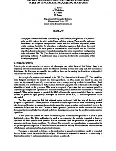
4. CASE EXAMPLE As an extensive test for the allocation and scheduling models a case example was derived, analysed, allocated (using simulated annealing) and then implemented on a DIA system. An eight node configuration was used. The topology of this configuration is shown in Figure 1; the lines in this figure represent dual port memory links between nodes. The two lines extending to the right are links to other processors. These enable the code to be down-loaded and are used as sources of sporadic events when the system is running. Each of the eight nodes receives a regular clock interrupt (into the KEC chip not the processor) from a single source. This removes clock drift but is not a fundamental feature of the DIA architecture; larger configurations may use different techniques. Nothing in the analysis presented in this paper assumes a single source of clock information. Each process’s computation time is obtained by analysis of the assembler produced for each process. Standard techniques are used9, 8, 13. Basic blocks are analysed to obtain their execution times — these are then combined using annotations such as maximum number of iterations for repeated blocks. In the prototype implementation a processor with a prefetch buffer was used. By exploiting knowledge about when preemptions can, and cannot, occur it is possible to produce a model4 that is
less pessimistic than one that ignores the benefit of the prefetch. Timings indicate that overestimation can be reduced from over 20% to under 2%.
6
4
2
0
7
5
3
1
Figure 1: An 8 node DIA System On this 8 node platform a process set consisting of 10 transactions and 42 application processes was mapped. The transactions were chosen so that routing using copy processes would be necessary. A number of processes have restrictions placed on their location. Figure 2 shows the precedence relationships between the processes. Each process is represented by a circle with its unique number contained within its circle. A "Z" on the line between two processes implies that the completion of the process on the left will trigger the release of the process on the right. This communication is called a signal. The other form of communication is called a pool and is a fully asynchronous interaction. All the initial processes in a transaction, except process 26, which is sporadic, are cyclic. The first processes in a transaction are input processes and are generally constrained to a subset of the even numbered processors. The final process in a transaction is an output process and is generally restricted to a subset of the odd numbered processors. An initial allocation of processes to processors had 15 routing agents (AGTs). This allocation was infeasible because process 49, an AGT, could not be guaranteed within its period. Simulated annealing was undertaken with 70 percent of moves being priority moves and both executive and application processes being scheduled using a unique priority algorithm. The weights for the energy function were 10 for each excess byte of private memory, 50 for each byte of excess shared memory, 2500 per excess pool/signal, 2 for the square of the number of application processes and 5000 for each process that has no deadline. A limit of 1000 attempts per temperature was imposed and the random number seed used was 32455. Figure 2 shows (above the circle) the allocation indicated after an annealing run of 186801 moves. The figures in brackets indicate the processor that each process was initially allocated to in move 1. It should be noted that where possible the tool has placed processes in a transaction close to each other. The final solution required two agent processes, 42 and 43. The tool also produces the response times which each transaction can guarantee to complete within. Each processor has a priority ordered set of processes on it and the total amount of private memory used per processor is produced. Similarly, each link has the amount of shared memory utilised produced. Three links are not used in the final configuration. Altogether, there are 44 application processes 4 clock servers and 24 servers in the final solution. A server process is needed when an application process on one processor triggers the release of a process on a connected processor. No more than 7 application processes are on any one processor.
0(2) 0
0(5)
3(3)
1
2
3(1) 3
cyclic 3 (3) 39
2(4) 4
3(2)
5(4)
5(5)
36
37
38
2(0)
2(6)
2(6)
5
6
7
2
4(4)
5(5)
42
11
12
1(5) 8
cyclic 0(0) 9
0(4) 10
cyclic 4(2)
6(4)
13
14
6(4) 15
7(0) 16
7(3)
5(5)
17
18
5
3(3)
43
40
4(2)
7(7)
34
35
cyclic 5(5) 19 4(0)
5(5)
20
21
cyclic 6(7)
6(6) 22
6(3)
7(7)
23
24
25
0(0)
2(2)
4(4)
6(6)
26
27
cyclic
28
29
0(0) 41
sporadic 1(1) 30
1(2) 31
2(5)
4(2)
32
33
cyclic Figure 2: Final Allocation
5. CONCLUSION In this paper general analysis has been presented that enables statically allocated hard real-time distributed systems to be assessed. The analysis is general purpose but has been used in this paper to consider point-to-point architectures where the issue of routing must be addressed (although the problems of scheduling a shared communication media can be ignored). Precedence related processes form transactions that have end-to-end timing requirements (deadlines). Transactions are either asynchronous or loosely synchronous. The allocation procedure having assigned each process to a node, and priorities to each process, uses the scheduling equations to first calculate local response times and then transaction response times. These response times are then compared with the deadline requirements to see if the allocation is feasible. Better allocations are then
searched for. The scheduling equations are based on estimating the maximum interference (and blocking) each process can experience from higher (lower) priority processes on the same node. The equations are more general than estimations based on processor utilisation. The DIA platform is used as an example of a point-to-point architecture. It has a number of features that aid implementation and analysis of real-time applications. Nodes are linked via dual port memories that allow concurrent reading and writing of data. In addition a kernel support chip undertakes all dispatching actions and thus allows the host processor to suffer little interference from system overheads. Although allocation of transactions to nodes can be done "by hand", with the scheduling equations being used to check a proposed mapping, the use of simulated annealing has proved to be profitable for automating the allocation activity. Current work is addressing the improvement of these techniques and to compare them with other approaches such as the use of genetic algorithms and stochastic evolution. References
1.
E. Aarts and J. Korst, Simulated Annealing and Boltzmann Machines, 1989.
2.
N.C. Audsley, A. Burns, M.F. Richardson and A.J. Wellings, ‘‘Hard Real-Time Scheduling: The Deadline Monotonic Approach’’, Proceedings 8th IEEE Workshop on Real-Time Operating Systems and Software, Atlanta, USA (15-17 May 1991).
3.
Burns, A, ‘‘Scheduling Hard Real-Time Systems: A Review’’, Software Engineering Journal 6(3), pp. 116-28 (May 1991).
4.
A. Burns, M. Nicholson and N. Zhang, ‘‘Worst Case Execution Time Estimation For Two-stage Pipelined Processors at Assembler Level’’, SPIRITS Deliverable Work Package T2A/3 (Dec 1991).
5.
S. Kirkpatrick, C. D. Gelatt and M. P. Vecchi, ‘‘Optimization By Simulated Annealing’’, Science 220, pp. 671-680 (1983).
6.
A. Konagaya, ‘‘New Topics in Genetic Algorithm Research’’, New Generation Computing 10(4), pp. 423-427 (1992).
7.
M.Joseph and P. Pandya, ‘‘Finding Response Times in a Real-Time System’’, BCS Computer Journal, pp. 390-395 (Vol. 29, No 5, Oct 86).
8.
C. Y. Park and A. C. Shaw, ‘‘Experiments with a Program Timing Tool Based on Source-Level Timing Schema’’, Proceedings Real-Time Systems Symposium , pp. 72-81, IEEE computer society press (December 5-7 1990).
9.
P. Puschner and C. H. Koza, ‘‘Calculating the Maximum Execution Time of Real-Time Programs’’, The Journal of Real-Time Systems, pp. 159-176 (1989).
10.
Y.G. Saab and V.B. Rao, ‘‘Combinatorial Optimisation by Stochastic Evolution’’, IEEE Transactions on Computer Aided Design 10(4), pp. 525-535 (1991).
11.
H. Simpson, ‘‘A Data Interaction Architecture (DIA) for Real-Time Embedded Multi Processor Systems’’, Computing Techniques in Guided Flight RAe Conference, Stevenage (19 April 1990).
12.
H. R. Simpson, ‘‘Four-slot Fully Asynchronous Communication Mechanism’’, IEE Proceedings on Computers and Digital Techniques 137, pp. 17-30 (January 1990).
13.
A. D. Stoyenko, C. Hamacher and R. C. Holt, ‘‘Analyzing Hard-Real-Time Programs for Guaranteed Schedulability’’, IEEE Transactions on Software Engineering 17 (8), pp. 737-749 (Aug. 1991).
14.
K.W. Tindell, A. Burns and A.J. Wellings, ‘‘Allocating Real-Time Tasks: An NP-Hard Problem Made
Easy’’, Real Time Systems Journal 4, pp. 145-165 (1992).