and synchronization of large multimedia data objects (MDOs). (such as, audio ..... These m sites are connected by a communication network. A communication ...
Allocating Data Objects to Multiple Sites for Fast Browsing of Hypermedia Documents Siu-Kai So, Ishfaq Ahmad, and Kamalakar Karlapalem Department of Computer Science The Hong Kong University of Science and Technology, Hong Kong Email:{kai, iahmad, kamal}@cs.ust.hk
Abstract Many world wide web applications require access, transfer, and synchronization of large multimedia data objects (MDOs) (such as, audio, video, and images) across the communication network. The transfer of large MDOs across the network contributes to the response time observed by the end users. As the end users expect strict adherence to response time constraints, the problem of allocating these MDOs so as to minimize response time becomes very challenging. The problem becomes more complex in the context of hypermedia documents (web pages), wherein these MDOs need to be synchronized during presentation to the end users. Since the basic problem of data allocation in distributed database systems is NP-complete, a need exists to pursue and evaluate solutions based on heuristics for generating near-optimal MDO allocations. In this paper, we i) conceptualize this problem by using a navigational model to represent hypermedia documents and their access behavior from end users, ii) formulate the problem by developing a base case cost model for response time, iii) design two algorithms to find near-optimal solutions for allocating MDOs of the hypermedia documents while adhering to the synchronization requirements, and iv) evaluate the trade-off between time complexity to get the solution and quality of solution by comparing the algorithms solution with exhaustive solution over a set of experiments.
1 Introduction Many world wide web applications require access, transfer and synchronization of multimedia data objects (MDOs) (such as audio, video, and images) [1], [4]. Moreover, the quality of services provided in presenting these MDOs to end-users has become an issue of paramount importance. End users have started expecting strict adherence to synchronization and response time constraints. Any application or system which cannot respond quickly and in timely manner in presenting MDOs to end users is at a clear disadvantage. In order to manage and present large number of hypermedia documents (web pages) and their MDOs, distributed hypermedia database systems have been proposed [16]. In fact, a set of web servers can be treated as a distributed hypermedia database system (DHDS). As the hypermedia documents may not be located at the end users sites, they need to be transferred across the communication network incurring delay (increasing response time) in presenting the MDOs of the hypermedia documents. Therefore, the allocation of the hypermedia documents and their MDOs govern the response time for the end-users. Moreover, as the MDOs in a hypermedia document need to be synchronized, the allocation should also adhere to these synchronization constraints. The main problem with existing models for synchronization requirements (such as, HyTime [5], [9], OCPN [8], AOCPN [10],
TPN [11] and XOCPN [15]; see [14] for a survey of OCPN and its variants) is that they do not provide any information about the expected number of times each state (representing MDO or hypermedia document) is needed in a unit time interval. Without this information, the total response time in the DHDS cannot be estimated. In this paper, we design and evaluate data allocation algorithms so as to optimize the response time for a set of endusers while adhering to the synchronization requirements of the MDOs presentation in DHDSs. In Section 2, we propose a graph notion to represent navigation in the hypermedia systems and we introduce OCPN modeling specification after that. In Section 3 we develop a cost model for the data allocation problem in DHDSs. In Section 4 we describe the proposed algorithms based on Hill-Climbing and probabilistic neighborhood search approaches. In Section 5, we include the experimental results, and Section 6 concludes the paper.
2 Modeling Hypermedia Documents 2.1 Navigation Model for Hypermedia Documents A hypermedia system is a directed graph DG(H,E) where H = {D1, D2, ..., Dn} is the set of vertices, each Dp representing a hypermedia document, and each directed edge from Dp to Dp’ is a link denoting access of document Dp’ from document Dp. Therefore, a user can start browsing the documents from (say) document Dp and then proceed to access document Dp’ , and so on. We have a label attached to each directed edge from Dp to Dp’ giving the probability of end users accessing document Dp’ from document Dp. These probabilities are generated by gathering statistics (about document access, and browsing through logs of users browsing activity) about end-user behavior over a period of time. Further, since a user may end browsing after accessing any hypermedia document, the probabilities of out-going edges from a vertex do not add up to 1.0, and the difference is the probability of ending the browsing at document Dp, and is shown by an edge connecting to the ground (see Figure 1). An n × n matrix navigation_prob is used to capture this information. Example 1: Suppose we have four hypermedia documents D1 - D4, Figure 1 shows the navigation model and the corresponding navigation_prob matrix. D1 D2 D3 D4 D1 0.1 D1 0 0.2 0.7 0 0.7 0.2 0.5 D2 0 0 0.6 0.3 0.1 D4 D3 0 0 0 0 0.3 0.4 0.1 D 0.5 0 0.4 0 1 D 4 D 2
0.6
3
Figure 1: Probability model of navigational links between hypermedia documents.
From the above navigational model, we can calculate the probabilities of accessing a hypermedia document Dp’ from
document Dp. This is done by considering all possible paths to Dp’ from document Dp and calculating the probability of accessing Dp’ from document Dp for each path, and taking the maximum of all these probabilities. Note that we assume each document access and browsing from one document to another to be independent events. Therefore, for a path with x edges from document Dp to document Dp’, the probability of this path is the product of x probabilities for the edges. Since there can be potentially infinitely long paths, we limit the length of the path by limiting the value of the cumulative probability given by the path to be less than a parameter value (bpl). Let R be the n x n matrix, with each element rjj’ giving the cumulative long run probability of accessing document Dp’ from document Dp. Example 1 (Cont.): From the navigation model, we can construct a tree for each document representing the possible navigation path for each session starting from that document. These are given in Figure 2. We set the bpl value to be 0.01. Notice that we do not need to further expand a node if the document represented by that node is the same as that of the root. (This happens in the first tree in Figure 2). Therefore, if we start navigating the hypermedia system from document D1, we have probability 0.2 that we browse document D2. For document D3, we have probability 0.7 if we follow the right path from D1, but probability 0.2 × 0.6 = 0.12 if we follow the path D 1 → D 2 → D 3 . In this case, we use the greater probability to represent the long run probability of browsing D3 from D1 as 0.7. Similarly other cumulative probability values are calculated. Therefore, the matrix R is D1 D2 D1 D2 D3 D4
1 0.15 0 0.5
D1
D2 0.7
0.2
D2 0.6
D3 0.3
0.5
D1
D3
D2
0.7 0.6 1 0.4
0.06 0.3 0 1 . D4 0.5
0.7
D3
0.2
0.7
D2
D3 D3
0.4
D1 0.4
D1 0.2
D4
D3
0.5 0.4
D3
D4
D3
OCPN1:
0.6
D3
D3 0.3
D4
Figure 2: Navigation path starting from each hypermedia document (bpl is set as 0.01).
2.2 Modeling Synchronization Constraints on MDOs We use the Object Composition Petri Nets (OCPNs) [8] for modeling the synchronization constraints among the MDOs in a hypermedia document. Petri nets are composed by Places (representing MDOs) and Transitions. We can transverse a Transition (called as firing) if all Places pointing to this Transition have a token and are in an unlocked state. When the Transition fires, the Places that the Transition is pointing to will become active (a token is added to these Places) and locked. Places will become unlocked when their durations have expired. All OCPN models can be mapped to a corresponding HyTime model [2]. In Figure 3, the following synchronization constraint is represented in OCPN1: MDO B has to be shown at the start of browsing the hypermedia document, and after 40 units of time
(40,15,2280)
E d1
OCPN2:
(0,30,2280)
A (0,55,1220)
A d2
(0,30,2870)
C
B OCPN3:
OCPN4:
d3
C
B
(0,80,1220)
B
(0,40,2870) (40,30,1220)
d4
(0,80,2870)
C Figure 3: The OCPN specification of each hypermedia document; the tuple is [start time, duration, media size in kilobytes].
3 Cost Model of Data Allocation Scheme Table 1 lists a number of notations used throughout this paper. Table 1: Symbols and their meanings. Symbol Meaning Si
The ith site
Dj
The jth hypermedia document
Ok
The kth MDO
m
The number of sites in the network
n
The number of hypermedia documents in the database system
k P p
0.3
0.6
D4
D3
0.2 1 0 0.1
MDO A must be shown in sync with it. The OCPN specifications of hypermedia documents D1 to D4 are shown in Figure 3.
The number of MDOs in the database system i
The user navigation pattern matrix of site i
i jj′
The probability of using document j′ as initial document if the initial documnet is j in the previous navigation session at site i
B
The navigation initial document frequencies matrix
b ij C c ii′
The frequency of using the jth document as initial point at the ith site
A a ij
The access frequencies matrix
l li
The allocation limit vector of the sites
R
The hypermedia document dependency matrix
r jj′
The transmission speed matrix of the network The transmission speed from site i to site i′ The access frequency of document j from site i The allocation limit of site i The probability of retrieving document j′ if browsing initial document is j
OCPN j
The OCPN specification of document j
U u jk
The use matrix
dur jk
The presentation duration of MDO k in document j
start jk
The presentation starting time of MDO k in document j
size k
The size of the kth MDO
bpl et j
The browsing probability limit.
D d ij
The delay matrix
t
The total delay
The boolean value of whether document j uses MDO k
The expected number of times document j will be retrieved The delay of presentation starting time of document j at site i
3.1 Overview In order to reduce response time for the end-users browsing activities, we need to develop a cost model for calculating the total response time observed. This response time depends on the location of the MDOs and the location of the end-user. Further, it depends on the synchronization constraints among the MDOs of the hypermedia document browsed. The hypermedia document
navigational model presented in Section 2.1 is used to estimate the number of accesses (times browsed) to each MDO from each site. This gives us information regarding affinity between the MDOs and the sites of the distributed environment. Typically, one would assign a MDO to a site which accesses it most. But this may incur large delay for other sites which need to access this MDO. Further, synchronization constraints may impose additional delays in transferring the MDO to the end-user site. This is done when two streams of MDOs need to simultaneously finish their presentation, and one of them is for shorter duration than the other. Since we are buffering the MDOs at the user sites before the start of the presentation, the MDO allocation problem needs to minimize this additional delay that is incurred because of the synchronization constraints. We also take into consideration limited buffer space constraint at end-users site and user interaction during MDO presentation.
3.2 Total Response Time Cost Function Suppose there are m sites in the distributed hypermedia database system. Let S i be the name of site i where 1 ≤ i ≤ m . These m sites are connected by a communication network. A communication link between two sites S i and S i′ will have a positive integer c ii′ associated with it giving the transmission speed from site i to site i′ . Notice that these values depend on the routing scheme of the network. If fixed routing is used, we can have the exact values. However, if dynamic routing is in used, we can only obtain the expected values. Let there be n hypermedia documents, called { D 1, D 2, …, D n } accessing k MDOs, named { O 1, O 2, …, O k } . From the navigation model, we can construct n trees representing the navigation path of the session starting from each document. As in Section 2.1, we must limit the level we will use for our cost model by a threshold value bpl, say 0.001. These trees will give us some information about the probability r jj′ of retrieving document D j′ if we start navigating from D j . For each site, we use an irreducible continuous-timed Markov process [13] to model the user behavior in initial browsing document (i.e., the document first browsed) as a i stationary regular transition probability matrix, P ,1 ≤ i < m . These processes will converge in the long run and from these long run behaviors, we can estimate the probability of browsing each document from each site as the initial browsing document. These Markov chains will have n + 1 states representing the probabilities of using each of the documents as the initial browsing document (n states), and probability of not browsing any of the documents ( (n+1)th state). Normalize the probabilities derived from long run behavior Markov chain at each site and multiply them by a constant S, we have the expected frequencies of initial document out of S browsing sessions. The resultant information is represented by an m × n matrix B. We multiply this matrix to the n × n matrix R obtained from the hypermedia document trees to generate an m × n matrix A with entries a ij giving the expected number of times S i needs to retrieve the MDOs in D j . Further, we need the starting time, duration, size, and presentation rate of each MDO in each hypermedia document. This information can be obtained from the OCPN specification of MDOs in a hypermedia document.
A box will be added at the beginning of each OCPN which represents the delay in starting the presentation of the hypermedia document so as to adhere to the synchronization requirements. The duration of this delay box is related to the browsing site and the sites where the MDOs in the document are allocated. Thus, we use d ij to represent the duration of the delay box when site S i accesses document D j . From the OCPN representations, we have the starting time start jk and duration dur jk of each MDO O k in each document D j . In addition, the n × l usage matrix U is generated from the OCPN specifications. If document D j uses MDO O k , then set u jk to 1, otherwise, set u jk to 0. Then, by multiplying A by U, we can estimate the access frequencies of each MDO from each site. Let size k be the size of MDO O k . With this information, we can calculate d ij by, size d ij = max ∀k, u jk = 1(--------------k- – dur jk – start jk) EQ 3.1 c site(k) ⋅ i where site(k) represents the site where O k is allocated. We can calculate the values of all d ij, 1 ≤ i ≤ m, 1 ≤ j ≤ n , by using the above formula. This formula means that the delay is equal to the maximum value of (transmission duration presentation duration - presentation starting time) for each MDO in the document. A negative value implies that the transmission time is shorter than the presentation time, we can start presenting the MDOs in the hypermedia document as soon as the MDOs arrive at the end-user site. A positive value implies that we must delay the presentation, otherwise the MDOs presentation will end after the synchronization time, and hence will not adhere to the synchronization constraints. Therefore, we have the cost function, EQ 3.2 t = ∑ ∑ d ij ⋅ a ij i∈Sj∈D
By minimizing this value through the change of the function site(k) , we obtain the data allocation scheme that is optimal (the (delay incurred) response time is minimal), while adhering to the synchronization constraints.
3.3 User Interactions and Buffer Space Constraints The model presented above does not consider user interactions and buffer space constraints. It assumes that the user does not interrupt the presentation and the size of the local storage facility is large enough for storing any one of the hypermedia documents in the hypermedia database system. By including user interactions and buffer space constraints, there can be four different cases for hypermedia document allocation problem given below.
No user interaction and unlimited buffer space: This is essentially the best scenario, because we can retrieve all MDOs in a hypermedia document at the beginning since there is no storage limitation. As there is no user interaction, the data can be discarded immediately after use. The cost function for the response time for each hypermedia document, as presented in Section 3.2, is the maximum of the delays of the embedded MDOs for satisfying the synchronization requirements. User interaction and unlimited buffer space: By including user interactions, some of the MDOs in a hypermedia document may need to be presented multiple times (e.g. play in
reverse or stop and resume later). However, as there is unlimited buffer space, the system can store all MDOs of a hypermedia document once they are retrieved. Therefore, the delay for handling the user interactions is some local processing time that is irrelevant to the data allocation of the MDOs. The cost function is thus same as that in the Section 3.2.
No user interaction and limited buffer space: In this scenario, the system can not use the retrieving all the MDOs in advance strategy. Instead, the system must retrieve the MDOs only when it needs to present these MDOs. Therefore, every synchronization point in the hypermedia document may cause some delay and the cost function in such situation is the summation of these delays. Indeed, the model presented in Section 3.2 can be generalized to deal with this scenario. First, we need to decompose each document into component sub-documents. From the OCPN specifications, we have the states representing the MDOs in each document. Denote this set of states as S and for ∀s, s ∈ S , we can get the starting time and ending time of the state (i.e., presentation of the corresponding MDO) from the OCPN specifications. Then, we can decompose the document by composing all MDOs starting at the same time into a sub-document (so if there are h MDOs, there will be h subdocuments in maximum).
User interaction and limited buffer space: If we know the expected number of times each sub-document will be presented in each hypermedia document, we can calculate the expected response time of each document in each site. It is just the weighted sum of the delays of the sub-documents in the document. To calculate the expected number of times each document is needed, we must know the probabilities of relevant user interactions (such as reverse playing, and fast forward). Once we have these probabilities, we can calculate the expected number of time each document is presented by employing the first step analysis method [13]. Note that these probabilities can be generated by observing user interaction over a period of time. For example, suppose the relevant probability of an MDO k in a document j is ip jk . Assume that the expected number of time this MDO is needed is mdo_et jk . Then, we have†, mdo_et jk = 1 + ip jk × mdo_et jk, mdo_et jk = ( 1 – ip jk )
–1
EQ 3.3
Similarly, we can estimate the expected number of times other MDOs composing this document are needed. Then, the expected number of times this document is needed is just the maximum of these values. Denote this value as et j for document D j , we have, et j = max(mdo_et jk), for ∀k, u jk = 1 EQ 3.4 And the delays d ij will become, size d ij = max(--------------k- – dur jk – start jk) ⋅ et j, for ∀k, u jk = 1. c site(k) ⋅ i Example 1 (Cont.): Assume that the hypermedia database system is distributed in a network with 3 sites. In Figure 4, the transmission speed between the 3 sites are given. These values can be represented as an m × m matrix C, with entry c ii′ representing the transmission speed from S i to S i′ . †. or mdo_etjk = 1 + ipjk + ipjk2 + ... = (1 - ipjk)-1.
S1 41
38 35
S2 S3 Figure 4: The transmission speed between the sites in Kilobytes per second. S1 S2 S3 S1 0 38 41 S2 38 0 35 S3 41 35 0 . Suppose after the analyses of the long run behavior of the Markov chain in each site, the expected starting document frequencies out of S = 900 browsing sessions, matrix B is, D1 D2 D3 D4 S1 100 200 300 200 S2 225 450 225 0 S3 300 100 100 400 . Then the matrix A ( B × R ) is, D1 D2 S1 S2 S3
245 292.5 515
340 495 200
D3
D4
630 652.5 530
296 148.5 448 . In this example, there are 3 MDOs, namely A, B and C (E is a delay state, so there is no associative actual MDO). If we allocate A at Site 2, B at Site 3 and C at site 1, then d 11 is equal to, 1220 2280 d 11 = max ------------ – 15 – 40 , ------------ – 55 – 0 = 5. 38 41 Similarly, we can calculate the values of all d ij, 1 ≤ i ≤ 3, 1 ≤ j ≤ 3 when we have the MDO allocation scheme. And the total response time delay will be, t = 11430 + 4573.25 + 29130 = 86291.25. Suppose we add user interactions and worst case buffer space constraints to this hypermedia database system. After adding the probability of relevant user interruption to the MDO, the augmented OCPN of D1 is shown in Figure 5. OCPN1 : d1
(40,15,2280)
E
A 0.4
0.5
B (0,55,1220) Figure 5: The augmented OCPN by including user-interaction. Thus, the expected number of times MDO A is needed when document D1 is retrieved is, mdo_et 1 A = 1 + 0.4 × mdo_et 1 A, –1 mdo_et 1 A = ( 1 – 0.4 ) = 1.667. Similarly, the expected number of times MDO B is needed is, mdo_et 1B = 1 + 0.5 × mdo_et 1B, –1 mdo_et 1B = ( 1 – 0.5 ) = 2. Notice that when we need B again, A is also needed. Thus, et 1 = max(1.667, 2) = 2 . Since we have worst case buffer space constraints, so the delay d 11 will become 1220 2280 d 11 = max ------------ – 15 – 40, ------------ – 55 – 0 × 2 = 10. 38 41
4 Proposed Data Allocation Algorithms The data allocation problem in its simple form has been shown to be NP-complete [3] and the problem discussed here is m more complex than the simple case; there are k different allocation schemes for a system with m sites and k MDOs, implying that an exhaustive search would require O ( k m ) in the worst case to find the optimal solution. Therefore, we must use heuristic algorithms to solve the problem.
4.1 The Hill-Climbing Approach We have developed an algorithm based on the Hill-Climbing technique to find a near optimal solution. The data allocation problem solution consists of the following two steps: 1) Find an initial solution. 2) Iteratively improve the initial data allocation by using the hill climbing heuristic until no further reduction in total response time can be achieved. This is done by applying some operations on the initial allocation scheme. Since there are finite number of allocation schemes, the heuristic algorithm will complete its execution. For step one, one possibility is to obtain the initial solution by allocating the MDOs to the sites randomly. However, a better initial solution can be generated by allocating an MDO to the site which retrieves it most frequently (this information can be obtained from the matrix A × U ). If that site is already saturated, we allocate the MDO to the next site that needs it the most. We call this method the MDO site affinity algorithm. In the second step, we apply some operations on the initial solution to reduce the total response time. Two types of operations are defined, namely migrate and swap (see below). These operations are iteratively applied until no more reduction is observed in the total response time. migrate ( O j, S i ) : move MDO O j to S i . This operation can be applied to each MDO, and an MDO can be moved to any one of the m – 1 sites at which it is not located. Therefore, there can be a maximum of k ( m – 1 ) migrate operations that can be applied during each iteration. swap ( O x, O x′ ) : swap the location of MDO O x with the location of MDO O x′ . This operation can be applied to each distinct pair of MDOs. Therefore, there can be a maximum of k ( k – 1 ) ⁄ 2 swap operations that can be applied during each iteration.
4.2 The Random Search Approach One drawback of the Hill-Climbing approach is its high complexity. Another problem is that the algorithm can be trapped in some local minimum. This is because the exchange or migration of MDO is done only if the movement will give a better solution. To increase the chance of finding the global optimal solution, we must introduce some probabilistic jumps [6], [7]. The probabilistic jumps must be large enough by involving MDOs that can have a great effect on the solution quality. Otherwise, if the jump is small, the algorithm may be remain trapped in the same local minimum. Thus, before the execution of the algorithm, we must determine which subset of the MDO set is important. One possible set of important MDOs is the MDOs which are presented at the beginning of some hypermedia document. The reason being that when we browse a hypermedia
document, we must retrieve and use the starting MDO immediately, so their transmission delay will have a great effect on the overall document presentation delay. Thus, we have two sets of MDOs: critical MDOs (CMDOs) and non-critical MDOs (OMDOs). The random algorithm starts with an initial solution using the site affinity algorithm and then constructs the two MDO sets. It then tries to merge OMDOs to some random sites by using either the migrate operation or the swap operation whichever gives more improvement in the solution quality. It continues to do so for MAXSTEP times but will stop if there is no improvement in MARGIN number of trials. It then chooses one of the CMDOs and migrate it to a random site or swap it with another randomly selected CMDO. This is repeated for MAXCOUNT times. The algorithm preserves the best solution found so far and then does a neighborhood search on CMDOs again to see if there is further improvement. The worst-case running time of the algorithm is O(MAXSTEP × MAXCOUNT ) . It is reasonable to set MAXSTEP as a multiple of the number of OMDOs and the number of sites. Similarly, MAXCOUNT is set to be a multiple of the number of CMDOs and the number of sites. MAXSTEP = a ⋅ 〈 m ⋅ OMDOs 〉 MAXCOUNT = b ⋅ 〈 m ⋅ CMDOs 〉 2
2
With these assumptions, we will have an O(m k ) algorithm.
5 Results In this section, we present the experimental results for the data allocation algorithms described in Section 4. Comparisons among these algorithms will be made by considering the quality of solutions and the algorithm running time. Since for k MDOs and m sites there are k m allocation schemes for exhaustive search algorithm, the problem sizes of the experiments we conducted were limited. We conducted 10 experiments with number of MDOs ranging from 4 to 8, and number of sites ranging from 4 to 8. Each experiment consisted of 100 allocation problems with the number of sites and the number of MDOs fixed. Each allocation problem had between 4 and 16 documents, and each document used a subset of the MDOs with its own temporal constraints on them. The communication network, the MDO sizes, the link costs, and the temporal constraints between MDOs in each document were randomly generated from a uniform distribution. The two data allocation algorithms described above were tested for every case and statistics was collected. In Table 2, for each of the experiments conducted in a column-wise fashion, we list the following: i) the number of sites, ii) the number of MDOs, iii) the number of problems for which optimal solutions are generated by hill-climbing, iv) the average deviation in percentage of near optimal solutions from optimal solution when optimal solution was not reach, v) and vi) provide similar results for random search algorithm. The number of optimal solutions can reflect how good the algorithm is; whereas the average deviation shows how bad the algorithm performs when it cannot generate optimal solution.
Table 2: Experimental results of the two algorithms. No. of No. of No. of Opt. Aver. % No. of Opt. Sites MDOs Sol. (H) Deviat. (H) Sol.(R)
6 Conclusions Aver. % Deviat. (R)
4
4
93
15.4163
98
11.0071
4
8
81
5.3714
70
5.0961
5
4
92
19.3567
97
1.1011
5
8
83
11.5364
62
5.6252
6
4
97
5.2258
92
4.8935
6
8
82
11.6584
56
2.8690
7
4
88
3.0582
86
1.8645
7
8
77
3.9969
62
4.4913
8
4
88
3.8620
90
1.5051
8
8
72
9.7750
50
3.6533
From Table 2, we note that the Hill-Climbing algorithm generated optimal solutions for a large number of problems — 853 cases out of a total of 1000 cases, corresponding to about 85% of the test cases. Most of the non-optimal solutions are in the range of 0-5% deviation from the optimal solution while a few solutions are in the range of equal to or more than 20%. The average percentage (only for non-optimal cases) is about 7.9384 across all cases. These results indicate that the Hill-Climbing algorithm is able to generate high quality solutions in comparison to random search algorithm. It seems that the algorithms cannot handle case with large problem space such as thousands MDOs (running time is too long). In such case, we can group MDOs into clusters and use the algorithms to allocate the clusters instead of individual MDOs.
5.1 Comparison of Running Times Table 3 contains the average running times of both algorithms for each experiment. For comparison, the time taken to generate the optimal solutions by using exhaustive search are also listed. All the algorithms were implemented on a SPARC IPX workstation and the time data was measured in milliseconds. As can be seen from the table, although the Random Search algorithm took much short time compared with exhaustive search and about 1 order of magnitude less time than the Hill-Climbing Approach. Such margins become highly significant when the problem size is large. Therefore, while the Hill-Climbing algorithm may be preferred for small problem sizes, the Random algorithm would be a better choice for large problem sizes. From the experiment results presented in the previous section, we observe that there is a trade-off between execution time and solution quality. The random search algorithm is very cost-effective if fast execution is desired. If the solution quality is the more prominent factor, the Hill-Climbing approach is a viable choice for an off-line allocation. Table 3: Average running times (msecs) of all algorithms. No. of No. of Exhaustive Hill Random Sites MDOs Search Climbing Search 4
4
7.63
38.95
27.44
4
8
6457.69
1014.08
183.12
5
4
18.34
68.36
45.57
5
8
50224.66
2011.78
314.17
6
4
51.88
85.14
67.28
6
8
273494.96
2885.52
446.66
7
4
176.10
166.09
97.67
7
8
1587830.28
4721.17
620.85
8
4
333.23
169.28
134.06
8
8
5755754.63
12053.53
875.84
A probabilistic navigational model for modeling the user behavior while browsing hypermedia documents is developed. This model is used to calculate the expected number of accesses to each hypermedia document from each site. Synchronization constraints for presenting the MDOs of hypermedia documents are modeled by using the OCPN specification. A cost model is developed to calculate the average response time observed by the end-users while browsing a set of hypermedia documents for a given allocation of MDOs. This cost model is generalized to take into consider end-user interaction while accessing MDOs, and limited buffer space constraints at the end-user site. After that, two MDO data allocation algorithms, one based on Hill-climbing heuristic, and other based on Probabilistic Random search are proposed. The two algorithms use extreme approaches: a high complexity extensive incremental strategy and a fast random search. Results indicate that there is a trade-off between execution time and solution quality. The random search algorithm is cost-effective if fast execution is desired. If the solution quality is the more prominent factor, the Hill-Climbing approach is a viable choice for small problem sizes.
References [1] P. B. Berra, C. Y. R. Chen, A. Ghafoor, C.C. Lin, T. D. C. Little, and D. Shin, “Architecture for Distributed Multimedia Systems”, Computer Communications vol.13, no.4 (May 1990) p217-31. [2] R. Erfle, “HyTime as the multimedia document model of choice,” Proc. of the Int. Conf. on Multimedia Computing and Systems, Cat. No. 94TH0631-2, 1994, pp.445-454. [3] K. P. Eswaran, “Placement of Records in a File and File Allocation in a Computer Network,” Information Processing, 1974, pp.304-307. [4] A. Ghafoor, “Multimedia database management systems,” ACM Computing Surveys, 27(4) Dec. 1995, pp.593-598. [5] C.F. Goldfarb, “Standards-HyTime: a standard for structured hypermedia interchange,” IEEE Computer, 24(8), 1991, 81-84. [6] D.S. Johnson, C.H. Papadimitriou and M. Yannakakis, “How Easy Is Local Search,” Journal of Computer and System Sciences, vol. 37, no. 1, Aug. 1988, pp. 79-100. [7] Y.-K. Kwok, I. Ahmad, and J. Gu, “FAST: A Low-Complexity Algorithm for Efficient Scheduling of DAGs on Parallel Processors,” Proc. of ICCP, Aug. 1996, vol. II, pp. 150-157. [8] T. D. C. Little, “Synchronization and storage models for multimedia objects,” IEEE JSAC, 8(3) April 1990, pp.413-427. [9] S. R. Newcomb, “Multimedia interchange using SGML/ HyTime,” IEEE Multimedia, 2(2) 1995, pp. 86-89. [10] B. Prabhakaran and S. V. Raghavan, “Synchronization models for multimedia presentation with user participation,” Multimedia Systems, 1994, vol. 2, pp.53-62. [11] J. Song, Y. N. Doganata, M. Y. Kim and A. N. Tantawi, “Modeling Timed User-Interactions in Multimedia Documents,” Proc. Int. Conf. on Multimedia Computing and Systems, 1996, pp.407-416. [12] P. D. Stotts and R. Furuta, “Petri-net-based hypertext: document structure with browsing semantics,” ACM TOIS, 7(1) 1989, pp.3-29. [13] H. M. Taylor and S. Karlin, An Introduction to stochastic modeling, Academic Press, 1994. [14] S. Vuong, K. Cooper and M. Ito, “Specification of Synchronization Requirements for Distributed Multimedia Systems,” Proc. Int.l Workshop on Multimedia Software Development, 1996, pp.110-119. [15] M. Woo, N.U. Qazi, and A. Ghafoor, “A Synchronization Framework for Communication of Pre-orchestrated Multimedia Information,” IEEE Network, pp. 52-61, January/ February 1994. [16] G. R. Rao, V. Balasubramanian and B. A. Suresh, “Integration of Hypertext and Object-Oriented Databases for Information Retrieval,” Proceedings of the 1993 IEEE Nineteenth Annual Northeast Bioengineering Conference, May 1993, pp. 201-204.