November 18, 2009
15:34
WSPC - Proceedings Trim Size: 9.75in x 6.5in
announcement
1
Almost dense orbit on energy surface Vadim Kaloshin1,2 , Ke Zhang1 and Yong Zheng1 1 Department of Mathematics University of Maryland at College Park MD, USA, 20740 2 Department of Mathematics, Penn State University, PA, USA, 16801, emails:
[email protected],
[email protected],
[email protected] We study a C r nearly integrable Hamiltonian system Hε (q, p) = 12 !p, p" + !H1 (q, p) defined on T3 × R3 . Let Σ = {(q, p) : Hε (q, p) = 12 } and µΣ1 be the restriction of Lebesgue measure on T3 × R3 to Σ. We prove there is a perturbation H1 (q, p) ∈ 3 3 C r , %H1 %C r ≤ 1 and an orbit (q(t), p(t)) S : R → T × R of the Hamiltonian equation {q˙ = ∂p Hε , p˙ = −∂q Hε } such that µΣ ( t∈R (q(t), p(t))) ≥ 21 .
1. Introduction The famous question called the ergodic hypothesis suggested that for a typical Hamiltonian on a typical energy surface all, but a set of zero measure of initial conditions, have trajectories covering densely this energy surface itself. However, KAM theory showed that for nearly integrable systems there is a set of initial conditions of positive measure of quasi periodic trajectories. This disproved the ergodic hypothesis and forced to reconsider the problem. A quasi ergodic hypothesis asks if a typical Hamiltonian on a typical energy surface has a dense orbit. A definite answer whether this statement is true or not is still far out of reach of modern dynamics. There was an attempt to prove this statement by E. Fermi,5 which failed (see6 for more detailed account). To simplify the quasi ergodic hypothesis, M. Herman7 formulated the following question: Can one find an example of a C ∞ Hamiltonian H in a C r small neighborsuch that on the unit energy surface {H−1 ( 21 )} there is a dense hood of H0 (p) = "p,p# 2 trajectory? Many people believe that such examples do exist and are C ∞ –generic (see,4 ,31 ). In this paper we make a step in the direction of answering Herman’s question. For any r we construct a Hamiltonian, which is C r close to H0 (p) = "p,p# and has 2 a trajectory dense in a set of Lebesgue measure 1/2 on the energy surface. Here is the exact statement. Let q ∈ T3 , p ∈ R3 and H0 (p) = "p,p# be the unperturbed 2 Hamiltonian, where "p, p# is the dot product in R3 . Theorem 1.1. For any r ≥ 2 there is a C r small perturbation Hε (q, p) = H0 (p) + !H1 (q, p, !) and an orbit (q(t), p(t)) : R → T3 × R3 of q˙ = ∂p Hε ,
p˙ = −∂q Hε
(1)
November 18, 2009
15:34
WSPC - Proceedings Trim Size: 9.75in x 6.5in
announcement
2
! such that µΣ ( t∈R (q(t), p(t))) ≥ 21 .a
Let Σ = {(q, p) : H" (q, p) = 21 }, we fix a subset F ⊂ Σ with µΣ (F ) ≥ 12 . It suffices to prove that for any δ > 0 there exists Tδ such that the δ neighborhood of ! t∈[0,Tδ ] (q(t), p(t)) contains F . We will construct Hε in two steps. In step one we build Hε& = H0 + εH1& so that has a variety of good local normal forms and nice invariant sets. Then Hε = Hε& +εH1&& is designed to have diffusing orbits shadowing these invariant sets. 2. Choice of F We will describe the choice of the positive measure set F , as well as an approximate path of diffusion. We begin with a informal discussion of the diffusion path and what kind of perturbation we need. Usually diffusing orbits travel along resonant segments. To be able to saturate a set of positive measure one has to be able to move along infinitely many resonant segments. If size of a perturbation is fixed, the analysis of motions near resonances of larger and larger orders in the original coordinate system becomes increasingly complicated as explained in section 4 . To be able to control dynamics along some arbitrary high order resonant we define a convenient symplectic coordinate system Φ : (θ, I) → (q, p) on a neighborhood of {)p) = 1, p1 ≥ 12 }, such that Hε& ◦ Φ(θ, I) = H0 (I) + H1 (θ, I), where )H1 (θ, I))C r gets the smaller as the order of a corresponding resonance increases. We consider the following set of Diophantine numbers: Dγ = {ω = (ω1 , ω2 , ω3 ); )ω) = 1, |k · ω| ≥ γ|ω||k|−2−τ , ∀k ∈ Z3 ; |k1 ω1 + k2 ω2 | ≥ γ δ(1+δ) |(k1 , k2 )|−1−δ , ∀(k1 , k2 ) ∈ Z2 ; |k1 ω1 + k3 ω3 | ≥ γ
δ(1+δ)
−1−δ
|(k1 , k3 )|
(2)
2
, ∀(k1 , k3 ) ∈ Z },
where δ > 0 is a small number. The set Dγ has positive measure on the surface {)ω) = 1}. Let B = {)ω) = 1; ω1 ≥ 21 } and we will choose a subset Dγ∞ ⊂ Dγ ∩ B with positive measure. The family of Diophantine number corresponds to a family of KAM tori which has measure on the energy surface {H" = 12 }. Denote it F . The construction will be done in infinitely many stages, each stage we will define a set of paths in the set B, such that if the Hamiltonian H satisfies a list of properties, there exists an orbit such that ϕ˙ shadows the chosen path. The path gets denser in each stage and in the limit ϕ˙ accumulates to a set of positive measure. For any integer vector k ∈ Z3 \ {0}, we can relate to it a resonant plane {ω ∈ R3 : k · ω = 0}. If the plane intersects B, the intersection is a curve on the unit sphere, which we will refer to as Γk . At stage 1 the construction consists of the following components: a In8
there is a construction of Hε and an orbit of Hε whose closure has maximal Hausdorff dimension
November 18, 2009
15:34
WSPC - Proceedings Trim Size: 9.75in x 6.5in
announcement
3
(1) Let γ1 = γ 4 . We will choose a discrete set DN 1 ⊂ Dγ ∩ B, and disjoint neighborhoods U(ωi ) of ωi ∈ DN 1 , such that each U(ωi ) contains a ball of radius γ1 , and is contained in a ball of radius 3γ1 , both centered at ωi . ! (2) Let Dγ1 = Dγ ∩ ωi ∈DN 1 U(ωi ), we have the sets U(ωi ) is chosen in such that a way that the measure of Dγ \ Dγ1 is small. (3) There exists a collection F1 of integer vectors, such that for any ωi ∈ DN 1 there exists some k ∈ F1 such that Γk enters γ1 /2 neighborhood of ωi . Furthermore, ! the union F 1 := k∈F1 Γk is connected. In stage 2, let γ2 = γ11+α for some α > 0. For each neighborhood U(ωi ) of stage 1, we similarly define the following:
(1) A discrete set DN 2i ⊂ Dγ1 ∩ U(ωi ), and for each ωij ∈ DN 2i , we have neighborhoods U(ωij ), whose radius is between γ2 and 3γ2 . ! (2) Di2 = Dγ1 ∩ ωij ∈DN 2 U(ωij ). The measure of Dγ1 ∩ U(ωi ) \ Di2 is small. i (3) For the neighborhood U(ωi ), there exists k & ∈ F1 , such that the resonant line Γk! enters the neighborhood. We further define a collection F2i of integer vectors, such that for any ωij ∈ DN 2i , there exists some k ∈ F2i such that Γk enters ! γ2 /2 neighborhood of ωij . Write Fi2 = k∈F1 Γk , we assume that Fi2 ∪ Γk! is i connected. Denote also Fn = ∪ni=1 F i . ! ! We do this for every neighborhood U(ωi ) and let DN 2 = DN 1i , Dγ2 = Di2 , ! ! F2 = F2i , F 2 = Fi2 . We then continue this construction inductively: for each multi-index (i1 · · · in ), assume that we have the neighborhood U(ωi1 ···in ), we can n+1 n+1 define DN n+1 i1 ···in , Di1 ···in and Fi1 ···in in a similar fashion. Union over all multi-indices of same order is denoted by DN n+1 , Dγn+1 and Fn+1 . Then Dγ∞ is the intersection of Dγn and has almost full measure in Dγ ∩ B. Finally, using ideas from,15,16 we have the following Theorem 2.1. The Hamiltonian H(θ, I) = H0 (I) + H1 (θ, I) has the following property: Consider the resonant lines F n of stage n, there exists an open cover Uj of F n , such that for each Uj , there exists a neighborhood Uj × T3 ⊃ (∂I H)−1 (Uj ), on which H is in one of the two normal forms: ˆ I) ˆ → (θ, I) (1) Single and ghostb resonances: There exist local coordinates Ψ : (θ, such that ˆ I) ˆ + R, ˆ =H ˆ 0 (I) ˆ + ak cos(πk · θ) H ◦ Ψ(θ,
n
(3)
where k ∈ F and )R) / |ak |. (2) Double resonance: H(θ, I)|Uj × T3 = H0 (I) + ak cos(πk · θ) + ak! cos(πk & · θ) + R, n
&
where k ∈ F , k is in F
n−1
n
, F or F
n+1
(4)
, )R)C 3 / max{|ak |, |ak! |}.
are certain k "" *∈ Fn−1 ∪ Fn ∪ Fn+1 such that Γk intersects Γk!! inside Uj . We call such an intersection a ghost double resonance
b there
November 18, 2009
15:34
WSPC - Proceedings Trim Size: 9.75in x 6.5in
announcement
4
3. A proof of existence of a δ−dense orbit using a variational problem with constrains In this section we reformulate a problem of existence of an orbit following a Cantor set of lines as a variational problem with constrains (following Mather). Recall that under the convenient coordinate system we have the Hamiltonian H(θ, I) = H0 (I) + H1 (θ, I). Due to the convexity with respect to I, the Hamiltonian system (1) is equivalent ˙ = l0 (θ)+L ˙ ˙ to the dynamics of the E-L equation with Lagrangian L as L(θ, θ) 1 (θ, θ), 3 ˙ which is positive definite with respect to θ for any θ ∈ T . n k k+1 n Select {ωnk }N k=1 be a set of points in F such that |ωn − ωn | is sufficiently small. Denote by Aω a special invariant set of orbits (to be defined later) with rotation vector ω. In our case velocity of these orbits will stay close to ω. Our goal is to k n construct a transition chain from these sets {Aωn }N k=1 and an orbit shadowing k these sets. Such an orbit will stay close to the union of the stable set W s (Aωn ) k and the unstable set W s (Aωn ) for all time. We find these orbits by constructing a variational problem with constrains. This construction is fairly involved and relies heavily on Mather’s ideas. We describe its construction into several steps. Let θ ∈ T3 , denote θˆ ∈ R3 a lift to R3 . Let η be a closed one form, denote ηˆ a lift of it to a periodic close one form on R3 . Fix a lift. One can proof existence of the following set of objects: collections of numbers αi , periodic functions Bi± and closed one forms ηi on the 3-torus T3 , errors (negligibly small numbers) δi , smooth manifolds Si with a boundary diffeomorphic to a 2–disk inside the 3-torus T3 such that the following variational problem with constrains has an interior solution: Given T ∗ 0 1 and T 0 N T ∗ , consider M (θ0 , . . . , θN ) =
N "
min
θi ∈Si , Ti+1 −Ti ≥T ∗ i=0 T0 =0,TN =T
where hi (θi , θi+1 , T ) = min
#
0
hi (θi , θi+1 , Ti+1 − Ti ),
(5)
T
(L − ηc )(γ(s), γ(s)) ˙ dt,
(6)
and the minimum is taken over all absolutely continuous curves γ : [0, T ] → T3 such that γ(0) = θˆi = θi (mod1), and γ(T ) = θˆi+1 = θi+1 (mod1). In addition, we need some constraints on the homology class of the minimizing orbit, which can be achieved by going to a proper covering of T3 . We clarify this later in the section. It turns out that for each i = 0, . . . , N we have |hi (θi , θi+1 , ∆Ti ) − αi (Ti+1 − Ti ) + Bi− (θi ) + Bi+ (θi+1 )| ≤ δi . Thus, to have an interior minimum it suffices to have a sufficiently deep interior minimum of Bi− (θi ) + Bi+ (θi+1 ). It also turns out that ηi and ηi+1 can be chosen so that they coincide near the disk Si+1 .
November 18, 2009
15:34
WSPC - Proceedings Trim Size: 9.75in x 6.5in
announcement
5
Having this as the motivating goal, we shall define related objects from the Mather theory(13,14 ). Here is the correspondence: Bi± (θ) are one-sided barrier functions, defined by Mather.9 These functions form a 3-parameter family, naturally parametrized by c ∈ H 1 (T3 , R). It turns out that cohomology class of the one form ηi is given by [ηi ]H 1 (T3 ,R) = ci . To determine position of Si ⊂ T3 we need to determine a location of certain invariant sets, usually called Aubry sets Aci also naturally parametrized by c. Let I = [a, b] be an interval of time and c ∈ H 1 (T3 , R) = R3 . A curve γ ∈ C 1 (I, T3 ) is called c−minimizer if # b # b Ac (γ) := (L − ηc )(γ(s), γ(s))dt ˙ = min (L − ηc )(γ(s), γ(s))dt, ˙ ξ(a)=γ(a),ξ(b)=γ(b) ξ∈C 1 (I,T3 )
a
a
where ηc is a closed 1−form on T3 such that [ηc ] = c. Let ML be the set of Borel probability measures on T3 × R3 , invariant for the E-L flow ϕtl . For any $ ν ∈ ML , the action Ac (ν) is defined as Ac (ν) = (L − ηc)dν. A probability measure µ is called c−minimal invariant measure if Ac (µ) = minν∈ML Ac (ν). Denote M(c) the supports of c−minimal invariant measures and call it Mather set. A function α(c) := −Ac (µ) : H 1 (T3 , R) → R is called α−function, where µ is a c−minimal invariant measure. Define # t & hc (θ, θ ; t) = min 3 (L − ηc + α(c))(γ(s), γ(s))ds, ˙ 1 γ∈C ([0,t],T ) γ(0)=θ,γ(t)=θ !
Fc (θ, θ& ) = inf hc (θ, θ& ; t), t≥0
0
& h∞ c (θ, θ ) =
lim
t≥0 t→+∞
hc (θ, θ& ; t).
Let γ : R → T3 be a C 1 curve • It is called c-semi-static if Ac (γ|[a,b] ) + α(c)(b − a) = Fc (γ(a), γ(b), b − a) for any a < b. • It is called c−static if it is c-semi-static and Ac (γ|[a,b] ) + α(c)(b − a) = −Fc (γ(b), γ(a), b − a). Denote the set of c–semi-static and c–static orbits as N (c) and A(c) respectively. Usually N (c) is called a Ma˜ n´e set and A(c) is called an Aubry set. n At the n-th stage of the induction we construct a collection {ckn }N k=1 such that ˙ orbits in the corresponding Aubry sets Ackn have velocity θ close to ωnk . Then we find orbits following the stable set W s (Ackn ) and the unstable set W u (Ackn ) as local minimizer of Euler-Lagrange equation. There are two drastically different cases in our problem: single resonance and double resonance. 3.1. Single resonance case In Theorem 2.1 near a single resonance k ∈ Z3 \ {0} we obtain a normal form (3). In order to construct a variational problem whose solutions diffuses along this
November 18, 2009
15:34
WSPC - Proceedings Trim Size: 9.75in x 6.5in
announcement
6
resonance. Associate to k ∈ Z3 \ {0} an integer linear transformation A ∈ SL3 (Z) such that A induces a new coordinate system on T3 , denote T3 = T2f × Ts 2 θ = (θ1 , θ2 , θs ) so that θs is parallel to k. After an associated linear transformation we can consider the following Lagrangian system ˙ = l0 (θ) ˙ + a cos2 L(θ, θ)
πθs ˙ + δL1 (θ, θ), 2
(7)
˙ is close to "θ, ˙ θ#/2, ˙ where l0 (θ) θ ∈ T3 and δ is sufficiently small compare to a. The form of the Lagrangian implies that there is a co-dimensional 2 normally hyperbolic cylinder Λk = {θ˙s = θs = 0}. Rotation vectors associated to the single resonant are of form ω = (ω1 , ω2 , 0) in this new coordinates system. Restricted to an energy surface the normally hyperbolic is a 3 dimensional invariant manifold which is diffeomorphic to T T × T. View the second T component as time, the dynamics of the Poincare return map on the invariant cylinder is an exact area-preserving twist map. For exact area-preserving twist maps structure of Mather and Aubry sets is well understood (see e.g.10,14 ) For example, minimal invariant measures have rotation number ω1 /ω2 . If ω1 /ω2 is irrational, then there is unique c& = (c1 , c2 ) corresponds to (ω1 , ω2 ). After we add the hyperbolic part into the dynamics, then there is an open interval Iω ⊂ R such that A(c) = N (c) for any c = {(c1 , c2 , c3 ) : c3 ∈ Iω }. Moreover, A(c) is on the invariant cylinder. If ω1 /ω2 is rational, the situation is a little bit complicated, because there is an open set of c = (c1 , c2 , c3 )’s with the same A(c). It is still true that A(c) belongs to the invariant cylinder Λk . According to Bernard’s theorem2 Aubry and Mather sets are invariant under symplectic transformation. Once we establish a structure of Aubry-Mather sets in the normal form (3) we can construct a variational problem in the original coordinate system. To describe the variational problem for the original coordinate system, we consider the covering space Nk = T2f × R of T2f × Ts by unfolding the θs direction. Denote by πk : Nk → T2f × Ts the natural projection. Now we construct a variational problem to diffuse along Γk . Consider a sufficiently dense set of c’s whose corresponding Aubry sets are on Λk , denoted {cj }0≤j≤N . We will construct relative open sets Sj ⊂ {θss = j + 21 }, a collection of closed one forms ηi on T3 such that [ηi ]H 1 (T3 ,R) = ci and ηi coincides with ηi+1 near πk (Si ). We would like to show that for this choice of Sj and ηj there is T ∗ 0 1 and T 0 N T the variational problem as in the notations (5) attains an ˙ interior minimum. This can be done, if we add an additional perturbation to L(θ, θ). This additional perturbation will give some necessary information on the minimizer of variational problem which is related to the regularity of barrier function with respect to c and its proof heavily depends on.11,12 3.2. Double resonance In Theorem 2.1 near double resonances we obtain a normal form (4). We would like to diffuse first along Γk , come to the intersection with Γk! , and then diffuse along
November 18, 2009
15:34
WSPC - Proceedings Trim Size: 9.75in x 6.5in
announcement
7
Γk! . In order to construct a variational problem, whose solutions diffuse along these resonances we distinguish three regimes: diffusing along Γk , switching from Γk to Γk! , and diffusing along Γk! . Associate to k, k & ∈ Z3 \ {0} an integer linear transformation A ∈ SL3 (Z) such that A induces a new coordinate system on T3 , denote T3A = Tf × Ts × Tss 2 θ = (θf , θs , θss ) so that θs is parallel to k & and θss is parallel to k. After such a transformation we have the following Lagrangian system ˙ ˙ = l0 (θ) ˙ + a1 cos2 ( π θs ) + a2 cos2 ( π θss ) + δL1 (θ, θ), (8) L(θ, θ) 2 2 100 0 ˙ a1 , a2 > 0 and sufficiently small and δ = min{a100 1 , a2 }. Denote by L (θ, θ) = L − δL1 . θ˙s (θ˙s , θ˙ss )(0)
θ˙ss 0 (θ˙s , θ˙ss )(t)
−ε
Fig. 1.
Velocity diffusing across a double resonance
√ √ a1 l is (K, 1)-Diophantine, i.e. |p − q a1 l | > K/|q|2 Let K = a2τ 1 . Suppose for any q, p ∈ Z, q 4= 0. Consider c such that the corresponding Aubry set Ac for √ L0 has rotation vector ω = (1, a1 l, 0) satisfying the above Diophantine condition. Consider a sufficiently dense set of c’s with this property, denoted Rk = {cj }0≥j≥N . To diffuse along Γk , similar to the single resonance case, we can define the manifold Nk , Sj and ηj , and our goal is to prove existence of the interior minimum for for the sum as in (5). One can show that for each ci ’s above the corresponding Aci for the Lagrangian system on T3 can be lifted to a countable collection {Ajcj }j∈Z so that + projection on to ss−component belongs to [j − 12 , j + 12 ]. Define Bj,c (θ) = − ∞ & ∞ & & inf θ! ∈Ajc hc (θ, θ ) and Bj,c (θ) = inf θ! ∈Ajc hc (θ, θ ). Notice that θ and θ belong to the lift Nk . We show that for T > T∗ there is αj such that we have + hj (θ, θ& ; T ) = αj T + Bj,c (θ) + Bj+1,cj (θ& ) + δj , j
where δj is sufficiently small. For c satisfying this condition we prove that Theorem 3.1. max Bc± (θ) − min Bc± (θ) = O(δ a !−b ).
θss =1
θss =1
November 18, 2009
15:34
WSPC - Proceedings Trim Size: 9.75in x 6.5in
announcement
8
We add a localized potential perturbation close to (θf , θs , θss ) = ( 21 , 12 , 12 ) such ± that the Barrier function Bj,c has an isolated local minimum. The diffusion for Nk! is similar and we can glue the diffusion orbits together by using a common covering of Nk and Nk! . 4. Competition between order of resonance and distance to a KAM torus In this section we show why we need a careful selection of symplectic coordinates near resonant segments. To illustrate the problem consider dynamics of Hε (q, p) = H0 (p) + εH1 (q, p) near a double resonance given by two resonant segments Γk ∩ Γk! . If k && := k × k & is sufficiently large, then typically orbits of the unperturbed system at the double resonance are periodic of length ∼ |k && |. If |k && | · ε is not small, then standard averaging does not apply. On the other side, consider a Diophantine number ω ∈ Dγ . Then for small ε the Hamiltonian Hε has a KAM torus Tω . In a certain neighborhood of Tω one can choose a Birkhoff normal form of some order m: Hε ◦ Φω (θ, I) = H ω (I) + H1ω (θ, I). Notice that in a ρ-neighborhood of Tω with small ρ perturbation )H1ω )C r is bounded by ρm . Notice now that if a double resonance Γk ∩ Γk! belongs to this neighborhood and |k && |3 × ρm is small then averaging does apply and there is a hope to control dynamics. Selection of resonant segments in (2) is so that on one side resonant segments stay close enough to Diophantine numbers and on the other they fill a set of almost maximal measure. Acknowledgement The first author thanks John Mather for numerous useful conversations and many invaluable advises. The first author was partially supported by NSF grants, DMS-0701271. References 1. V. Arnold, A stability problem and ergodic properties of classical dynamical systems. (Russian) 1968, Proc of ICM, (Moscow, 1966) 387–392; 2. P. Bernard, Symplectic aspects of Mather theory, Duke Math. J. 136 (2007), no. 3, 401–420. 3. G. D. Birkhoff, Collected Math Papers, vol. 2, p. 462–465. 4. P. & T. Ehrenfest, The Conceptual Foundations of the Stat Approach in Mechanics. Cornell Univ Press, 1959; 5. E. Fermi, Dimonstrazione che in generale un sistema mecanico quasi ergodico, Nuovo Cimento, 25,267–269, 1923; 6. G. Gallavotti, Fermi and Ergodic problem, preprint 2001; 7. M. Herman, Some open problems in dynamics, Proc of ICM, Vol. II (Berlin, 1998), 797–808; 8. V. Kaloshin, M. Levi, M. Saprykina, An example of a nearly integrable Hamiltonian system with a trajectory dense in a set of maximal Hausdorff dimension, preprint, 2009, 26pp. 9. J. Mather, Variational construction of connecting orbits, Ann. Inst. Fourier (Grenoble) 43 (1993), no. 5, 1349–1386.
November 18, 2009
15:34
WSPC - Proceedings Trim Size: 9.75in x 6.5in
announcement
9
10. J. Mather, Order structure on action minimizing orbits, preprint, 2009, 90pp. 11. J. Mather, Modulus of continuity for Peierls’s barrier, Periodic solutions of Hamiltonian systems and related topics(II Ciocco, 1986), NATO Adv. Sci. Inst. Ser. C Math. Phys. Sci 209 Reidel, Dordrecht (1987) pp.177-202. 12. J. Mather, Differentiability of the minimal average action as a function of the rotation number, Bol.Soc.Bras.Mat 21(1990)pp.59-70. 13. J. Mather, Action minimizing invariant measures for positive definite Lagrangian systems, Math.Z 207(1991)pp.169-207. 14. J. Mather & G. Forni, Action minimizing orbits in Hamiltonian systems, Transition to chaos in classical and quantum mechnics, Lecture Notes in Math. 1589 (1994), Springer, Berlin pp.92-186. 15. J. P¨ oschel, On Nekhoroshevs Estimate at an Elliptic Equilibrium, Int. Math. Res. Not. 1999, No. 4, 203215; 16. J. P¨ oschel, A Lecture on the Classical KAM Theorem, Proc. Symp. Pure Math. 69 (2001) 707-732;